Article

Hedge or Rebalance: Optimal Risk Management with Transaction Costs

1
Swissquote, Chemin de la Crétaux 33, 1196 Gland, Switzerland
2
Swiss Finance Institute, Boulevard du Pont-d’Arve 40, 1205 Genéve, Switzerland
3
Ecole Polytechnique Fédérale de Lausanne, UNIL Dorigny, 1015 Lausanne, Switzerland
4
Centre for Economic Policy Research, 33 Great Sutton St, Clerkenwell, London EC1V 0DX, UK
*
Author to whom correspondence should be addressed.
Risks 2018, 6(4), 112; https://doi.org/10.3390/risks6040112
Submission received: 4 July 2018 / Revised: 24 August 2018 / Accepted: 14 September 2018 / Published: 8 October 2018

Abstract

:
We solve the problem of optimal risk management for an investor holding an illiquid, alpha-generating fund and hedging his/her position with a liquid futures contract. When the investor is subject to a lower bound on net return, he/she is forced to reduce the total risk of his/her portfolio after a loss. In this case, he/she faces a tradeoff of either paying the transaction costs and deleveraging or keeping his/her current position in the illiquid instrument and hedging away some of the risk while keeping the residual, unhedgeable risk on his/her balance sheet. We explicitly characterize this tradeoff and study its dependence on asset characteristics. In particular, we show that higher alpha and lower beta typically widen the no-trading zone, while the impact of volatility is ambiguous.

1. Introduction

Many investment instruments are illiquid and costly to trade. This makes the corresponding optimal risk and performance management a highly complex task: When the investor is subject to a lower bound on net return, he/she is forced to reduce the total risk of his/her portfolio after a loss. In this case, he/she faces a tradeoff of either paying the transaction cost and deleveraging or keeping his/her current position in the illiquid instrument and hedging away some of the risk with more liquid instruments (such as, e.g., futures contracts). While hedging is an attractive solution because it allows one to economize the transaction costs, this solution is not perfect because it leaves the investor with the residual, unhedgeable risk and thus may expose him/her to further losses. How should an investor optimally exploit this tradeoff, and how do the corresponding optimal policies depend on the portfolio characteristics? The goal of this paper is to address these questions.
To this end, we consider a modified version of the Merton (1969, 1971) problem for a finite horizon investor (a portfolio manager) facing a lower bound on net return: the total return over the investment horizon needs to stay above a given threshold. The investor has access to three securities: a risk-free bond, a risky and illiquid alpha-generating asset (the asset) and a liquid futures contract, positively correlated with the asset. After experiencing a loss, investor’s effective risk aversion naturally increases, forcing him/her to reduce his/her risky positions and move into the risk-free bonds.
We perform our analysis in two steps. First, we study the “frictionless” problem without transaction costs. Second, we assume that transaction costs are small and use recent results in portfolio selection with small transaction costs (see Kallsen and Muhle-Karbe 2017) to solve for the optimal portfolio in the case with frictions.
For simplicity, we assume that the investment opportunity set (captured by the expected returns, volatilities and correlations of all assets) is constant. As a result, the investor’s frictionless allocation problem across the asset and the futures contract is effectively static, determined by the short-term (instantaneous) mean-variance tradeoff. Thus, the only non-trivial part of the problem comes from determining the total amount of leverage (or, equivalently, exposure to risk) as a function of the investment horizon. We characterize this optimal risky exposure explicitly and study how it depends on various model parameters. Then, using the explicit solution of Kallsen and Muhle-Karbe (2017), we show that the optimal policy consists of keeping the asset position inside an explicitly given no-trade region around the target asset position in the frictionless model; we then study the behavior of this no-trade region.

2. Literature Review

The literature on optimal trading strategies with transaction costs is vast. Most papers consider a setup with a single risky asset and show that the optimal strategy is characterized by a no-trading zone around the frictionless solution. See, for example: Constantinides (1986); Davis and Norman (1990); Dumas and Luciano (1991); Shreve and Soner (1994); Cvitanic and Karatzas (1996); Whalley and Wilmott (1997); Almgren (2003); Liu (2005); Janecek and Shreve (2004, 2010); Dai et al. (2010); Bichuch (2011); Martin and Schöneborn (2011); Kallsen and Muhle-Karbe (2015, 2017); De Lataillade et al. (2012); Bichuch and Shreve (2013); Martin (2014); Dumas et al. (2015); and Hobson et al. (2016).
More recently, Garleanu and Pedersen (2013) and Collin-Dufresne et al. (2012) investigated a dynamic version of the Markowitz (1952) portfolio choice problem with multiple assets and quadratic transaction costs, assuming that returns were driven by multiple predictors. However, the quadratic nature of the problem makes it difficult to study wealth effects.
The works most closely related to ours are the papers by Dai et al. (2011), Bichuch and Guasoni (2003) and Choi (2018), who all studied the optimal investment problem with a risk-free asset and two risky assets, a liquid and an illiquid one. All these papers derive the no-trade region explicitly under very general conditions. However, none of them studies the dependence of the region on economic parameters, as well as the implications for the choice between hedging and rebalancing. The closest to ours is the paper by Dai et al. (2011), who studied a mutual fund that faces position limits and trades a risk-free asset, a liquid stock and an illiquid stock that is subject to proportional transaction costs. As in our paper, they assume a constant investment opportunity set and a finite horizon economy. Our model is very similar to that of Dai et al. (2011), apart from the presence of a lower constraint on wealth. However, instead of following the (much more complex) Hamilton-Jacobi-Bellman equation approach, we use the general approximation of Kallsen and Muhle-Karbe (2017) to study the approximate optimal policy for the case when transaction costs are small. This allows us to derive and study all expressions and their dependence on model parameters fully explicitly.

3. Model

There is a risky asset (investment fund) whose price (net asset value) R t , follows a geometric Brownian motion process:
R t 1 d R t = α d t + β F t 1 d F t + σ d B t .
Here, B t is a Brownian motion, and F t is the futures price that also follows a geometric Brownian motion,
F t 1 d F t = μ d t + σ F d Z t ,
where d Z t is a Brownian motion that is independent of B t . By definition, σ measures the residual (unhedgeable) risk of the asset. We assume that the risky asset is illiquid and trading it requires paying a proportional cost of ε > 0 per share of the asset. Because of this illiquidity, the residual risk captured by σ will play a crucial role in the risk-liquidity tradeoff that we study below.
In addition to the risky investment opportunities (the asset and the futures contract), the agent in our model has a bank account that grows continuously at the risk-free rate r . We assume that futures are traded at margin, and hence, changes in the futures price are immediately included in the bank account balance. Under this assumption, given the total notional exposure of y t to the futures contract, the agents’ bank account evolves as:
d S t = r S t d t + d κ t + y t F t 1 d F t
where d κ t is the cost of trading and rebalancing the illiquid asset, given by:
d κ t = ε R t d V t R t d ( x t / R t ) ,
where V t is the total variation of the number of shares process, ( x t / R t ) , over the interval [ 0 , t ] . 1 Here, x t / R t is the number of shares of the risky asset in the agent’s portfolio, while x t represents the amount of wealth invested in the fund. That is, the bank account grows at the rate r , and the agent uses it to pay the transaction fees, ε R t | d ( x t / R t ) | , whenever he/she changes the number of shares by d ( x t / R t ) ; also, the fund value is transferred to/from the bank account whenever d ( x t / R t ) 0 . Finally, the futures contract position is continuously marked to market, generating the term y t F t 1 d F t in the bank account dynamics.
We assume that the agent has constant relative risk aversion preferences over terminal wealth:
W T = S T + x T ,
given by the sum of the bank account value and the value of the illiquid asset; the agent maximizes the value function:
V = max x t , y t 1 1 γ E ( W T W ̲ ) 1 γ
for some γ > 0 under the terminal wealth constraint W T W ̲ with:
W ̲ ( 1 c ) W 0 .
That is, his/her time T wealth is allowed to be at most c × 100 percent below his/her initial wealth W 0 .
The set of admissible strategies is defined as usual to be the set of progressively measurable processes ( x t , y t ) satisfying the square integrability condition:
E 0 T ( x t 2 + y t 2 ) d t <
as well as the nonnegative liquidation value constraint S t + x t ε x t + 0 almost surely for all t 0 .

4. The Frictionless Case

In this section, we present a solution to the optimization problem in the frictionless case without transaction costs, corresponding to ε = 0 . In this case, standard results imply that markets are complete and there is a unique stochastic discount factor (state price density) process M t such that any terminal wealth W T satisfying the budget constraint E [ M T W T ] = W 0 can be achieved by continuously trading the underlying securities. Rewriting the price dynamics as:
R t 1 d R t = ( α + β μ ) d t + β σ F d Z t + σ d B t , F t 1 d F t = μ d t + σ F d Z t ,
we get that the market price of risk is given by:
λ = λ 1 λ 2 = β σ F σ σ F 0 1 α + β μ r μ = μ / σ F ( α r ) / σ ,
and the unique state price density process satisfies:
M t = e r t λ 1 Z t λ 2 B t 0 . 5 t ( λ 1 2 + λ 2 2 ) .
It will be instructive to rewrite the state price density in terms of the securities prices R t , F t . The following is true.
Lemma 1.
We have:
M t = exp α r σ 2 log ( R t / R 0 ) μ σ F 2 ( α r ) β σ 2 log ( F t / F 0 ) t Υ
with:
Υ r + 0 . 5 ( λ 1 2 + λ 2 2 ) μ σ F ( μ 0 . 5 σ F 2 ) α r σ 2 ( α 0 . 5 ( ( β 2 β ) σ F 2 + σ 2 ) ) .
Proof. 
See Appendix A. ☐
The frictionless wealth dynamics satisfies the standard inter-temporal budget constraint:
d W t = r W t d t + x t ( R t 1 d R t r d t ) + y t F t 1 d F t ,
and the agent’s objective is to solve the following optimization problem:
max W T : E [ M T W T ] = W 0 E [ ( W T W ̲ ) 1 γ ] .
Standard martingale techniques imply that the following is true:
Lemma 2.
The optimal terminal wealth profile for the frictionless case is given by:
W T * = W ̲ + ν M T 1 / γ
where ν is determined by:
ν = W 0 e r T W ̲ E [ M T 1 γ 1 ] .
The frictionless wealth process is then given by:
W t * = e r ( T t ) W ̲ + ν M t γ 1 e r ( T t ) γ 1 + 0 . 5 ( λ 1 2 + λ 2 2 ) ( γ 2 γ 1 ) ( T t ) .
The optimal dynamic portfolio replicating this wealth profile is given by:
x t = α r σ 2 γ 1 W t * e r ( T t ) W ̲ y t = μ σ F 2 β α r σ 2 γ 1 W t * e r ( T t ) W ̲ .
Thus, the optimal number of shares is given by:
s t = W t * e r ( T t ) W ̲ R t s *
with:
s * = α r σ 2 γ 1 .
Proof. 
See Appendix A. ☐

5. Approximately Optimal Strategies with Small Transaction Costs

In this section, we use the general results of Kallsen and Muhle-Karbe (2017) to derive approximately optimal trading strategies for the case with small transaction costs. Recall that we use x t to denote the amount of wealth invested into the illiquid fund, so that the optimal number of shares in the fund for the frictionless case is given by s t = x t / R t . As Kallsen and Muhle-Karbe (2017) show, in this case, the approximate optimal strategy is characterized by a no-trading zone [ s t Δ t , s t + Δ t ] around the frictionless optimal policy, so that the agent always keeps his/her total number of shares s t of the illiquid asset inside this zone and trades towards the boundary of the zone every time when his/her position crosses the boundary. This policy is approximately optimal in the sense that the expected utility loss from following this policy is of the order of ε 2 / 3 . The optimal half-width of the approximate no-trading zone, Δ t , is given by:
Δ t = 3 Γ t 2 d s t d R t ε R t 1 / 3 ,
where s t and R t denote the realized quadratic variations of the trading strategy s t and the fund value R t , respectively. Furthermore, Γ t is the effective risk tolerance of the agent.
We thus arrive at the following result.
Proposition 1.
Let W t be the wealth process after transaction costs. The approximately optimal no-trading zone is given by:
W t e r ( T t ) W ̲ R t s * C * , s * + C * .
where:
C * = 1 γ ε 3 2 α r σ 2 2 γ 1 μ / σ F β σ F 2 + γ 1 ( α r ) / σ σ 2 ( ( β σ F ) 2 + σ 2 ) 1 / 3 .
Here, W t is the optimal wealth process with transaction costs. The optimal strategy s ˜ t is to keep the number of shares inside the band, by minimally buying it when s ˜ t reaches the lower boundary and minimally selling when it reaches the upper boundary of the band. That is,
s ˜ t = s ˜ 0 + t + t
where t ± are the minimal nondecreasing processes that such that s ˜ t always stays inside the band (6). In particular, t ± satisfy:
τ ± = 0 τ 1 s ˜ t = W t e r ( T t ) W ̲ R t ( s * C * ) d t ± , τ 0 .
When the number of illiquid asset shares, s , is inside the no-trading zone, the width of the zone is proportional to the hedging ratio, y t / ( s R t ) :
2 Δ t = 2 C * W t e r ( T t ) W ̲ R t y t s R t = μ σ F 2 β α r σ 2 γ 1 s 1 W t e r ( T t ) W ̲ R t .
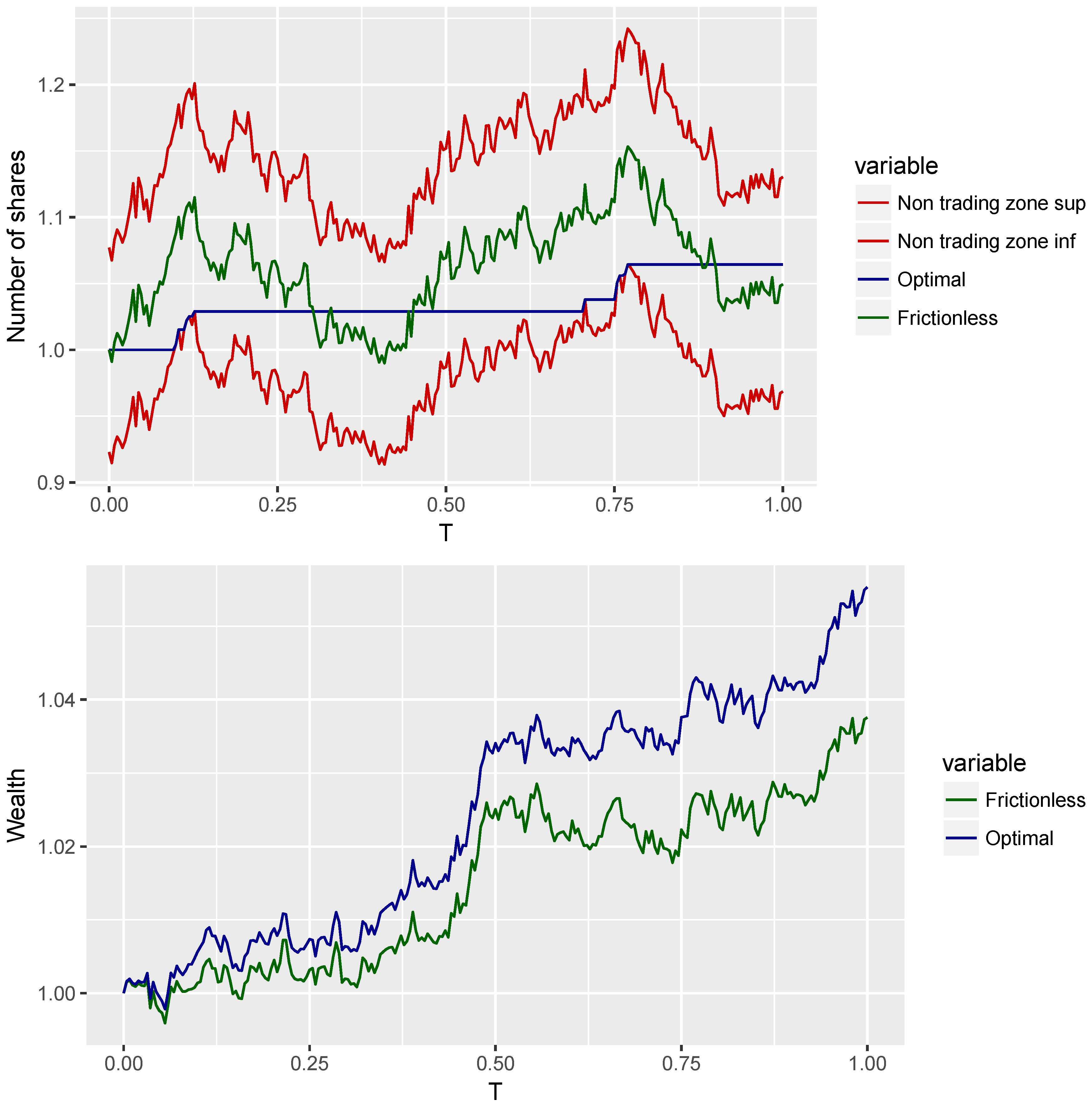
Recall that, by Lemma 2, the optimal policy in the frictionless case is to keep the ratio between the number of fund shares, s t , and the quotient W t e r ( T t ) W ̲ R t of the benchmark-adjusted wealth process, W t e r ( T t ) W ̲ , to the fund value, R t , at a constant level s * given by the risk-return tradeoff of the fund, α r σ 2 , normalized by the risk aversion γ . Proposition 1 shows that in the presence of transaction costs, the optimal policy is to keep the number of shares within a band around the quotient W t e r ( T t ) W ̲ R t . The width of this band is increasing in the transaction costs size ε : the larger the cost, the costlier it is to track the optimal position s t because the latter is too volatile and moves too much with W t and R t . Figure 1 illustrates the inefficiency of frequent rebalancing: while following s t of Lemma 2 would be optimal absent costs, in the presence of costs, it leads to significant losses, and the returns from following the strategy of Proposition 1 significantly dominate the returns from following the frictionless strategy, despite infrequent rebalancing.
Our explicit expression for the width parameter of the no-trading zone, C * , allows us to derive several interesting comparative statics results. The following result follows directly from the expression:
Proposition 2.
The following is true:
  • If α > r + γ σ 2 , then C * is monotone increasing in α and monotone decreasing in σ;
  • if α > r + γ σ 2 and γ 1 μ / σ F > β σ F , then C * is monotone decreasing in γ ;
  • If γ 1 μ / σ F > β σ F , then C * is monotone decreasing in both β and σ F ;
  • C * is monotone decreasing in μ for μ ( , β σ F 2 γ ) , and is monotone increasing in μ otherwise.
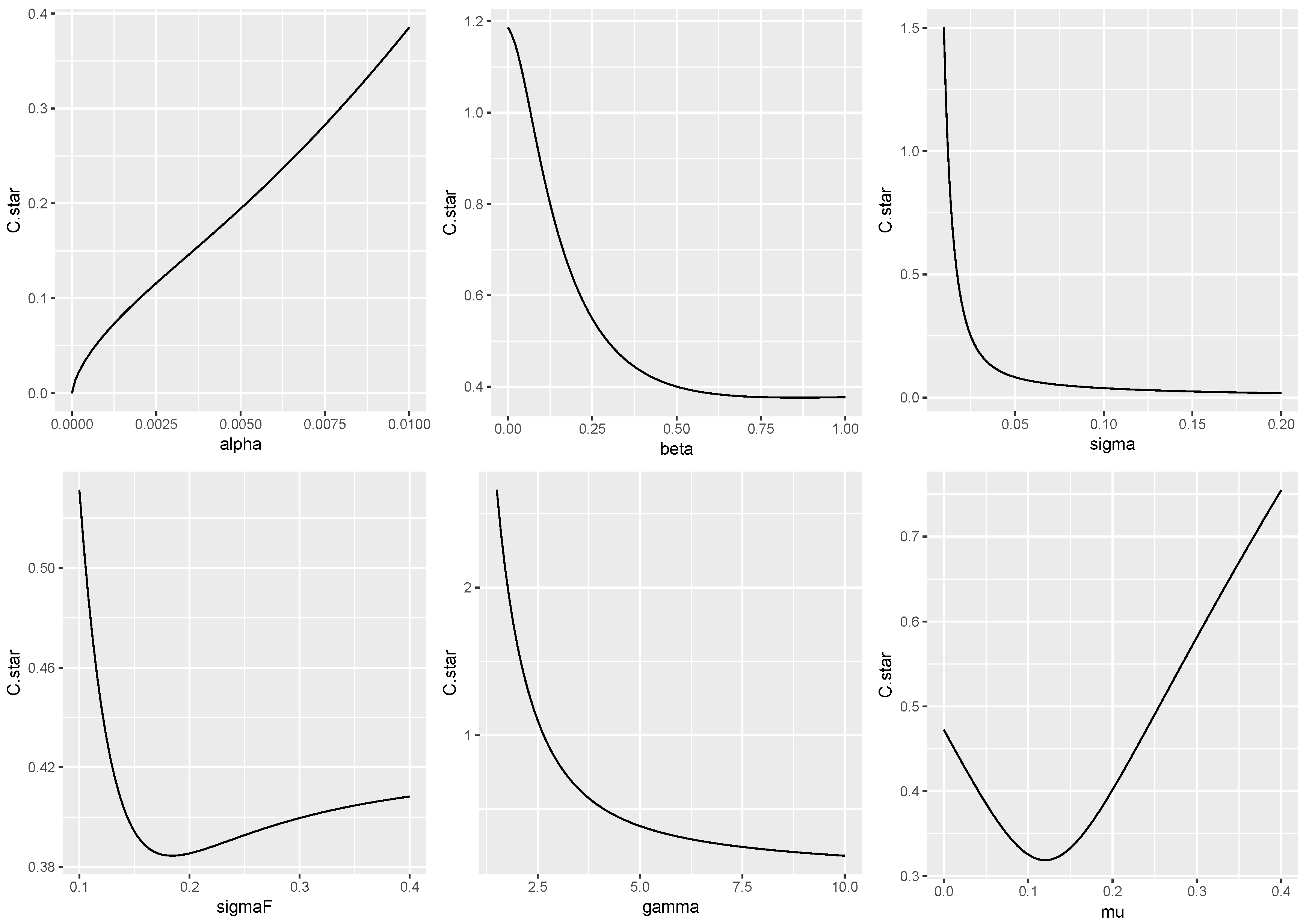
Proposition 2 and Figure 2 show that C * may exhibit complex behavior. First, C * tends to be monotone increasing in α : when the asset is good (with α large relative to risk, σ ), it is less expensive to hedge and stay exposed to α than to rebalance. Second, when risk aversion is higher, the agent finds it optimal to track the target portfolio as close as possible because the utility cost of an inefficient amount of risk taking is high; hence, C * tends to be decreasing in γ . The effect of unhedgeable risk is similar: a larger σ increases the utility cost of inefficient portfolio and hence triggers a more frequent rebalancing, implying that C * is decreasing in σ . The effects of σ F and μ (the parameters of the futures price process) are more subtle. For small values of σ F and μ , the risk-return tradeoff effect of the illiquid asset dominates: a larger μ or a larger σ F makes it more costly to deviate from the target. However, when μ is large, the ratio α / μ is small, and hence, the liquid futures contract becomes a good substitute for the illiquid asset. Thus, it becomes less important to hold the efficient exposure to the illiquid asset, and the no-trade band widens.

The Response of the No-Trading Zone to Shocks

The following proposition follows by direct calculation.
Proposition 3.
Inside the no-trade region, the wealth dynamics is given by:
W t = Ξ t ( W 0 + 0 t r + s R τ ( α + β μ r ) y * e r ( T τ ) W ̲ μ s R τ β σ F y * σ F Ξ τ d τ + 0 t s R τ β σ F Ξ τ d Z τ + 0 t s R τ σ Ξ τ d B τ )
with:
Ξ t e ( y * μ 0 . 5 ( y * σ F ) 2 ) t + y * σ F Z t ,
where s is the number of shares of the illiquid asset.
Proof. 
See Appendix A. ☐
Because the number of shares does not change inside the no-trading zone, the frictional wealth process W t deviates from its frictionless counterpart in Lemma 2. In particular, while the hedging ratio, y t / ( s t R t ) is constant in the frictionless case, it exhibits a non-trivial behavior in the presence of frictions. The following is a direct consequence of Proposition 3 and Lemma 2:
Corollary 1.
Inside the no-trading zone, given the illiquid asset position, s , the hedging ratio satisfies:
d y t s R t = μ t y d t + y * 1 W t e r ( T t ) W ̲ s R t R t 1 d R t + ( y * ) 2 W t e r ( T t ) W ̲ s R t F t 1 d F t .
Thus, the sensitivity of the hedging ratio to shocks d R t is positive if and only if s R t > ( W t e r ( T t ) W ̲ ) . That is, when R t is high relative to W t , a negative shock to R t leads to a drop in the hedging ratio. By contrast, when R t is low, hedging substitutes for rebalancing: a negative shock to R t leads to a drop in the hedging ratio. Furthermore, the sensitivity of the hedging ratio to shocks d F t is always positive.
Proof. 
See Appendix A. ☐
The intuition behind this result is straightforward: the response of y t to d R t depends on the contribution of R t to total wealth (net of benchmark), W t e r ( T t ) W ̲ . When this contribution is large, its contribution to the numerator in y t R t dominates, and the hedging ratio responds positively to shocks to R t . By contrast, when s R t is low, W t barely responds to shocks to R t , and hence, the denominator in y t R t dominates, making the hedging ratio respond negatively to shocks to R t .
By Proposition 1, the width 2 Δ t of the no-trading zone is proportional to y t / s R t . Thus, all results of Corollary 1 translate directly into analogous results for the no-trading zone.
Corollary 2.
Inside the no-trading zone, given the illiquid asset position, s , the sensitivity of Δ t to shocks d R t is positive if and only if s R t > ( W t e r ( T t ) W ̲ ) . That is, when R t is high relative to W t , a negative shock to R t narrows the no-trading zone. By contrast, when R t is low, a negative shock to R t leads to a widening of the no-trading zone. Furthermore, the sensitivity of the hedging ratio to shocks d F t is always positive.
Proof. 
See Appendix A. ☐
The intuition behind this result is similar to that for Corollary 1: when s R t is large relative to W t e r ( T t ) W ̲ , it is less expensive for the agent to hedge rather then to sell. By contrast, when s R t is small, the illiquid asset’s contribution is already so small that it is more efficient for the agent to sell.
Author Contributions

Conceptualization: F.G. and S.K.; validation: F.G. and S.M., formal analysis: F.G., S.K., and S.M.; original draft preparation: F.G., S.K., and S.M.

Funding

This research received no external funding.

Conflicts of Interest

The authors report no conflicts of interest. The authors alone are responsible for the content and writing of the paper.

Appendix A. Proofs

Proof of Lemma 1.
We have:
log ( R t / R 0 ) = ( α + β μ 0 . 5 ( β 2 σ F 2 + σ 2 ) ) t + β σ F Z t + σ B t log ( F t / F 0 ) = ( μ 0 . 5 σ F 2 ) t + σ F Z t .
Thus,
Z t B t = 0 σ F 1 σ 1 β σ log ( R t / R 0 ) ( α + β μ 0 . 5 ( β 2 σ F 2 + σ 2 ) ) t log ( F t / F 0 ) ( μ 0 . 5 σ F 2 ) t = σ F 1 ( log ( F t / F 0 ) ( μ 0 . 5 σ F 2 ) t ) σ 1 ( log ( R t / R 0 ) ( α + β μ 0 . 5 ( β 2 σ F 2 + σ 2 ) ) t ) β σ ( log ( F t / F 0 ) ( μ 0 . 5 σ F 2 ) t ) = σ F 1 ( log ( F t / F 0 ) ( μ 0 . 5 σ F 2 ) t ) σ 1 log ( R t / R 0 ) β σ log ( F t / F 0 ) σ 1 ( α 0 . 5 ( ( β 2 β ) σ F 2 + σ 2 ) ) t
and therefore:
M t = e r t λ 1 Z t λ 2 B t 0 . 5 t ( λ 1 2 + λ 2 2 ) = e r t μ σ F σ F 1 ( log ( F t / F 0 ) ( μ 0 . 5 σ F 2 ) t ) α r σ σ 1 log ( R t / R 0 ) β σ log ( F t / F 0 ) σ 1 ( α 0 . 5 ( ( β 2 β ) σ F 2 + σ 2 ) ) t 0 . 5 t ( λ 1 2 + λ 2 2 ) = exp α r σ 2 log ( R t / R 0 ) μ σ F 2 ( α r ) β σ 2 log ( F t / F 0 ) t Υ
where we have defined:
Υ r + 0 . 5 ( λ 1 2 + λ 2 2 ) μ σ F ( μ 0 . 5 σ F 2 ) α r σ 2 ( α 0 . 5 ( ( β 2 β ) σ F 2 + σ 2 ) )
 ☐
Proof of Lemma 2.
Since markets are dynamically complete, standard duality results imply that the optimal wealth profile is given by the solution to (3). By direct calculation, this solution is given by:
W T * = W ̲ + ν M T 1 / γ
where ν is determined by:
ν = W 0 e r T W ̲ E [ M T 1 γ 1 ] .
Thus, it remains to find the unique replicating portfolio.
By the Girsanov theorem,
Z T Q B T Q = λ T + Z T B T
is a Brownian motion under the risk neutral measure, so that:
M T = e r T λ 1 Z T λ 2 B T 0 . 5 T ( λ 1 2 + λ 2 2 ) = e r T λ 1 ( Z T Q T λ 1 ) λ 2 ( B T Q T λ 2 ) 0 . 5 T ( λ 1 2 + λ 2 2 ) = A T e λ 1 Z T Q λ 2 B T Q ,
where we have defined:
A T = e r T + 0 . 5 T ( λ 1 2 + λ 2 2 ) .
We have:
X ( t , ζ t ) = E t Q [ M T 1 / γ ] = E t Q [ A T 1 / γ e γ 1 ( λ 1 Z T Q + λ 2 B T Q ) ] = A T 1 / γ e γ 1 ζ t E t Q [ e γ 1 ( λ 1 ( Z T Q Z t Q ) + λ 2 ( B T Q B t Q ) ) ] = b e γ 1 ζ t ,
where we have defined:
b = A T 1 / γ e 0 . 5 ( ( γ 1 λ 1 ) 2 + γ 2 λ 2 2 ) ( T t )
and:
ζ t ( λ 1 Z t Q + λ 2 B t Q ) .
Thus,
X ( t , ζ t ) = ( e r T + 0 . 5 T ( λ 1 2 + λ 2 2 ) ) 1 / γ e 0 . 5 ( ( γ 1 λ 1 ) 2 + γ 2 λ 2 2 ) ( T t ) e γ 1 ζ t = ( e ( r + 0 . 5 ( λ 1 2 + λ 2 2 ) ) T ) 1 / γ e 0 . 5 ( ( γ 1 λ 1 ) 2 + γ 2 λ 2 2 ) ( T t ) A t γ 1 M t γ 1 = M t γ 1 e ( r + 0 . 5 ( λ 1 2 + λ 2 2 ) ) ( T t ) γ 1 e 0 . 5 ( ( γ 1 λ 1 ) 2 + γ 2 λ 2 2 ) ( T t ) = M t γ 1 e r ( T t ) γ 1 + 0 . 5 ( λ 1 2 + λ 2 2 ) ( γ 2 γ 1 ) ( T t )
Then, we have:
W t = E t [ ( M T / M t ) W T ] = e r ( T t ) W ̲ + ν M t 1 E t [ M T 1 γ 1 ] = e r ( T t ) ( W ̲ + ν E t Q [ M T 1 / γ ] ) .
Furthermore,
W T = e r T W 0 + 0 T e r ( T t ) ( x t ( R t 1 d R t r d t ) + y t F t 1 d F t ) = e r T W 0 + 0 T e r ( T t ) ( x t ( ( α + β μ ) d t + β σ F d Z t + σ d B t r d t ) + y t ( μ d t + σ F d Z t ) ) = e r T W 0 + 0 T e r ( T t ) ( x t ( β σ F d Z t Q + σ d B t Q ) + y t σ F d Z t Q ) = e r T W 0 + 0 T ( x ^ t d Z t Q + y ^ t d B t Q ) ,
where we have defined:
x ^ t = e r ( T t ) ( β σ F x t + y t σ F ) , y ^ t = e r ( T t ) x t σ .
Define:
F ( Z , B ) ν A 1 / γ e γ 1 ( λ 1 Z + λ 2 B ) + W ̲ ,
Then,
W T = ν M T 1 / γ + W ̲ = F ( Z T Q , B T Q )
By the Clark–Ocone formula, (A7) implies that:
x ^ t = E t Q [ F Z ( Z T Q , B T Q ) ] , y ^ t = E t Q [ F B ( Z T Q , B T Q ) ]
and then, you recover x t , y t from:
e r ( T t ) x ^ t = β σ F x t + y t σ F , e r ( T t ) y ^ t = x t σ ,
so that:
x t = e r ( T t ) σ 1 y ^ t , y t = e r ( T t ) σ F 1 ( x ^ t β σ F x t ) = e r ( T t ) ( σ F 1 x ^ t β σ 1 y ^ t ) .
By direct calculation, we have:
F Z ( Z T Q , B T Q ) = γ 1 λ 1 ν A 1 / γ e γ 1 ( λ 1 Z + λ 2 B )
and:
F B ( Z T Q , B T Q ) = γ 1 λ 2 ν A 1 / γ e γ 1 ( λ 1 Z + λ 2 B )
and hence:
x ^ t = γ 1 λ 1 ν X ( t , ζ t ) , y ^ t = γ 1 λ 2 ν X ( t , ζ t ) ,
and therefore:
x t = e r ( T t ) σ 2 γ 1 ( α r ) ν X ( t , ζ t ) , y t = e r ( T t ) ( σ F 1 ( γ 1 μ σ F 1 ) β σ 2 γ 1 ( α r ) ) ν X ( t , ζ t )
 ☐
Proof of Proposition 1.
We first compute the effective risk aversion. We have:
U ( t , W t , ζ t ) = E t [ ( W T W ̲ ) 1 γ ] = E t [ ν t 1 γ M T 1 1 / γ ] ,
where:
ν t = W t e r ( T t ) W ̲ E t [ M T 1 γ 1 ] ,
and hence:
Γ t = U w U w w = 1 γ ( W t e r ( T t ) W ̲ ) .
Then, we have:
d s t = d ( x t / R t ) = d t + R t 1 d x t R t 2 x t d R t = d t + R t 1 ν e r ( T t ) α r σ 2 γ 1 X ( t , ζ t ) ( γ 1 ( λ 1 d Z t Q + λ 2 d B t Q ) ) R t 1 x t ( β σ F d Z t Q + σ d B t Q ) ,
and hence, the quadratic variation of the number of shares in the fund is given by:
χ t d s t d t = R t 2 x t 2 γ 1 μ / σ F β σ F 2 + γ 1 ( α r ) / σ σ 2 .
The claim now follows from the general result in Kallsen and Muhle-Karbe (2017). ☐
Proof of Proposition 3.
We have:
d W t = r W t d t + s ( d R t r R t d t ) + y * ( W t e r ( T t ) W ̲ ) F t 1 d F t = r W t d t + s R t ( α + β μ r ) d t + s R t ( β σ F d Z t + σ d B t ) + y * ( W t e r ( T t ) W ̲ ) ( μ d t + σ F d Z t ) = ( r + y * μ ) W t d t + ( s R t ( α + β μ r ) y * e r ( T t ) W ̲ μ ) d t + ( s R t β σ F + y * W t σ F ) d Z t + s R t σ d B t .
Define:
Ξ t e ( y * μ 0 . 5 ( y * σ F ) 2 ) t + y * σ F Z t .
Then,
W τ = Ξ τ ( W 0 + 0 τ r + s R t ( α + β μ r ) y * e r ( T t ) W ̲ μ s R t β σ F y * σ F Ξ t d t + 0 τ s R t β σ F Ξ t d Z t + 0 τ s R t σ Ξ t d B t )
Proof of Corollary 1.
The dynamics of the hedging ratio is given by:
s d ( y t / ( s R t ) ) = R t 1 d y t R t 2 y t d R t + 0 . 5 2 R t 2 d R t , y t + 2 y t R t 3 d R t = R t 1 y * d W t R t 2 y t d R t + 0 . 5 2 R t 2 d R t , y t + 2 y t R t 3 d R t = R t 1 y * ( r W t d t + s ( d R t r R t d t ) + y * ( W t e r ( T t ) W ̲ ) F t 1 d F t ) R t 2 y * ( W t e r ( T t ) W ̲ ) d R t + 0 . 5 2 R t 2 d R t , y t + 2 y t R t 3 d R t .
The claim follows. ☐

References

  1. Almgren, Robert F. 2003. Optimal execution with nonlinear impact functions and trading-enhanced risk. Applied Mathematical Finance 10: 1–18. [Google Scholar] [CrossRef] [Green Version]
  2. Bichuch, Maxim. 2011. Asymptotic analysis for optimal investment in finite time with transaction costs. SIAM Journal of Financial Mathematics 3: 433–58. [Google Scholar] [CrossRef]
  3. Bichuch, Maxim, and Paolo Guasoni. 2018. Investing with Liquid and Illiquid Assets. Mathematical Finance 28: 119–52. [Google Scholar] [CrossRef]
  4. Bichuch, Maxim, and Steven Shreve. 2013. Utility Maximization Trading Two Futures with Transaction Costs. SIAM Journal of Financial Mathematics 4: 26–85. [Google Scholar] [CrossRef] [Green Version]
  5. Choi, Jin Hyuk. 2018. Optimal investment and consumption with liquid and illiquid assets. arXiv, arXiv:1602.06998. [Google Scholar]
  6. Collin-Dufresne, Pierre, Kent Daniel, Ciamac C. Moallemi, and Mehmet Saglam. 2012. Strategic Asset Allocation with Predictable Returns and Transaction Costs. Working Paper. Available online: https://www.risk.net/asset-management/insurance/2360849/optimal-trading-under-proportional-transaction-costs (accessed on 14 September 2018).
  7. Constantinides, George M. 1986. Capital market equilibrium with transaction costs. Journal of Political Economy 94: 842–62. [Google Scholar] [CrossRef]
  8. Cvitanic, Jaksa, and Ioannis Karatzas. 1996. Hedging and portfolio optimization under transaction costs: A martingale approach. Mathematical Finance 6: 133–65. [Google Scholar] [CrossRef]
  9. Dai, Min, Hanqing Jin, and Hong Liu. 2011. Illiquidity, position limits, and optimal investment for mutual funds. Journal of Economic Theory 146: 1598–630. [Google Scholar] [CrossRef]
  10. Dai, Min, Zuoquan Xu, and Xunyu Zhou. 2010. Continuous-time Markowitz model with transaction costs. SIAM Journal of Financial Mathematical 1: 96–125. [Google Scholar] [CrossRef]
  11. Davis, Mark H. A., and Andrew R. Norman. 1990. Portfolio selection with transaction costs. Mathematics of Operations Research 15: 676–713. [Google Scholar] [CrossRef]
  12. De Lataillade, Joachim, Cyril Deremble, Marc Potters, and Jean-Philippe Bouchaud. 2012. Optimal trading with linear costs. Journal of Investment Strategies 1: 91–115. [Google Scholar] [CrossRef] [Green Version]
  13. Dumas, Bernard, and Elisa Luciano. 1991. An exact solution to a dynamic portfolio choice problem under transaction costs. Journal of Finance 46: 577–95. [Google Scholar] [CrossRef]
  14. Dumas, Bernard, Francisco Delgado, and Giovanni W. Puopolo. 2015. Hysteresis bands on returns, holding period and transaction costs. Journal of Banking and Finance 57: 86–100. [Google Scholar]
  15. Garleanu, Nicolae, and Lasse Heje Pedersen. 2013. Dynamic trading with predictable returns and transaction costs. Journal of Finance 68: 2309–40. [Google Scholar] [CrossRef]
  16. Hobson, David, Alex S. L. Tse, and Yeqi Zhu. 2016. Optimal consumption and investment under transaction costs. arXiv, arXiv:1612.00720. [Google Scholar]
  17. Janecek, Karel, and Steven E. Shreve. 2004. Asymptotic analysis for optimal investment and consumption with transaction costs. Finance and Stochastics 8: 181–206. [Google Scholar] [CrossRef] [Green Version]
  18. Janecek, Karel, and Steven E. Shreve. 2010. Futures trading with transaction costs. Illinois Journal of Mathematics 54: 1239–84. [Google Scholar]
  19. Kallsen, Jan, and Johannes Muhle-Karbe. 2015. Option pricing and hedging with small transaction costs. Mathematical Finance 25: 702–23. [Google Scholar] [CrossRef]
  20. Kallsen, Jan, and Johannes Muhle-Karbe. 2017. The General Structure of Optimal Investment and Consumption with Small Transaction Costs. Mathematical Finance 27: 659–703. [Google Scholar] [CrossRef]
  21. Liu, Hong. 2005. Optimal Consumption and Investment with Transaction Costs and Multiple Risky Assets. Journal of Finance 59: 289–338. [Google Scholar] [CrossRef]
  22. Markowitz, Harry. 1952. Portfolio Selection. Journal of Finance 7: 77–91. [Google Scholar]
  23. Martin, Richard. 2014. Optimal trading under proportional transaction costs. Risk 27: 54–59. [Google Scholar]
  24. Martin, Richard, and Torsten Schöneborn. 2011. Mean reversion pays, but costs. Risk 24: 84–89. [Google Scholar]
  25. Merton, Robert C. 1969. Lifetime portfolio selection under uncertainty: The continuous-time case. Review of Economics and Statistics 51: 247–57. [Google Scholar] [CrossRef]
  26. Merton, Robert C. 1971. Optimum consumption and portfolio rules in a continuous-time model. Journal of Economic Theory 3: 373–413. [Google Scholar] [CrossRef] [Green Version]
  27. Shreve, Steven E., and Halil Mete Soner. 1994. Optimal investment and consumption with transaction costs. Annals of Applied Probability 4: 609–92. [Google Scholar] [CrossRef]
  28. Whalley, Elisabeth, and Paul Wilmott. 1997. An asymptotic analysis of an optimal hedging model for option pricing with transaction costs. Mathematical Finance 7: 307–24. [Google Scholar] [CrossRef]
1
For processes with infinite total variation, losses from transaction costs are infinite.
Figure 1. Simulated discrete time approximation of the P&L of the two strategies (the frictionless one, s t , from Lemma 2; and the optimal one, s ˜ t , of Proposition 1), net after transaction costs. Parameter values are: γ = 5 , c = 0 . 2 , μ = 0 . 05 , r = 0 , σ = 0 . 02 , σ F = 0 . 2 , α = 0 . 01 , β = 0 . 6 , ε = 0 . 01 , W 0 = 1 . Given the simulated paths of the two Brownian motions, the wealth curve reports the cumulative wealth of an agent following the respective strategy, net of costs. Since the frictionless strategy trades too frequently, losses due to costs are larger, and hence, the wealth of an agent following the frictionless strategy is lower than the wealth of an agent following the optimal strategy that account for costs.
Risks 06 00112 g001
Figure 2. The dependence of C * on the model parameters. In each plot, except for the varying parameter, all other parameters are fixed at their values of γ = 5 , c = 0 . 2 , μ = 0 . 05 , r = 0 , σ = 0 . 02 , σ F = 0 . 2 , α = 0 . 01 , β = 0 . 6 , ε = 0 . 01 , W 0 = 1 .
Risks 06 00112 g002