The Stability of the Aggregate Loss Distribution

Abstract

In this article we introduce the stability analysis of a compound sum: it consists of computing the standardized variation of the survival function of the sum resulting from an infinitesimal perturbation of the common distribution of the summands. Stability analysis is complementary to the classical sensitivity analysis, which consists of computing the derivative of an important indicator of the model, with respect to a model parameter. We obtain a computational formula for this stability from the saddlepoint approximation. We apply the formula to the compound Poisson insurer loss with gamma individual claim amounts and to the compound geometric loss with Weibull individual claim amounts.

1. Introduction

This article presents a computational formula for the stability of the survival function (s.f.) of the compound sum of independent and identically distributed (i.i.d.) random variables that are independent of their summation index. The compound sum typically represents the insurer total claim amount during a fixed period (e.g., a year): the i.i.d. random variables are the individual claim amounts and the number of claims within the period is a counting random variable or a counting stochastic process, if we let the period length vary. We define the stability of a sum as the standardized variation of the s.f. of the sum resulting from an infinitesimal perturbation at some point $x\in \mathbb{R}$ of the distribution of the summands.

More precisely, let ${\Delta }_x$ denote the Dirac distribution function (d.f.) over $\mathbb{R}$ with mass one at x (thus jumping from level 0 to level 1 at point x). If F denotes the d.f. of the summands, then

$$\begin{array}{cc}\hfill F_{x\epsilon }& =(1-\epsilon )F+\epsilon {\Delta }_x\hfill \end{array}$$

(1)

is the $\epsilon$-perturbation of F at x, for any choice of $\epsilon \in [0,1]$. The derivative of the s.f. of the sum under $F_{x\epsilon }$ with respect to (w.r.t.) $\epsilon$ evaluated at $\epsilon =0$ is the s.f. stability (s.f.s.) at the perturbation point x.

This concept differs from the one of sensitivity of queueing theory or risk theory, which is defined as the derivative of the s.f. of the sum w.r.t. a parameter of F (cf., e.g., Asmussen and Albrecher (2010), sct. IV.9). From an abstract point of view, a parametric model spans only a low-dimensional or narrow subset of the space of probability distributions. Such a narrow subset is indeed beneficial to statistical data reduction, but often does not contain all realistic perturbations of the assumed model. In this sense, the sensitivity is a limited indicator of the model stability. Allowing for perturbations in all possible directions provides a more complete or realistic analysis of the model stability. In this sense, our concept of stability is preferable. This concept is in fact an important idea of robust statistics (e.g., Hampel et al. (1986)). Mathematically, the quantity of interest of a stochastic model is regarded as a functional, and a functional derivative is computed. This approach is used, for example, in renewal theory by Grübel (1989), where the renewal function is a functional of the lifetime distribution, or by Politis (2006) for the probability of ruin of the risk process.

Practically, for a given actuarial aggregate loss model in the form of a compound sum, if a stability of low magnitude results from the perturbation in the form of a new large individual claim amount (viz. a large value of x), then the loss model is reliable under perturbations through extreme large claims. In the context of uncertainty (where for example catastrophic events are not incorporated in the model), this notion of stability appears practically relevant. The s.f.s. informs the risk manager about the variation of the upper tail probability of the aggregate loss when an uncertain large claim amount is considered. Still from the practical point of view, the sensitivity as described above has the alternative role of identifying important model parameters—the most significant ones have large sensitivity value. However, this interpretation holds only when the model is actually the correct one (which is often not simple to establish). Of course, both sensitivity and stability analyses can be carried out simultaneously.

Field and Ronchetti (1985) considered this type of stability for the sample mean and called it a “tail area influence function”. Their applications concerned statistical testing. They computed the tail area influence function with the saddlepoint approximation of Daniels (1954). This article generalizes this approximation to the stability of the compound sum and suggests using this concept in risk management. The new formula is easy and fast to compute. Numerical illustrations for the total claim amount with gamma or Weibull individual claim amounts and Poisson or geometric number of claims are provided.

Most methods for computing sensitivities rely on Monte Carlo simulation (e.g., Asmussen and Rubinstein (1999) and Asmussen and Glynn (2007), sct. VII). One exception is Gatto and Peeters (2015), who proposes evaluating the sensitivity of the s.f. of the random sum w.r.t. the parameter of the summation index distribution (which is either Poisson or geometric) with the saddlepoint approximation. Gatto and Peeters (2015) shows numerically that the sensitivities obtained by the saddlepoint approximation and by simulation with importance sampling are very close, even though importance sampling is computationally intensive. The high accuracy of the saddlepoint approximation is well illustrated in the literature of statistics and applied probability; refer, for example, to Jensen (1995) or to Gatto and Mosimann (2012) in the context of risk theory.

This article proceeds as follows. Section 2 provides the approximations to s.f.s. based on the saddlepoint approximation. Section 2.1 considers the the deterministic sum and Section 2.2 the compound sum, viz. the insurer aggregate claim amount. Section 3 provides numerical illustrations. Section 3.1 considers the aggregate claim amount with Poisson-distributed number of claims and gamma-distributed individual claim amounts. In Section 3.2, the number of claims follows the geometric distribution and the individual claim amounts follow the Weibull distribution. Some related long derivatives are provided in the Appendix A.

2. Saddlepoint Approximation to the Stability

This section has two parts: in Section 2.1 an approximation to s.f.s. of the deterministic sum is derived. It corresponds to the formula of Field and Ronchetti (1985), although the derivation is different. Section 2.2 generalizes the formula to the compound sum, which is an essential quantity of risk theory.

2.1. The Sum

Let $X_1,\dots ,X_n$ be independent random variables with d.f. F, moment generating function (m.g.f.) M and cumulant generating function (c.g.f.) $K=\log M$. The Legendre–Fenchel transform (or convex conjugate or large deviations index) of the c.g.f. K and at point $t\in \mathbb{R}$ is given by

$$\begin{array}{cc}\hfill \widehat{K}\left(t\right)& =\underset{v\in \mathrm{dom}K}{sup}vt-K\left(v\right)\in {\mathbb{R}}_{+}\cup \{\infty \},\hfill \end{array}$$

(2)

where $\mathrm{dom}\phi =\{x\in \mathbb{R}\mid |\phi \left(x\right)|<\infty \}$ is the domain of definition of $\phi :\mathbb{R}\to \mathbb{R}$. The transform $\widehat{K}$ is clearly nonnegative. One can show that it is convex and that it attains its minimum at $\mu =\mathsf{E}\left[X_1\right]$, when the expectation exists. Assume that the supremum (2) is attained at $v_t\in \mathrm{int}\mathrm{dom}K$. This condition is satisfied without restrictions on t when F is light-tailed, in the sense of having exponentially decaying tails. Under this assumption, $v_t$ solves w.r.t. v the equation

$$K^{\prime }\left(v\right)=t,$$

(3)

and convexity indicates that it is the unique solution. It is called the saddlepoint at t and $\widehat{K}\left(t\right)=v_{t}t-K\left(v_t\right)$. Define the sample mean by ${\overline{X}}_n={\sum }_{j=1}^n{X}_j/n$ and the s.f. ${\overline{H}}_n\left(t\right)={\mathsf{P}}_F[{\overline{X}}_n\ge t]$. Chernoff’s large deviations theorem states that $\forall t\ge \mu$,

$$\begin{array}{c}\hfill \frac{1}{n}\log {\overline{H}}_n\left(t\right)=-\widehat{K}\left(t\right)+\mathrm{o}\left(1\right),\mathrm{as}n\to \infty .\end{array}$$

(4)

Although (4) is a large deviations approximation, the asymptotics are in the logarithmic scale of the probability.

This article is based on the saddlepoint approximation of Lugannani and Rice (1980), because it is known that it provides a very accurate approximation to the s.f. ${\overline{H}}_n\left(t\right)$. It has bounded relative error on the probability scale, instead of the logarithmic scale. From now on, we assume that F is absolutely continuous. Under this additional assumption, Lugannani and Rice’s approximation to ${\overline{H}}_n\left(t\right)$ at $t\ne \mu$ is given by

$${\overline{G}}_n\left(t\right)=1-\mathsf{\Phi }\left(n^{\frac{1}{2}}r\right)+n^{-\frac{1}{2}}\varphi \left(n^{\frac{1}{2}}r\right)\left(\frac{1}{s}-\frac{1}{r}\right),$$

(5)

where

$$s=v_t{\left\{K^{″}\left(v_t\right)\right\}}^{\frac{1}{2}},r=\mathrm{sgn}\left(v_t\right){\left\{2\widehat{K}\left(t\right)\right\}}^{\frac{1}{2}},$$

(6)

and $\varphi$ and $\mathsf{\Phi }$ are the standard normal density and d.f., respectively. The relative error of approximation (5) is $\mathrm{O}\left(n^{-1}\right)$, as $n\to \infty$. For comparison, (4) re-expressed in terms of the new variable r leads to the quite dissimilar approximation to ${\overline{H}}_n\left(t\right)$ given by $\sqrt{2\pi }\varphi \left(n^{1/2}r\right)$.

The s.f.s. of ${\overline{X}}_n$ at tail value t and perturbation point $x\in \mathbb{R}$ is given by the Gâteaux differential

$${\tau }_n(t;x,F)=\frac{\partial }{\partial \epsilon }{\mathsf{P}}_{x\epsilon }[{\overline{X}}_n\ge t]{|}_{\epsilon =0},$$

(7)

where ${\mathsf{P}}_{x\epsilon }$ is the probability measure obtained by the replacement of the summand d.f. F by its $\epsilon$-perturbation at x, that is $F_{x\epsilon }$ defined in (1), for some $\epsilon \in [0,1]$. The following result gives an approximation to the s.f.s. obtained from (5).

Theorem 1.

Under the previous assumptions, the s.f.s. of ${\overline{X}}_n$ given in (7), at $t\ne \mu$ and at perturbation point $x\in \mathbb{R}$, can be approximated by

$$\begin{array}{cc}\hfill {\tilde{\tau }}_n(t;x,F)& =-n^{\frac{1}{2}}\varphi \left(n^{\frac{1}{2}}r\right)\left\{\frac{r{\dot{r}}_x}{s}+\mathrm{O}\left(n^{-1}\right)\right\},\hfill \end{array}$$

(8)

where s and r are given by (6), $v_t$ is given by (3), and

$${\dot{r}}_x=\frac{1}{r}\left(1-\exp \left\{v_t(x-t)+\frac{r^2}{2}\right\}\right).$$

(9)

The remainder term in (8) is given by

$$\begin{array}{c}\hfill -n^{-1}\left(\frac{{\dot{r}}_x}{r^2}-\frac{{\dot{s}}_x}{s^2}\right),\end{array}$$

where

$$\begin{array}{cc}\hfill {\dot{s}}_x& =\frac{v_t}{2s}\exp \left\{v_t(x-t)+\frac{r^2}{2}\right\}\left\{(t-x)\left(2+\frac{v_t^3}{s^2}{K}^{‴}\left(v_t\right)\right)+v_t{(t-x)}^2-\frac{s^2}{v_t}\right\}.\hfill \end{array}$$

(10)

Proof. 

Let $x\in \mathbb{R}$ and $\epsilon \in [0,1]$. The approximate s.f.s. (8) is obtained by differentiating w.r.t. $\epsilon$ the Lugannani and Rice saddlepoint approximation (5) at $F_{x\epsilon }$ and by evaluating it at $\epsilon =0$.

Let $v\in \mathbb{R}$, denote $M_{x\epsilon }\left(v\right)={\int }_{\mathbb{R}}{\mathrm{e}}^{vy}\mathrm{d}{F}_{x\epsilon }\left(y\right)$ and $K_{x\epsilon }=\log M_{x\epsilon }$. Then,

$$M_{x\epsilon }\left(v\right)=(1-\epsilon )M\left(v\right)+\epsilon {\mathrm{e}}^{vx}$$

(11)

(because for any Borel function $g:\mathbb{R}\to \mathbb{R}$, ${\int }_{\mathbb{R}}g\left(y\right)\mathrm{d}{\Delta }_x\left(y\right)=g\left(x\right)$). The perturbed saddlepoint $v_{tx\epsilon }$ at point $t\in \mathbb{R}$ is defined by $K_{x\epsilon }^{\prime }\left(v_{tx\epsilon }\right)=t$. Thus, from

$$K_{x\epsilon }^{\prime }\left(v_{tx\epsilon }\right)\sim K_{x\epsilon }^{\prime }\left(v_t\right)+(v_{tx\epsilon }-v_t)K_{x\epsilon }^{″}\left(v_t\right),\mathrm{as}\epsilon \to 0,$$

we obtain

$$\frac{v_{tx\epsilon }-v_t}{\epsilon }\sim \frac{t-K_{x\epsilon }^{\prime }\left(v_t\right)}{\epsilon K_{x\epsilon }^{″}\left(v_t\right)},\mathrm{as}\epsilon \to 0.$$

Consequently,

$${\dot{v}}_{tx}=\frac{\partial }{\partial \epsilon }{v}_{tx\epsilon }{|}_{\epsilon =0}=\underset{\epsilon \to 0}{lim}\frac{t-K_{x\epsilon }^{\prime }\left(v_t\right)}{\epsilon K_{x\epsilon }^{″}\left(v_t\right)}=\underset{\epsilon \to 0}{lim}\frac{-\frac{\partial }{\partial \epsilon }{K}_{x\epsilon }^{\prime }\left(v_t\right)}{K_{x\epsilon }^{″}\left(v_t\right)+\epsilon \frac{\partial }{\partial \epsilon }{K}_{x\epsilon }^{″}\left(v_t\right)}=-\frac{{\dot{K}}_x^{\prime }\left(v_t\right)}{K^{″}\left(v_t\right)},$$

(12)

where ${\dot{K}}_x^{\prime }\left(v\right)=\partial /\partial \epsilon$ $K_{x\epsilon }^{\prime }\left(v\right){\mid }_{\epsilon =0}$, see (A2) of the Appendix A. Thus, we obtain

$${\dot{v}}_{tx}=\frac{{\mathrm{e}}^{v_{t}x}(t-x)}{M\left(v_t\right)K^{″}\left(v_t\right)}.$$

Denote $r=r\left(F\right)$ in (6), then

$$\begin{array}{cc}\hfill {\dot{r}}_x& =\frac{\partial }{\partial \epsilon }r\left(F_{x\epsilon }\right){|}_{\epsilon =0}=\mathrm{sgn}\left(v_t\right)\frac{1}{2}{\left\{2[v_{t}t-K\left(v_t\right)]\right\}}^{-\frac{1}{2}}2\left[{\dot{v}}_{tx}t-\frac{\partial }{\partial \epsilon }{K}_{x\epsilon }\left(v_{tx\epsilon }\right){|}_{\epsilon =0}\right].\hfill \end{array}$$

(13)

Note that small perturbations do not affect the sign of $v_t$ when tail probabilities are considered. Precisely, if $t\ne \mathsf{E}\left[X_1\right]$, then $\mathrm{sgn}{v}_{tx\epsilon }=\mathrm{sgn}{v}_t$, $\forall \epsilon \in [0,{\epsilon }_0]$, for some ${\epsilon }_0>0$. Thus $\partial /\partial \epsilon \mathrm{sgn}{v}_{tx\epsilon }=0$, $\forall \epsilon \in [0,{\epsilon }_0]$. Define $g(\epsilon ,v)=K_{x\epsilon }\left(v\right)$, $g_1^{\prime }(\epsilon ,v)=\partial /\partial \epsilon g(\epsilon ,v)$, and $g_2^{\prime }(\epsilon ,v)=\partial /\partial vg(\epsilon ,v)$. Then, from the multivariate chain rule,

$$\frac{\partial }{\partial \epsilon }{K}_{x\epsilon }\left(v_{tx\epsilon }\right)=\frac{\partial }{\partial \epsilon }g(\epsilon ,v_{tx\epsilon })=g_1^{\prime }(\epsilon ,v_{tx\epsilon })+g_2^{\prime }(\epsilon ,v_{tx\epsilon })\frac{\partial }{\partial \epsilon }{v}_{tx\epsilon }=\left(\frac{\partial }{\partial \epsilon }{K}_{x\epsilon }\right)\left(v_{tx\epsilon }\right)+K_{x\epsilon }^{\prime }\left(v_{tx\epsilon }\right)\frac{\partial }{\partial \epsilon }{v}_{tx\epsilon }.$$

Hence, we obtain

$$\frac{\partial }{\partial \epsilon }{K}_{x\epsilon }\left(v_{tx\epsilon }\right){|}_{\epsilon =0}={\dot{K}}_x\left(v_t\right)+K^{\prime }\left(v_t\right){\dot{v}}_{tx},$$

where ${\dot{K}}_x\left(v\right)=\partial /\partial \epsilon$ $K_{x\epsilon }\left(v\right){\mid }_{\epsilon =0}$ (see (A1) in the Appendix A). By inserting this result into (13), we obtain (9).

Denote $s=s\left(F\right)$, then (6) leads to

$${\dot{s}}_x=\frac{\partial }{\partial \epsilon }s\left(F_{x\epsilon }\right){|}_{\epsilon =0}={\dot{v}}_{tx}{\left\{K^{″}\left(v_t\right)\right\}}^{\frac{1}{2}}+\frac{v_t}{2}{\left\{K^{″}\left(v_t\right)\right\}}^{-\frac{1}{2}}\frac{\partial }{\partial \epsilon }{K}_{x\epsilon }^{″}\left(v_{tx\epsilon }\right){|}_{\epsilon =0}.$$

From the multivariate chain rule, we obtain

$$\frac{\partial }{\partial \epsilon }{K}_{x\epsilon }^{″}\left(v_{tx\epsilon }\right){|}_{\epsilon =0}={\dot{K}}_x^{″}\left(v_t\right)+K^{‴}\left(v_t\right){\dot{v}}_{tx},$$

where ${\dot{K}}_x^{″}\left(v\right)=\partial /\partial \epsilon$ $K_{x\epsilon }^{″}\left(v\right){\mid }_{\epsilon =0}$ (see (A3) in the Appendix A). These two last results yield (10). ☐

The leading term of the approximation to the s.f.s. (8) is equal to Formula (3.1) in Field and Ronchetti (1985), which is however not derived from the saddlepoint approximation (5) but from the Laplace approximation to the integral of the saddlepoint approximation to the density of Daniels (1954). In order to control this equality, the following correspondences between the two notations can be useful: $C_F\left(t\right)=\exp \{\widehat{K}\left(t\right)\}$, ${\alpha }_F\left(t\right)=v_t$, ${\sigma }_F\left(t\right)={\left\{K^{″}\left(v_t\right)\right\}}^{1/2}$, and $\psi (x;t)=x-t$. Thus, Theorem 1 provides an alternative derivation of the s.f.s. of Field and Ronchetti (1985) as well as the exact form of the error term. However, numerical studies suggest that it is preferable to use the first-order term alone.

Regarding the sum, let $S_n={\sum }_{j=1}^n{X}_j$, then $\mathsf{P}[S_n\ge t]={\overline{H}}_n(t/n)$ is its s.f., its saddlepoint approximation is ${\overline{G}}_n(t/n)$, $\partial /\partial \epsilon {\mathsf{P}}_{x\epsilon }[S_n\ge t]{\mid }_{\epsilon =0}={\tau }_n(t/n;x,F)$ is its s.f.s., and the saddlepoint approximation is ${\tilde{\tau }}_n(t/n;x,F)$.

2.2. The Compound Sum

Let the random variables $X_1,X_2,\dots$ fulfill the assumptions given in Section 2.1 and let F denote their common d.f. Let N be an independent random variable taking values in $\{0,1,\dots \}$ with probability function $p_n=\mathsf{P}[N=n]$, for $n=0,1,\dots$ Consider the compound sum

$$\begin{array}{cc}\hfill Z& =\sum _{j=0}^N{X}_j,\hfill \end{array}$$

where $X_0=0$ by definition. Define the indicator $\mathrm{I}\left\{A\right\}$ as the function equal to 1 if the statement A is true, or equal to 0 if A is false. The s.f. of Z at $t\in \mathbb{R}$ can be written as

$$\begin{array}{cc}\hfill {\overline{H}}_Z\left(t\right)& ={\mathsf{P}}_F[Z\ge t]=p_0\mathrm{I}\{t\le 0\}+\sum _{n=1}^{\infty }{\int }_{{\mathbb{R}}^n}\mathrm{I}\left\{\sum _{k=1}^n{x}_k\ge t\right\}\prod _{k=1}^n\mathrm{d}F\left(x_k\right)p_n,\hfill \end{array}$$

(14)

which is generally not a computational formula. This section provides the saddlepoint approximation to (14), and then the associated approximation to the s.f.s.

In (14) we see that the distribution of Z is a linear combination of a distribution with mass one at zero and an absolutely continuous distribution. The mass at zero must be eliminated in order to apply the saddlepoint approximation. Denote by $M_N$ and $K_N$ the m.g.f. and the c.g.f. of N, respectively, and by K the c.g.f. of $X_1$. Then, the m.g.f of Z is $M_Z=M_N\circ K$, and its c.g.f. is $K_Z=K_N\circ K$. Let $Z_0$ be a random variable with the conditional distribution of Z given $N>0$. Then, ${\overline{H}}_{Z_0}\left(t\right)=\mathsf{P}[Z\ge t|N>0]$ and $K_{Z_0}\left(v\right)=\log \mathsf{E}\left[{\mathrm{e}}^{vZ}\right|N>0]$ are the s.f. and the c.g.f. of $Z_0$, respectively. The Legendre–Fenchel transform of the c.g.f. $K_{Z_0}$ at $t\in \mathbb{R}$ is given by

$$\begin{array}{cc}\hfill {\widehat{K}}_{Z_0}\left(t\right)& =\underset{v\in \mathrm{dom}{K}_{Z_0}}{sup}vt-K_{Z_0}\left(v\right).\hfill \end{array}$$

(15)

We assume that the supremum in (15) is attained at $v_t\in \mathrm{int}\mathrm{dom}{K}_{Z_0}$. Under this assumption, $v_t$ solves w.r.t. v the equation

$$\begin{array}{cc}\hfill K_{Z_0}^{\prime }\left(v\right)& =t.\hfill \end{array}$$

(16)

The solution $v_t$ is unique and called saddlepoint at t. We obtain the saddlepoint approximation to ${\overline{H}}_{Z_0}\left(t\right)$ at $t\ne \mathsf{E}\left[Z_0\right]$, denoted ${\overline{G}}_{Z_0}\left(t\right)$, by the left side of (5) with $n=1$ and with

$$s=v_t{\{K_{Z_0}^{″}\left(v_t\right)\}}^{\frac{1}{2}}\mathrm{and}r=\mathrm{sgn}\left(v_t\right){\{2{\widehat{K}}_{Z_0}\left(t\right)\}}^{\frac{1}{2}}.$$

(17)

It follows from

$$\begin{array}{cc}\hfill K_{Z_0}\left(v\right)& =\log \frac{M_Z\left(v\right)-p_0}{1-p_0}\hfill \end{array}$$

that (16) can be re-expressed as

$$\begin{array}{cc}\hfill \frac{M_N^{\prime }\left(K\left(v\right)\right)K^{\prime }\left(v\right)}{M_N\left(K\left(v\right)\right)-p_0}& =t.\hfill \end{array}$$

(18)

More explicit expressions of s and r than those in (17) are obtained with

$$\begin{array}{cc}\hfill K_{Z_0}^{″}\left(v_t\right)& =t\left(\frac{M_N^{″}\left(K\left(v_t\right)\right)K^{\prime }\left(v_t\right)}{M_N^{\prime }\left(K\left(v_t\right)\right)}+\frac{K^{″}\left(v_t\right)}{K^{\prime }\left(v_t\right)}-t\right)\hfill \end{array}$$

(19)

(see (A6) in the Appendix A), and by

$$r=\mathrm{sgn}\left(v_t\right){\left\{2[v_{t}t-\log \{M_N\left(K\left(v_t\right)\right)-p_0\}+\log \{1-p_0\}]\right\}}^{\frac{1}{2}}.$$

(20)

It follows from

$${\overline{H}}_Z\left(t\right)={\overline{H}}_{Z_0}\left(t\right)(1-p_0)+\mathrm{I}\{t\le 0\}{p}_0$$

(21)

that the saddlepoint approximation to ${\overline{H}}_Z\left(t\right)$ is given by

$${\overline{G}}_Z\left(t\right)={\overline{G}}_{Z_0}\left(t\right)(1-p_0)+\mathrm{I}\{t\le 0\}{p}_0.$$

(22)

The s.f.s. of Z is the Gâteaux differential

$${\tau }_Z(t;x,F)=\frac{\partial }{\partial \epsilon }{\mathsf{P}}_{x\epsilon }[Z\ge t]{|}_{\epsilon =0},$$

(23)

where $F_{x,\epsilon }$ is given by (1), $\forall x\in \mathbb{R}$, and $\epsilon \in [0,1]$. The following result gives an approximation to the s.f.s. ${\tau }_Z(t;x,F)$ obtained from the first-order approximation of the s.f.s. of the mean given in Theorem 1.

Theorem 2.

Under the previous assumptions, the s.f.s. given in (23) for the s.f. of Z at $t\ne \mathsf{E}\left[N\right]\mathsf{E}\left[X_1\right]/(1-p_0)$ and at perturbation $x\in \mathbb{R}$ can be approximated by

$${\tilde{\tau }}_Z(t;x,F)={\tilde{\tau }}_{Z_0}(t;x,F)(1-p_0),$$

(24)

where

$$\begin{array}{cc}\hfill {\tilde{\tau }}_{Z_0}(t;x,F)& =-\varphi \left(r\right)\frac{r{\dot{r}}_x}{s},\hfill \end{array}$$

s and r are given by (17), (19), and (20), $v_t$ is given in (18),

$${\dot{r}}_x=-\frac{{\dot{K}}_{Z_{0}x}\left(v_t\right)}{r},$$

(25)

and

$$\begin{array}{cc}\hfill {\dot{K}}_{Z_{0}x}\left(v_t\right)& =t\frac{\exp \{v_{t}x-K\left(v_t\right)\}-1}{K^{\prime }\left(v_t\right)}.\hfill \end{array}$$

(26)

Proof. 

This proof is similar to the one of Theorem 1, and so only the main arguments are given. Let $x\in \mathbb{R}$ and $\epsilon \in [0,1]$. Let us define the perturbed m.g.f. $M_{x\epsilon }$ as in (11), $K_{x\epsilon }=\log M_{x\epsilon }$, and for $v\in \mathbb{R}$,

$$K_{Z_{0}x\epsilon }\left(v\right)=\log \frac{M_N\left(K_{x\epsilon }\left(v\right)\right)-p_0}{1-p_0}.$$

By following the reasoning that led to (12) in the proof of Theorem 1, we obtain the perturbed saddlepoint at point $t\in \mathbb{R}$ as:

$${\dot{v}}_{tx}=-\frac{{\dot{K}}_{Z_{0}x}^{\prime }\left(v_t\right)}{K_{Z_0}^{″}\left(v_t\right)},$$

(27)

where ${\dot{K}}_{Z_{0}x}^{\prime }\left(v\right)=\partial /\partial \epsilon K_{Z_{0}x\epsilon }^{\prime }\left(v\right){\mid }_{\epsilon =0}$ is given by (A5) in the Appendix A. With (18), it simplifies to

$$\begin{array}{cc}\hfill {\dot{K}}_{Z_{0}x}^{\prime }\left(v_t\right)& =t\left(\frac{M_N^{″}\left(K\left(v_t\right)\right){\dot{K}}_x\left(v_t\right)}{M_N^{\prime }\left(K\left(v_t\right)\right)}+\frac{{\dot{K}}_x^{\prime }\left(v_t\right)}{K^{\prime }\left(v_t\right)}-\frac{{\dot{K}}_x\left(v_t\right)}{K^{\prime }\left(v_t\right)}t\right),\hfill \end{array}$$

(28)

where ${\dot{K}}_x\left(v\right)$ and ${\dot{K}}_x^{\prime }\left(v\right)$ are respectively given in (A1) and (A2) of the Appendix A.

By denoting $r=r\left(F\right)$, we find for $t\ne \mathsf{E}\left[Z_0\right]$,

$${\dot{r}}_x=\frac{\partial }{\partial \epsilon }r\left(F_{x\epsilon }\right){|}_{\epsilon =0}=\mathrm{sgn}\left(v_t\right)\frac{1}{2}{\left\{2[v_{t}t-K_{Z_0}\left(v_t\right)]\right\}}^{-\frac{1}{2}}2\left[{\dot{v}}_{tx}t-\frac{\partial }{\partial \epsilon }{K}_{Z_{0}x\epsilon }\left(v_{tx\epsilon }\right){|}_{\epsilon =0}\right].$$

The multivariate chain rule yields

$$\frac{\partial }{\partial \epsilon }{K}_{Z_{0}x\epsilon }\left(v_{tx\epsilon }\right){|}_{\epsilon =0}=K_{Z_0}^{\prime }\left(v_t\right){\dot{v}}_{tx}+{\dot{K}}_{Z_{0}x}\left(v_t\right),$$

where ${\dot{K}}_{Z_{0}x}=\partial /\partial \epsilon K_{Z_{0}x\epsilon }^{\prime }\left(v\right){\mid }_{\epsilon =0}$ is given in (A4) in the Appendix. By joining these two last expressions, one obtains (25) in the theorem. Then, (26) is obtained from (A4) and (A1) in the Appendix A, and from (18).

The s.f.s. of $Z_0$ is given by

$$\begin{array}{cc}\hfill {\tau }_{Z_0}(t;x,F)& =\frac{\partial }{\partial \epsilon }{\mathsf{P}}_{x\epsilon }[Z_0\ge t]{|}_{\epsilon =0}.\hfill \end{array}$$

Thus, it follows from (21) that

$$\begin{array}{cc}\hfill {\tau }_Z(t;x,F)& ={\tau }_{Z_0}(t;x,F)(1-p_0).\hfill \end{array}$$

This justifies (24) in the theorem. ☐

Remark 1.

Another approximation to the s.f.s. of Z can be obtained by generalizing the remainder term given in Theorem 1. This yields the approximation at $t\ne \mathsf{E}\left[Z_0\right]$ given by

$$\begin{array}{c}\hfill -\varphi \left(r\right)\left\{\frac{r{\dot{r}}_x}{s}-\left(\frac{{\dot{r}}_x}{r^2}-\frac{{\dot{s}}_x}{s^2}\right)\right\}(1-p_0),\end{array}$$

where

$${\dot{s}}_x=\frac{v_t}{s}\left\{-{\dot{K}}_{Z_{0}x}^{\prime }\left(v_t\right)\left(1+\frac{v_t}{2}\frac{K_{Z_0}^{‴}\left(v_t\right)}{K_{Z_0}^{″}\left(v_t\right)}\right)+\frac{v_t}{2}{\dot{K}}_{Z_{0}x}^{″}\left(v_t\right)\right\},$$

(29)

and with other quantities given in Theorem 2. The derivatives appearing in (29) are given by (28), (19),

$$\begin{array}{ccc}{K}_{Z_0}^{‴}\left(v_t\right)\hfill & =\hfill & t\left\{\frac{M_N^{‴}\left(K\left(v_t\right)\right){\left\{K^{\prime }\left(v_t\right)\right\}}^2+3M_N^{″}\left(K\left(v_t\right)\right)K^{″}\left(v_t\right)}{M_N^{\prime }\left(K\left(v_t\right)\right)}+\frac{K^{‴}\left(v_t\right)}{K^{\prime }\left(v_t\right)}\right.\hfill \\ & & \left.-3\left(\frac{M_N^{″}\left(K\left(v_t\right)\right)K^{\prime }\left(v_t\right)}{M_N^{\prime }\left(K\left(v_t\right)\right)}+\frac{K^{″}\left(v_t\right)}{K^{\prime }\left(v_t\right)}\right)t+2t^2\right\},\hfill \end{array}$$

(30)

and by

$$\begin{array}{cc}{\dot{K}}_{Z_{0}x}^{″}\left(v_t\right)\hfill & =t\left\{\frac{M_N^{‴}\left(K\left(v_t\right)\right){\dot{K}}_x\left(v_t\right)K^{\prime }\left(v_t\right)+2M_N^{″}\left(K\left(v_t\right)\right){\dot{K}}_x^{\prime }\left(v_t\right)}{M_N^{\prime }\left(K\left(v_t\right)\right)}+\frac{M_N^{″}\left(K\left(v_t\right)\right){\dot{K}}_x\left(v_t\right)K^{″}\left(v_t\right)}{M_N^{\prime }\left(K\left(v_t\right)\right)K^{\prime }\left(v_t\right)}\right.\hfill \\ & \left.+\frac{{\dot{K}}_x^{″}\left(v_t\right)}{K^{\prime }\left(v_t\right)}-\left(3\frac{M_N^{″}\left(K\left(v_t\right)\right){\dot{K}}_x\left(v_t\right)}{M_N^{\prime }\left(K\left(v_t\right)\right)}+2\frac{{\dot{K}}_x^{\prime }\left(v_t\right)}{K^{\prime }\left(v_t\right)}+\frac{K^{″}\left(v_t\right){\dot{K}}_x\left(v_t\right)}{{\left\{K^{\prime }\left(v_t\right)\right\}}^2}\right)t+2\frac{{\dot{K}}_x\left(v_t\right)}{K^{\prime }\left(v_t\right)}{t}^2\right\}.\hfill \end{array}$$

(31)

${\dot{K}}_x\left(v_t\right)$, ${\dot{K}}_x^{\prime }\left(v_t\right)$, and ${\dot{K}}_x^{″}\left(v_t\right)$ in (31) can be found respectively in (A1), (A2), and (A3) in the Appendix A.

The justification follows the proof of Theorem 1. By denoting $s=s\left(F\right)$, we have

$${\dot{s}}_x=\frac{\partial }{\partial \epsilon }s\left(F_{x\epsilon }\right){|}_{\epsilon =0}={\dot{v}}_{tx}{\left\{K_{Z_0}^{″}\left(v_t\right)\right\}}^{\frac{1}{2}}+\frac{v_t}{2}{\left\{K_{Z_0}^{″}\left(v_t\right)\right\}}^{-\frac{1}{2}}\frac{\partial }{\partial \epsilon }{K}_{Z_{0}x\epsilon }^{″}\left(v_{tx\epsilon }\right){|}_{\epsilon =0}.$$

From the multivariate chain rule we obtain

$$\frac{\partial }{\partial \epsilon }{K}_{Z_{0}x\epsilon }^{″}\left(v_{tx\epsilon }\right){|}_{\epsilon =0}=K_{Z_0}^{‴}\left(v_t\right){\dot{v}}_{tx}+{\dot{K}}_{Z_{0}x}^{″}\left(v_t\right).$$

These two last expressions and (27) give (29). Then, (30) follows from (A8), (28) follows from (A5), and (31) follows from (A7).

3. Numerical Illustrations

This section provides numerical illustrations of the results of Section 2.2 for two important aggregate loss models: the Poisson number of occurrences with gamma individual claim amounts, in Section 3.1, and the geometric number of occurrences with Weibull individual claim amounts, in Section 3.2.

This numerical study was performed with Matlab (R2017b, The MathWorks, Natick, MA, USA), and the function fminsearch was used for computing the saddlepoint. Matlab’s programs used for these computations are available at http://www.stat.unibe.ch.

3.1. Poisson-Gamma Total Claim Amount

Assume that the total number of claims of an insurance company that occur during a fixed time horizon, denoted by N, is Poisson-distributed with parameter $\lambda >0$; viz. $p_n=\mathsf{P}[N=n]=e^{-\lambda }{\lambda }^n/n!$, for $n=0,1,\dots$. Let $v\in \mathbb{R}$. The m.g.f. of N and its derivatives are given by

$$\begin{array}{c}\hfill M_N\left(v\right)=\exp \left\{\lambda ({\mathrm{e}}^v-1)\right\},M_N^{\prime }\left(v\right)=\lambda {\mathrm{e}}^v\exp \left\{\lambda ({\mathrm{e}}^v-1)\right\}\mathrm{and}{M}_N^{″}\left(v\right)=\lambda {\mathrm{e}}^v(1+\lambda {\mathrm{e}}^v)\exp \left\{\lambda ({\mathrm{e}}^v-1)\right\}.\end{array}$$

Assume that the individual claim amounts or losses $X_1,X_2,\dots$ are gamma-distributed, with density $f\left(y\right)={\beta }^{\alpha }/\mathsf{\Gamma }\left(\alpha \right)y^{\alpha -1}{\mathrm{e}}^{-\beta y}$, $\forall y>0$, for some parameters $\alpha ,\beta >0$. Let $v<\beta$. The c.g.f. of $X_1$ and its derivatives are given by

$$\begin{array}{c}\hfill K\left(v\right)=\alpha \log \frac{\beta }{\beta -v},K^{\prime }\left(v\right)=\frac{\alpha }{\beta -v}\mathrm{and}{K}^{″}\left(v\right)=\frac{\alpha }{{(\beta -v)}^2}.\end{array}$$

The m.g.f. of the aggregate loss $Z={\sum }_{j=0}^N{X}_j$ is given by

$$\begin{array}{cc}\hfill M_Z\left(v\right)& =\exp \left\{\lambda \left[{\left(\frac{\beta }{\beta -v}\right)}^{\alpha }-1\right]\right\},\hfill \end{array}$$

and so the c.g.f. of $Z_0$, viz. Z given $N>0$, is given by

$$\begin{array}{cc}\hfill K_{Z_0}\left(v\right)& =\log \frac{\exp \left\{\lambda {\left(\frac{\beta }{\beta -v}\right)}^{\alpha }\right\}-1}{{\mathrm{e}}^{\lambda }-1}.\hfill \end{array}$$

With these formulae we can obtain the values of s, r, and ${\dot{r}}_x$ required in Theorem 2. So, we can compute the s.f.s. $\tilde{\tau }(t;x,F)$ given in (24).

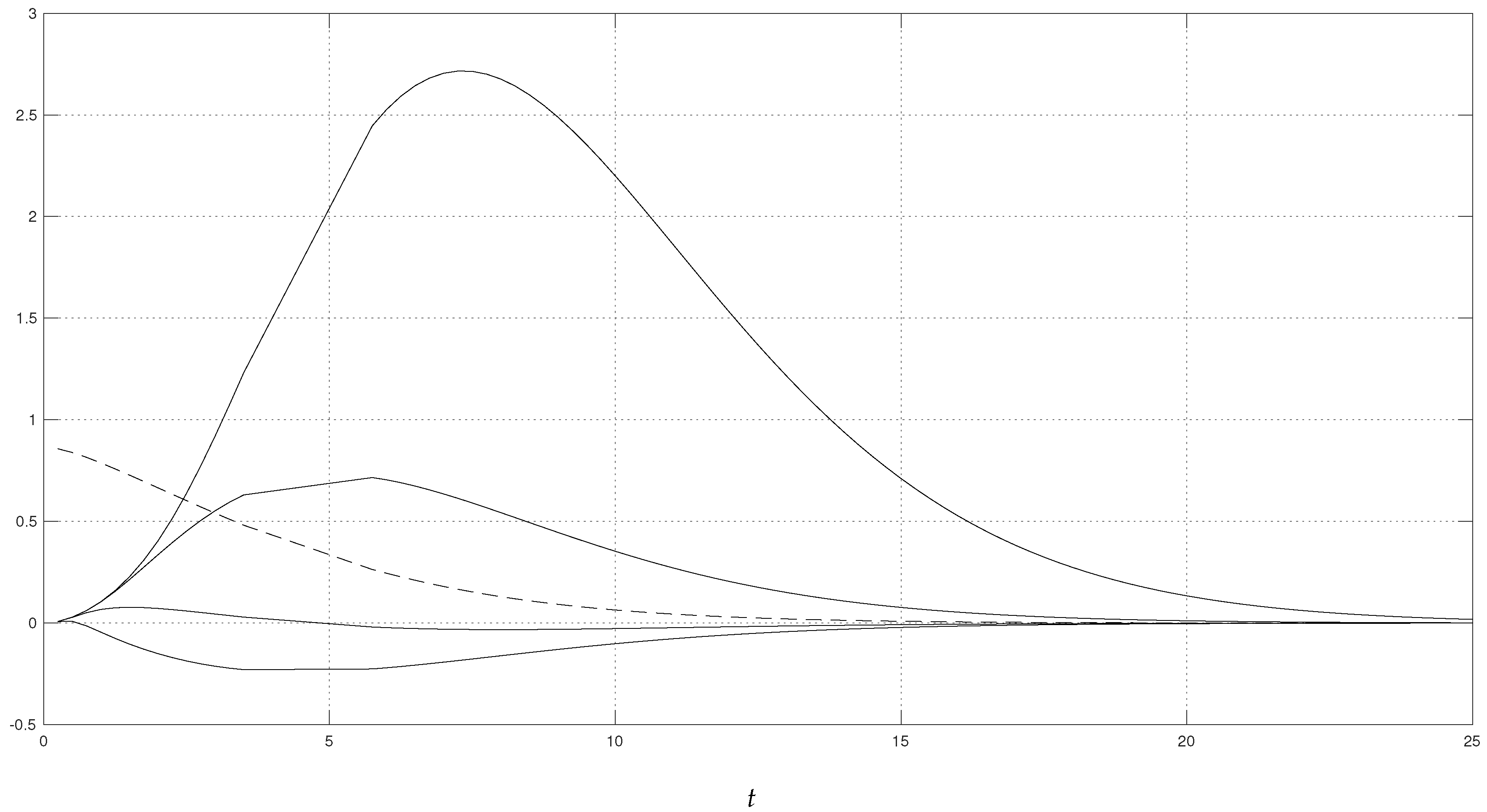
For the numerical illustration, we fixed $\lambda =2$, $\alpha =2$, and $\beta =3$. The results are shown in Figure 1. The dashed curve shows the saddlepoint approximation ${\overline{G}}_Z\left(t\right)$ to the s.f. (see (22)) for all relevant values of t. The four solid curves of Figure 1 show the approximation to the stability ${\tilde{\tau }}_Z(t;x,F)$, for the perturbation points $x=1,2,5,10$, and for relevant values of t. The highest curves correspond to the largest values of x. This is what we would have expected. A large perturbation point x yields a large increase of the upper tail probability, and thus a large value of the stability. A vanishing perturbation point x yields either a small increase or a decrease of the upper tail probability, and thus a small value of the stability. We should note that the numerical computation of these curves is very fast. Thus, the proposed approximation to the s.f.s. inherits the well-known computational efficiency of the saddlepoint approximation. Any purely numerical technique (e.g., Monte Carlo simulation) would be computationally intensive and thus slower.

Figure 1. Poisson with $\lambda =2$ compound sum of independent gamma with $\alpha =2$ and $\beta =3$ random variables. Dashed curve: s.f. Continuous curve, from lowest to highest curve: approximate stabilities for perturbation points $x=1,2,5,10$, respectively.

For a practical illustration, consider the following values from the setting of Figure 1: ${\overline{G}}_Z\left(14.75\right)=0.0099\simeq 1\%$ and ${\tilde{\tau }}_Z(14.75;10,F)=0.7639$. If the insurance believes that additional claim amounts of $x=10$ with small frequency $\epsilon =1$‰ have to be considered, then the tail probability of the non-perturbed model would rise by $7\%$, because $0.0099+0.001\times 0.7636=0.0107$.

3.2. Geometric-Weibull Total Claim Amount

The suggested approximation was tested with a different aggregate loss model. Assume that the total number of claims N follows the geometric distribution with parameter $\rho \in (0,1)$, precisely $p_n=\mathsf{P}[N=n]=\rho {(1-\rho )}^n$, for $n=0,1,\dots$. The m.g.f. of N and its derivatives at $v<-\log (1-\rho )$ are given by

$$\begin{array}{c}\hfill M_N\left(v\right)=\frac{\rho }{1-(1-\rho ){\mathrm{e}}^v},M_N^{\prime }\left(v\right)=\frac{\rho (1-\rho ){\mathrm{e}}^v}{{\left\{1-(1-\rho ){\mathrm{e}}^v\right\}}^2},\mathrm{and}{M}_N^{″}\left(v\right)=\frac{\rho \left(1-\rho \right){\mathrm{e}}^v\left\{1+\left(1-\rho \right){\mathrm{e}}^v\right\}}{{\left\{1-\left(1-\rho \right){\mathrm{e}}^v\right\}}^3}.\end{array}$$

Assume the individual losses $X_1,X_2,\dots$ follow the Weibull distribution with density $f\left(y\right)=\alpha y^{\alpha -1}\exp \{-y^{\alpha }\}$, $\forall y>0$, for some $\alpha >0$. We can easily compute its moments ${\mu }_k=\mathsf{E}\left[X_1^k\right]=\mathsf{\Gamma }(1+k/\alpha )$, for $k=1,2,\dots$. The m.g.f. of the Weibull distribution $M\left(v\right)={\int }_0^{\infty }\exp \{v{x}^{1/\alpha }-x\}\mathrm{d}x$ exists for all v over a neighborhood of zero iff $\alpha \ge 1$. Thus, the Weibull distribution is light-tailed in this sense iff $\alpha \ge 1$. Therefore, the power series representation $M\left(v\right)={\sum }_{k=0}^{\infty }{\mu }_k{v}^k/k!$ holds for any v within a neighborhood of zero. Moreover, for v in this neighborhood,

$$\begin{array}{cc}\hfill M^{\left(l\right)}\left(v\right)& =\sum _{k=0}^{\infty }\mathsf{\Gamma }\left(1+\frac{l+k}{\alpha }\right)\frac{v^k}{k!},\mathrm{for}l=0,1,\dots ,\hfill \end{array}$$

with $M^{\left(0\right)}=M$. With this, the m.g.f. of the aggregate loss can be expressed as $Z={\sum }_{j=0}^N{X}_j$ is given by

$$\begin{array}{cc}\hfill M_Z\left(v\right)& ={\left\{1-\rho \sum _{k=0}^{\infty }\mathsf{\Gamma }\left(1+\frac{k}{\alpha }\right)\frac{v^k}{k!}\right\}}^{-1},\hfill \end{array}$$

and the c.g.f. of $Z_0$ can be written as

$$\begin{array}{cc}\hfill K_{Z_0}\left(v\right)& =\log \frac{{\left\{1-\rho {\sum }_{k=0}^{\infty }\mathsf{\Gamma }\left(1+\frac{k}{\alpha }\right)\frac{v^k}{k!}\right\}}^{-1}-\rho }{1-\rho }.\hfill \end{array}$$

These formulae allow us to compute s, r, and ${\dot{r}}_x$ of Theorem 2, and thus we can compute the s.f.s. $\tilde{\tau }(t;x,F)$ given in (24).

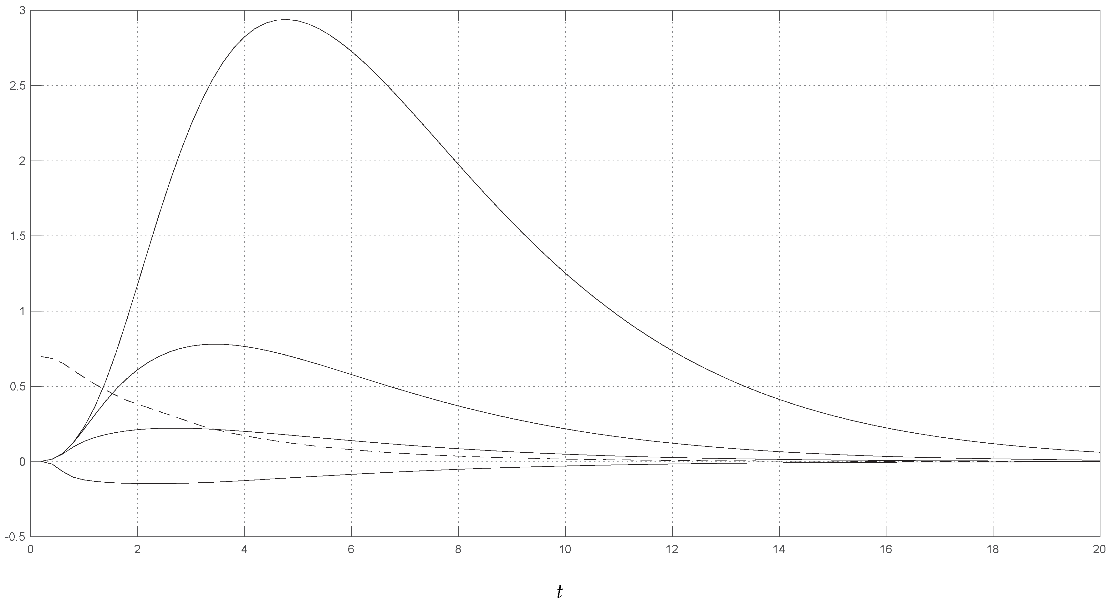
For the numerical example, we considered $\rho =3/10$ and $\alpha =3$. Figure 2 shows the numerical results. The dashed curve indicates the saddlepoint approximation ${\overline{G}}_Z\left(t\right)$ to the s.f., cf. (22), for all relevant values of t. The four solid curves of Figure 2 show the approximation to the s.f.s. ${\tilde{\tau }}_Z(t;x,F)$, for the perturbation points $x=1/2,3/2,3,7$, and for relevant values of t. The highest curves correspond to the largest values of x. The numerical evaluation of the above series representations of m.g.f. and c.g.f. does not give any particular problem: after only a few summands, numerical convergence is obtained. We note that the numerical results are similar to the ones of the Poisson-gamma aggregate loss of Section 3.1. Additionally, as with the Poisson-gamma model, the approximate s.f.s. can be computed very quickly. Thus, it can be conveniently applied to practical problems and it provides an additional indicator of the reliability of the model under uncertainty.

Figure 2. Geometric with $\rho =3/10$ compound sum of independent Weibull with $\alpha =3$ random variables. Dashed curve: s.f. Continuous curve, from lowest to highest curve: approximate stabilities for perturbation points $x=1/2,3/2,3,7$, respectively.

Appendix A.1. Derivatives of the Cumulant Generating Function of the Perturbed Summand

Recall that M and K denote the m.g.f. and the c.g.f. of $X_1$. This section gives some derivatives of $K\left(v\right)$ under the $\epsilon$-perturbation, viz. of $K_{x\epsilon }\left(v\right)=\log ((1-\epsilon )M\left(v\right)+\epsilon {\mathrm{e}}^{vx})$, w.r.t. to v and $\epsilon$. The results are the following:

$$\begin{array}{cc}\hfill \frac{\partial }{\partial \epsilon }{K}_{x\epsilon }\left(v\right)& =\frac{{\mathrm{e}}^{vx}-M\left(v\right)}{(1-\epsilon )M\left(v\right)+\epsilon {\mathrm{e}}^{vx}},\hfill \end{array}$$

$$\begin{array}{cc}\hfill {\dot{K}}_x\left(v\right)& =\frac{{\mathrm{e}}^{vx}}{M\left(v\right)}-1={\mathrm{e}}^{vx-K\left(v\right)}-1,\hfill \end{array}$$

(A1)

$$\begin{array}{cc}\hfill K_{x\epsilon }^{\prime }\left(v\right)& =\frac{\left(1-\epsilon \right)M^{\prime }\left(v\right)+\epsilon x{\mathrm{e}}^{vx}}{\left(1-\epsilon \right)M\left(v\right)+\epsilon {\mathrm{e}}^{vx}},\hfill \end{array}$$

$$\begin{array}{cc}\hfill \frac{\partial }{\partial \epsilon }{K}_{x\epsilon }^{\prime }\left(v\right)& =\frac{-M^{\prime }\left(v\right)+x{\mathrm{e}}^{vx}}{\left(1-\epsilon \right)M\left(v\right)+\epsilon {\mathrm{e}}^{vx}}-\frac{\left(\left(1-\epsilon \right)M^{\prime }\left(v\right)+\epsilon x{\mathrm{e}}^{vx}\right)\left(-M\left(v\right)+{\mathrm{e}}^{vx}\right)}{{\left(\left(1-\epsilon \right)M\left(v\right)+\epsilon {\mathrm{e}}^{vx}\right)}^2},\hfill \end{array}$$

$$\begin{array}{cc}\hfill {\dot{K}}_x^{\prime }\left(v\right)& =\frac{{\mathrm{e}}^{vx}\left(M\left(v\right)x-M^{\prime }\left(v\right)\right)}{M^2\left(v\right)}={\mathrm{e}}^{vx-K\left(v\right)}(x-K^{\prime }\left(v\right)),\hfill \end{array}$$

(A2)

$$\begin{array}{cc}\hfill K_{x\epsilon }^{″}\left(v\right)& =\frac{\left(1-\epsilon \right)M^{″}\left(v\right)+\epsilon x^2{\mathrm{e}}^{\mathit{vx}}}{\left(1-\epsilon \right)M\left(v\right)+\epsilon {\mathrm{e}}^{vx}}-\frac{{\left(\left(1-\epsilon \right)M^{\prime }\left(v\right)+\epsilon x{\mathrm{e}}^{vx}\right)}^2}{{\left(\left(1-\epsilon \right)M\left(v\right)+\epsilon {\mathrm{e}}^{vx}\right)}^2},\hfill \end{array}$$

$$\begin{array}{cc}\hfill \frac{\partial }{\partial \epsilon }{K}_{x\epsilon }^{″}\left(v\right)=& \frac{-M^{″}\left(v\right)+x^2{\mathrm{e}}^{\mathit{vx}}}{\left(1-\epsilon \right)M\left(v\right)+\epsilon {\mathrm{e}}^{vx}}-\frac{\left(\left(1-\epsilon \right)M^{″}\left(v\right)+\epsilon x^2{\mathrm{e}}^{\mathit{vx}}\right)\left(-M\left(v\right)+{\mathrm{e}}^{vx}\right)}{{\left(\left(1-\epsilon \right)M\left(v\right)+\epsilon {\mathrm{e}}^{vx}\right)}^2}\hfill \\ & -2\frac{\left(\left(1-\epsilon \right)M^{\prime }\left(v\right)+\epsilon x{\mathrm{e}}^{vx}\right)\left(-M^{\prime }\left(v\right)+x{\mathrm{e}}^{vx}\right)}{{\left(\left(1-\epsilon \right)M\left(v\right)+\epsilon {\mathrm{e}}^{vx}\right)}^2}\hfill \\ & +2\frac{{\left(\left(1-\epsilon \right)M^{\prime }\left(v\right)+\epsilon x{\mathrm{e}}^{vx}\right)}^2\left(-M\left(v\right)+{\mathrm{e}}^{vx}\right)}{{\left(\left(1-\epsilon \right)M\left(v\right)+\epsilon {\mathrm{e}}^{vx}\right)}^3},\hfill \end{array}$$

and

$$\begin{array}{cc}\hfill {\dot{K}}_x^{″}\left(v\right)& =\frac{M^2\left(v\right)x^2{\mathrm{e}}^{\mathit{vx}}-M^{″}\left(v\right)M\left(v\right){\mathrm{e}}^{vx}-2M\left(v\right)M^{\prime }\left(v\right)x{\mathrm{e}}^{vx}+2{\left(M^{\prime }\left(v\right)\right)}^2{\mathrm{e}}^{vx}}{M^3\left(v\right)}\hfill \\ & ={\mathrm{e}}^{vx-K\left(v\right)}({(x-K^{\prime }\left(v\right))}^2-K^{″}\left(v\right)).\hfill \end{array}$$

(A3)

Appendix A.2. Derivatives of the Cumulant Generating Function of the Perturbed Compound Sum

Recall that $M_N$, K, and $K_{Z_0}$ denote the m.g.f. of N and the c.g.f. of $X_1$ and of $Z_0$. This section gives some derivatives of $K_{Z_0}\left(v\right)$ under $\epsilon$-perturbation of the distribution of $X_1$, viz. of $K_{Z_{0}x\epsilon }\left(v\right)=\log \left(M_N\left(K_{x\epsilon }\left(v\right)\right)-p_0\right)-\log \left(1-p_0\right)$, w.r.t. to v and $\epsilon$. The following results are expressed in terms of the derivatives of Appendix A.1:

$$\begin{array}{cc}\hfill \frac{\partial }{\partial \epsilon }{K}_{Z_{0}x\epsilon }\left(v\right)& =\frac{M_N^{\prime }\left(K_{x\epsilon }\left(v\right)\right)\frac{\partial }{\partial \epsilon }{K}_{x\epsilon }\left(v\right)}{M_N\left(K_{x\epsilon }\left(v\right)\right)-p_0},\hfill \end{array}$$

$$\begin{array}{cc}\hfill {\dot{K}}_{Z_{0}x}\left(v\right)& =\frac{M_N^{\prime }\left(K\left(v\right)\right){\dot{K}}_x\left(v\right)}{M_N\left(K\left(v\right)\right)-p_0},\hfill \end{array}$$

(A4)

$$\begin{array}{cc}\hfill K_{Z_{0}x\epsilon }^{\prime }\left(v\right)& =\frac{M_N^{\prime }\left(K_{x\epsilon }\left(v\right)\right)K_{x\epsilon }^{\prime }\left(v\right)}{M_N\left(K_{x\epsilon }\left(v\right)\right)-p_0},\hfill \end{array}$$

$$\begin{array}{cc}\hfill \frac{\partial }{\partial \epsilon }{K}_{Z_{0}x\epsilon }^{\prime }\left(v\right)=& \frac{M_N^{″}\left(K_{x\epsilon }\left(v\right)\right)\frac{\partial }{\partial \epsilon }{K}_{x\epsilon }\left(v\right)K_{x\epsilon }^{\prime }\left(v\right)}{M_N\left(K_{x\epsilon }\left(v\right)\right)-p_0}+\frac{M_N^{\prime }\left(K_{x\epsilon }\left(v\right)\right)\frac{\partial }{\partial \epsilon }{K}_{x\epsilon }^{\prime }\left(v\right)}{M_N\left(K_{x\epsilon }\left(v\right)\right)-p_0}\hfill \\ & -\frac{{\left(M_N^{\prime }\left(K_{x\epsilon }\left(v\right)\right)\right)}^2{K}_{x\epsilon }^{\prime }\left(v\right)\frac{\partial }{\partial \epsilon }{K}_{x\epsilon }\left(v\right)}{{\left(M_N\left(K_{x\epsilon }\left(v\right)\right)-p_0\right)}^2},\hfill \end{array}$$

$$\begin{array}{cc}\hfill {\dot{K}}_{Z_{0}x}^{\prime }\left(v\right)& =\frac{M_N^{″}\left(K\left(v\right)\right){\dot{K}}_x\left(v\right)K^{\prime }\left(v\right)}{M_N\left(K\left(v\right)\right)-p_0}+\frac{M_N^{\prime }\left(K\left(v\right)\right){\dot{K}}_x^{\prime }\left(v\right)}{M_N\left(K\left(v\right)\right)-p_0}-\frac{{\left(M_N^{\prime }\left(K\left(v\right)\right)\right)}^2{K}^{\prime }\left(v\right){\dot{K}}_x\left(v\right)}{{\left(M_N\left(K\left(v\right)\right)-p_0\right)}^2},\hfill \end{array}$$

(A5)

$$\begin{array}{cc}\hfill K_{Z_{0}x\epsilon }^{″}\left(v\right)& =\frac{M_N^{″}\left(K_{x\epsilon }\left(v\right)\right){\left(K_{x\epsilon }^{\prime }\left(v\right)\right)}^2}{M_N\left(K_{x\epsilon }\left(v\right)\right)-p_0}+\frac{M_N^{\prime }\left(K_{x\epsilon }\left(v\right)\right)K_{x\epsilon }^{″}\left(v\right)}{M_N\left(K_{x\epsilon }\left(v\right)\right)-p_0}-\frac{{\left(M_N^{\prime }\left(K_{x\epsilon }\left(v\right)\right)\right)}^2{\left(K_{x\epsilon }^{\prime }\left(v\right)\right)}^2}{{\left(M_N\left(K_{x\epsilon }\left(v\right)\right)-p_0\right)}^2},\hfill \end{array}$$

(A6)

$$\begin{array}{cc}\hfill \frac{\partial }{\partial \epsilon }{K}_{Z_{0}x\epsilon }^{″}\left(v\right)=& \frac{M_N^{‴}\left(K_{x\epsilon }\left(v\right)\right)\frac{\partial }{\partial \epsilon }{K}_{x\epsilon }\left(v\right){\left(K_{x\epsilon }^{\prime }\left(v\right)\right)}^2}{M_N\left(K_{x\epsilon }\left(v\right)\right)-p_0}+2\frac{M_N^{″}\left(K_{x\epsilon }\left(v\right)\right)K_{x\epsilon }^{\prime }\left(v\right)\frac{\partial }{\partial \epsilon }{K}_{x\epsilon }^{\prime }\left(v\right)}{M_N\left(K_{x\epsilon }\left(v\right)\right)-p_0}\hfill \\ & -3\frac{M_N^{″}\left(K_{x\epsilon }\left(v\right)\right){\left(K_{x\epsilon }^{\prime }\left(v\right)\right)}^2{M}_N^{\prime }\left(K_{x\epsilon }\left(v\right)\right)\frac{\partial }{\partial \epsilon }{K}_{x\epsilon }\left(v\right)}{{\left(M_N\left(K_{x\epsilon }\left(v\right)\right)-p_0\right)}^2}\hfill \\ & +\frac{M_N^{″}\left(K_{x\epsilon }\left(v\right)\right)\frac{\partial }{\partial \epsilon }{K}_{x\epsilon }\left(v\right)K_{x\epsilon }^{″}\left(v\right)}{M_N\left(K_{x\epsilon }\left(v\right)\right)-p_0}+\frac{M_N^{\prime }\left(K_{x\epsilon }\left(v\right)\right)\frac{\partial }{\partial \epsilon }{K}_{x\epsilon }^{″}\left(v\right)}{M_N\left(K_{x\epsilon }\left(v\right)\right)-p_0}\hfill \\ & -\frac{{\left(M_N^{\prime }\left(K_{x\epsilon }\left(v\right)\right)\right)}^2{K}_{x\epsilon }^{″}\left(v\right)\frac{\partial }{\partial \epsilon }{K}_{x\epsilon }\left(v\right)}{{\left(M_N\left(K_{x\epsilon }\left(v\right)\right)-p_0\right)}^2}-2\frac{{\left(M_N^{\prime }\left(K_{x\epsilon }\left(v\right)\right)\right)}^2{K}_{x\epsilon }^{\prime }\left(v\right)\frac{\partial }{\partial \epsilon }{K}_{x\epsilon }^{\prime }\left(v\right)}{{\left(M_N\left(K_{x\epsilon }\left(v\right)\right)-p_0\right)}^2}\hfill \\ & +2\frac{{\left(M_N^{\prime }\left(K_{x\epsilon }\left(v\right)\right)\right)}^3{\left(K_{x\epsilon }^{\prime }\left(v\right)\right)}^2\frac{\partial }{\partial \epsilon }{K}_{x\epsilon }\left(v\right)}{{\left(M_N\left(K_{x\epsilon }\left(v\right)\right)-p_0\right)}^3},\hfill \end{array}$$

$$\begin{array}{cc}\hfill {\dot{K}}_{Z_{0}x}^{″}\left(v\right)=& \frac{M_N^{‴}\left(K\left(v\right)\right){\dot{K}}_x\left(v\right){\left(K^{\prime }\left(v\right)\right)}^2}{M_N\left(K\left(v\right)\right)-p_0}+2\frac{M_N^{″}\left(K\left(v\right)\right)K^{\prime }\left(v\right){\dot{K}}_x^{\prime }\left(v\right)}{M_N\left(K\left(v\right)\right)-p_0}\hfill \\ & -3\frac{M_N^{″}\left(K\left(v\right)\right){\left(K^{\prime }\left(v\right)\right)}^2{M}_N^{\prime }\left(K\left(v\right)\right){\dot{K}}_x\left(v\right)}{{\left(M_N\left(K\left(v\right)\right)-p_0\right)}^2}+\frac{M_N^{″}\left(K\left(v\right)\right){\dot{K}}_x\left(v\right)K^{″}\left(v\right)}{M_N\left(K\left(v\right)\right)-p_0}\hfill \\ & +\frac{M_N^{\prime }\left(K\left(v\right)\right){\dot{K}}_x^{″}\left(v\right)}{M_N\left(K\left(v\right)\right)-p_0}-\frac{{\left(M_N^{\prime }\left(K\left(v\right)\right)\right)}^2{K}^{″}\left(v\right){\dot{K}}_x\left(v\right)}{{\left(M_N\left(K\left(v\right)\right)-p_0\right)}^2}\hfill \\ & -2\frac{{\left(M_N^{\prime }\left(K\left(v\right)\right)\right)}^2{K}^{\prime }\left(v\right){\dot{K}}_x^{\prime }\left(v\right)}{{\left(M_N\left(K\left(v\right)\right)-p_0\right)}^2}+2\frac{{\left(M_N^{\prime }\left(K\left(v\right)\right)\right)}^3{\left(K^{\prime }\left(v\right)\right)}^2{\dot{K}}_x\left(v\right)}{{\left(M_N\left(K\left(v\right)\right)-p_0\right)}^3},\hfill \end{array}$$

(A7)

and

$$\begin{array}{cc}\hfill K_{Z_0}^{‴}\left(v\right)=& \frac{M_N^{‴}\left(K\left(v\right)\right){\left(K^{\prime }\left(v\right)\right)}^3}{M_N\left(K\left(v\right)\right)-p_0}+3\frac{M_N^{″}\left(K\left(v\right)\right)K^{\prime }\left(v\right)K^{″}\left(v\right)}{M_N\left(K\left(v\right)\right)-p_0}\hfill \\ & -3\frac{M_N^{″}\left(K\left(v\right)\right){\left(K^{\prime }\left(v\right)\right)}^3{M}_N^{\prime }\left(K\left(v\right)\right)}{{\left(M_N\left(K\left(v\right)\right)-p_0\right)}^2}+\frac{M_N^{\prime }\left(K\left(v\right)\right)K^{‴}\left(v\right)}{M_N\left(K\left(v\right)\right)-p_0}\hfill \\ & -3\frac{{\left(M_N^{\prime }\left(K\left(v\right)\right)\right)}^2{K}^{″}\left(v\right)K^{\prime }\left(v\right)}{{\left(M_N\left(K\left(v\right)\right)-p_0\right)}^2}+2\frac{{\left(M_N^{\prime }\left(K\left(v\right)\right)\right)}^3{\left(K^{\prime }\left(v\right)\right)}^3}{{\left(M_N\left(K\left(v\right)\right)-p_0\right)}^3}.\hfill \end{array}$$

(A8)

References

- Asmussen, Soren, and Hansjorg Albrecher. 2010. Ruin Probabilities, 2nd ed. Singapore: World Scientific. [Google Scholar]
- Asmussen, Soren, and Peter W. Glynn. 2007. Stochastic Simulation. Algorithms and Analysis. New York: Springer. [Google Scholar]
- Asmussen, Soren, and Reuven Y. Rubinstein. 1999. Sensitivity analysis of insurance risk models via simulation. Management Science 45: 1125–41. [Google Scholar] [CrossRef]
- Daniels, Henry Ellis. 1954. Saddlepoint approximations in statistics. Annals of Mathematical Statistics 25: 631–50. [Google Scholar] [CrossRef]
- Field, Christopher A., and Elvezio Ronchetti. 1985. A tail area influence function and its application to testing. Sequential Analysis 4: 19–41. [Google Scholar] [CrossRef]
- Gatto, Riccardo, and Michael Mosimann. 2012. Four approaches to compute the probability of ruin in the compound Poisson risk process with diffusion. Mathematical and Computer Modelling 55: 1169–85. [Google Scholar] [CrossRef]
- Gatto, Riccardo, and Chantal Peeters. 2015. Saddlepoint approximations to sensitivities of tail probabilities of random sums and comparisons with Monte Carlo estimators. Journal of Statistical Computation and Simulation 85: 641–59. [Google Scholar] [CrossRef]
- Grübel, Rudolf. 1989. Stochastic models as functionals: Some remarks on the renewal case. Journal of Applied Probability 26: 296–303. [Google Scholar] [CrossRef]
- Hampel, Frank Rudolf, Elvezio M. Ronchetti, Peter Rousseeuw, and Werner Alfred Stahel. 1986. Robust Statistics. The Approach Based on Influence Functions. New York: Wiley & Sons. [Google Scholar]
- Jensen, Jens Ledet. 1995. Saddlepoint Approximations. New York: Oxford University Press. [Google Scholar]
- Lugannani, Robert, and Stephen Rice. 1980. Saddle point approximation for the distribution of the sum of independent random variables. Advances in Applied Probability 12: 475–90. [Google Scholar] [CrossRef]
- Politis, Konstadinos. 2006. A functional approach for ruin probabilities. Stochastic Models 22: 509–36. [Google Scholar] [CrossRef]
© 2018 by the author. Licensee MDPI, Basel, Switzerland. This article is an open access article distributed under the terms and conditions of the Creative Commons Attribution (CC BY) license (http://creativecommons.org/licenses/by/4.0/).