The Impact of Sovereign Yield Curve Differentials on Value-at-Risk Forecasts for Foreign Exchange Rates

Abstract

A functional ARMA-GARCH model for predicting the value-at-risk of the EURUSD exchange rate is introduced. The model implements the yield curve differentials between EUR and the US as exogenous factors. Functional principal component analysis allows us to use the information of basically the whole yield curve in a parsimonious way for exchange rate risk prediction. The data analyzed in our empirical study consist of the EURUSD exchange rate and the EUR- and US-yield curves from 15 August 2005–30 September 2016. As a benchmark, we take an ARMA-GARCH and an ARMAX-GARCHX with the 2y-yield difference as the exogenous variable and compare the forecasting performance via likelihood ratio tests. However, while our model performs better in one situation, it does not seem to improve the performance in other setups compared to its competitors.

1. Introduction

Forecasting foreign exchange (FX) rates and especially risk inherent in such FX markets is of crucial importance to companies and individuals of Wall Street as well as Main Street. In particular, for portfolio managers, corporations and the like, managing FX risk is essential. Accordingly, a large amount of research is available in this field.

The work in, e.g., Meese and Rogoff (1983) analyzed FX rate models developed in the 1970s and came to the conclusion that these did not perform better than random walks, which exemplifies the difficulty in modeling spot FX rates. Even the addition of macroeconomic variables like expected inflation and interest rate differentials (among others) did not lead to significant improvements. Similar findings have been reported by Campbell and Clarida (1987), Meese and Rogoff (1988), Coughlin and Koedijk (1990), Edison and Pauls (1993), Chinn and Meese (1995) and Frankel and Rose (1995). Having said that, others disagree with the findings of the previous authors; see for instance Bjørnland and Hungnes (2006), Ang and Chen (2010), Chen and Tsang (2013) and Grisse and Nitschka (2015).

However, the above discussion might not be that surprising as it basically boils down to the question whether one believes in the efficient market hypothesis of Fama (1970). Nevertheless, forecasting volatility, which is of crucial importance to risk management, is another matter: e.g., Baillie and Bollerslev (1991) proposed a seasonal GARCH setup to model intraday FX rate volatility. In their findings, they experienced volatility to follow patterns that were very much alike over various hours of the day and to show a notable amount of serial correlation. For volatility based on daily FX spot levels, Vilasuso (2002) employed the fractionally-integrated GARCH by Baillie et al. (1996) and reported a significant improvement in out-of-sample performance with respect to mean squared and mean absolute errors, as well as to accuracy, in comparison to the simpler GARCH or IGARCH models.

Moreover, the assumption of financial market log-returns being normally distributed has been criticized for a long time. Therefore, Hull and White (1998) introduced a model to estimate value-at-risk (VaR) that does not postulate a normal distribution, producing promising results. A similar approach was also adopted by Mittnik and Paolella (2000) and Kuester et al. (2006). The latter were able to identify a clear overall winner in their comparison of different VaR forecasting techniques, which turns out to be a combination of a heavy-tailed GARCH filter and extreme value theory approach.

Another approach to improve FX volatility and risk forecasting performance is to invoke external factors, as carried out by, e.g., Benavides and Capistràn (2012), who made use of implied volatility information from option prices. In line with the above-mentioned discussion on macroeconomic variables for spot models, several authors have incorporated yield curve information into FX risk models, as well; cf. Dominguez (1998), Neely (1999), Markiewicz (2012), Kočenda and Poghosyan (2009) and Ichiue and Koyama (2011). See furthermore Morana (2009), who analyzed the influence of macroeconomics, among which were interest rates, on FX rate volatility. When it comes to explicitly forecasting FX rate volatility employing macro variables, we mention the usage of neural networks as investigated, e.g., by Dunis and Huang (2002), who compared their model to GARCH models and reported superior results with their setup, in which they included yield curve data, among other inputs. Furthermore, we have Bauwens and Sucarrat (2010), who employed, among other macro variables, interest rates for exchange rate volatility forecasts.

For a more general analysis on the influence of macroeconomic factors on volatility forecasts, we refer to Christiansen et al. (2012), who found, in particular, more evidence for an influence of macro variables on FX rate volatility forecasts. Finally, the use of Euro deposit rates as a measure of performance for forecasts of FX volatility was introduced in West et al. (1993).

However, to the best of our knowledge, no one has yet investigated if using the complete sovereign yield curve differential (in contrast to just some specific maturities) does effectively improve VaR forecasting. The idea of using such functional exogenous parts in a GARCHX setup for volatility modeling has been introduced before by Fuest and Mittnik (2015). We extend this approach to an ARMAX-GARCHX-type setup, which allows the exogenous yield curve differential to influence both return and volatility.

In particular, we want to investigate the following for EURUSD as our lead example: Does the complete yield curve differential have significant effects on daily FX returns predictions? Does it improve VaR forecasts? Does the proposed mathematical machinery pay off when comparing it to a standard ARMA-GARCH model and an ARMAX-GARCHX with the 2y-yield difference as the exogenous variable? We will investigate these questions by the analysis of confidence intervals and by the evaluation of likelihood ratio tests.

Dealing with functional data, we conclude this section with a short survey on functional time series research. A comprehensive treatment of functional data analysis (FDA) is Ramsay and Silverman (2005). Models for functional time series have been pioneered in the seminal treatment of Bosq (2000), where a generalization of pure autoregressive models to the functional case was developed. More recently, dimension reduction techniques (Hörmann and Kokoszka 2010) and dynamic models based on such techniques (Aue et al. 2015; Hyndman and Shang 2009) have been proposed and investigated. The work in Klepsch et al. (2017) proposed functional ARMA models and Hörmann et al. (2013) a functional version of the ARCH model. Functional time series approaches have very recently also been employed to model yield curve dynamics Kowal et al. (2017a, 2017b). In our study, however, a scalar time series is of primary interest. The idea to map the full information inherent in functional data to first- and, possibly, higher-order moments of the conditional distribution of a scalar time series has been put forward in Fuest and Mittnik (2015) and Brockhaus et al. (2017).

The remainder of this paper is structured as follows: In Section 2, we will present the data used for our analysis and discuss the construction of the EUR- and US-yield curve. Section 3 starts with a short introduction to functional principal component analysis, which is followed by presenting the method of implementation used in this investigation, as shown in Ramsay and Silverman (2005). Having described the background mathematics, we introduce our model and the estimation procedure applied later. In Section 4, we present our estimation results and discuss the implications. Finally we conduct one-day VaR forecasts and compare these to predictions coming from the competing models.

All calculations have been performed with MATLAB (R2014b, MathWorks, Natick, MA, USA) using the financial econometrics toolbox by Sheppard (2013) and the functional data toolbox by Ramsay (2014).

2. Data

In this section, we shall briefly present the data used in our analysis to come. In particular, the present paper considers daily prices of the EURUSD exchange rate and daily levels of the EUR- and US-yield curves. Our time period ranges from 15 August 2005–30 September 2016, which leaves us with a total sample of $n=2905$ observations. Figure 1 shows the daily log-returns for the FX series, while Figure 2 visualizes the yield curve differential via the 2y-yields.

To be precise, we constructed the yield curve for Europe by using the EONIA (European overnight index average) offered rate for a maturity of 0 and the overnight index swap (OIS) rates based on EONIA with maturities of 1–12 months, 15 months, 18 months, 21 months and 2–10 years. The EONIA for the shortest maturity and the OIS for longer maturities are representative choices for constructing a Euro yield curve (cf. FBE (2008)), since overnight index swaps have established themselves as a benchmark proxy for the risk-free rate. (cf. Hull and White (2012) and Filipović and Trolle (2013), among others.)

For the US-yield curve, we used the federal funds rate for a maturity of 0 and yields obtained from US government bonds with maturities of 1, 3 and 6 months and 1–5, 7 and 10 years. Figure 3 visualizes the varying shape of the resulting curves. Finally, we converted the obtained discrete yield curves into functional data by using cubic B-splines. In the remainder of this paper, the terms “sovereign rate curve”, “rate curve” and “yield curve” will be used interchangeably.

3. Theory and Methods

In this section, we show how all the information contained in the yield curve at a given point in time can be mapped to the mean and variance parameters of the conditional distribution of exchange rate returns. The core technique we need for this purpose is functional principal component analysis (FPCA). We will sketch the theory and present the method of implementation that we used for our data, the implementation via basis expansion. As we will show, the estimated eigenfunctions from FPCA are also used to conveniently represent and estimate the functional parameters of our model. We will heavily draw on Ramsay and Silverman (2005), as well as Hörmann and Kokoszka (2012). For details on FPCA theory, we refer to the former and for a comprehensive treatment of functional regression models to the latter.

3.1. Functional Principal Components

We consider a stochastic process ${\left(x_t\right)}_{t\in \mathcal{T}}.$ In order to simplify notation, we use lowercase letters for the processes, as well as for the realizations. For an ordered finite index set $\mathcal{T}$, we index our observations as $x_1,\dots ,x_{\left|\mathcal{T}\right|}.$

Now, consider the $x_t$ as elements of the Hilbert space ${\mathcal{L}}^2\left([0,M]\right).$ The Hilbert space ${\mathcal{L}}^2\left([0,M]\right)$ is endowed with the inner product:

$$〈x,y〉={\int }_0^{M}x\left(s\right)y\left(s\right)\mathrm{d}s,\forall x,y\in {\mathcal{L}}^2\left([0,M]\right),$$

so we have that $x_t$ is square integrable.

Our curve valued process $x_t$ exhibits a mean function, $\mu \left(s\right)=\mathbb{E}\left(x_t\left(s\right)\right)$, and a covariance operator,

$$\mathcal{C}:{\mathcal{L}}^2\left([0,M]\right)⟶{\mathcal{L}}^2\left([0,M]\right),f\mapsto {\int }_0^M\mathrm{Cov}(r,s)f\left(r\right)\mathrm{d}r.$$

with covariance kernel $\mathrm{Cov}(r,s)=\mathrm{Covariance}(x_t\left(r\right),x_t\left(s\right)).$

Both mean function and covariance kernel are assumed to be constant over time $t\in \mathcal{T}$. Further note that for a $z\in {\mathcal{L}}^2\left([0,M]\right)$, we have $\mathcal{C}\left(z\right)=\mathbb{E}\left[〈x-\mu ,z〉(x-\mu )\right].$

Our goal is to find orthonormal weight functions, ${\gamma }_k\in {\mathcal{L}}^2\left([0,M]\right)$, maximizing the unconditional variance of the scores ${\xi }_k=〈{\gamma }_k,x_t-\mu 〉={\int }_0^M{\gamma }_k\left(s\right)(x_t\left(s\right)-\mu \left(s\right))\mathrm{d}s$, i.e.,

$$\mathrm{Var}\left({\xi }_k\right)={\int }_0^M{\int }_0^M{\gamma }_k\left(r\right)\mathrm{Cov}(r,s){\gamma }_k\left(s\right)\mathrm{d}r\mathrm{d}s.$$

(1)

The weight functions, ${\gamma }_k$, are subject to orthonormality constraints, i.e., to:

$$〈{\gamma }_k,{\gamma }_l〉={\int }_0^M{\gamma }_k\left(s\right){\gamma }_l\left(s\right)\mathrm{d}s=\left\{\begin{array}{cc}1\hfill & \mathrm{if}k=l\hfill \\ 0\hfill & \mathrm{if}k\ne l.\hfill \end{array}\right.$$

(2)

Then, the weight functions ${\gamma }_k$ happen to be the eigenfunctions of the covariance operator $\mathcal{C}$. $\mathcal{C}$ is a bounded, symmetric, positive operator, and its eigenfunctions ${\gamma }_k$ form an orthonormal basis of ${\mathcal{L}}^2\left([0,M]\right).$ The so-called Fredholm (integral) equations:

$${\int }_0^M\mathrm{Cov}(r,s)f\left(s\right)\mathrm{d}s={\lambda }_{k}f\left(r\right)$$

(3)

give us the ${\gamma }_k$, which are ordered ascendingly as their corresponding eigenvalues ${\lambda }_1\ge {\lambda }_2\ge \cdots \ge 0.$ Finally, these eigenfunctions maximize (1).

Further note that $\mathrm{Cov}(r,s)$ is a Mercer kernel. In particular, this means that it can be represented in terms of the eigenvectors, ${\gamma }_k$, and the eigenvalues, ${\lambda }_k$, of the covariance operator $\mathcal{C}$,

$$\mathrm{Cov}(r,s)=\sum _{k=1}^{\infty }{\lambda }_k{\gamma }_k\left(r\right){\gamma }_k\left(s\right).$$

Now, applying the theorem of Karhunen–Loève, we are able to represent the centered (yield) curve process, $x_t-\mu$, via its eigenbasis ${\left({\gamma }_k\right)}_k$,

$$x_t-\mu =\sum _{k=1}^{\infty }{\xi }_{k,t}{\gamma }_k,$$

where the eigenfunctions, ${\gamma }_k$, are the eigenvectors of the linear operator $\mathcal{C}$, and the scores, ${\xi }_{k,t}$, have the properties:

$$\mathbb{E}\left({\xi }_{k,t}\right)=0,\mathrm{Var}\left({\xi }_{k,t}\right)=\mathbb{E}({\xi }_{k,t}^2)={\lambda }_k\mathrm{and}\mathbb{E}({\xi }_{k,t}·{\xi }_{l,t})=0\mathrm{for}k\ne l.$$

Recall that the eigenvalues, ${\lambda }_k$, are ordered in a non-decreasing order, so that the functional principal components are sorted by their contribution to the variation of the $x_t$’s.

Let K be the smallest number necessary to explain a certain amount of the curves’ total variation, then we can approximate our curve by:

$$x_t\approx \mu +\sum _{k=1}^K{\xi }_{k,t}{\gamma }_k.$$

Consider a yield curve $x_t:\mathrm{Maturities}\to \mathrm{Yields},$ observed at time t. The above result means that we can approximate the information inherent in the yield curve over the entire range of observed maturities by a (possibly small) set of K scalar values. Note, however, that real-world observed yield curve data are only available for certain maturities m, which are, in most cases, not even structured in an equidistant way.1 As is common practice in functional data analysis, we use spline interpolation of the observed yields to obtain equidistant maturities.

The resulting approximations of the yield curve can then be implemented and analyzed in our functional principal component analysis. There are several possibilities of implementing FPCA, of which we chose the method of “basis expansion” in our application, as is presented in Ramsay and Silverman (2005), which we briefly describe in the following.

We start by expressing our data, given by a matrix:

$$\left(\begin{array}{cccc}{x}_1\left(0\right)& \cdots & \cdots & x_1\left(M\right)\\ ⋮& \ddots & \ddots & ⋮\\ ⋮& \ddots & \ddots & ⋮\\ x_{\left|\mathcal{T}\right|}\left(0\right)& \cdots & \cdots & x_{\left|\mathcal{T}\right|}\left(M\right)\end{array}\right),$$

in terms of a basis $\mathcal{B}$ in order to obtain a curve $x_t.$ Thus, for each $t\in \mathcal{T}$, we can represent $x_t$ by:

$$x_t\left(s\right)=\sum _{k=1}^{\left|\mathcal{B}\right|}{c}_{t,k}{\psi }_k\left(s\right),$$

which is equivalent to:

$$\left(\begin{array}{c}{x}_1\\ ⋮\\ ⋮\\ x_{\left|\mathcal{T}\right|}\end{array}\right)=\mathit{C}·\mathit{\psi }=\left(\begin{array}{cccc}{c}_{1,1}& \cdots & \cdots & c_{1,\left|\mathcal{B}\right|}\\ ⋮& \ddots & \ddots & ⋮\\ ⋮& \ddots & \ddots & ⋮\\ c_{\left|\mathcal{T}\right|,1}& \cdots & \cdots & c_{\left|\mathcal{T}\right|,\left|\mathcal{B}\right|}\end{array}\right)·\left(\begin{array}{c}{\psi }_1\\ ⋮\\ ⋮\\ {\psi }_{\left|\mathcal{B}\right|}\end{array}\right),$$

where $\left|\mathcal{B}\right|$ denotes the number of basis functions of the chosen basis $\mathcal{B}.$

We then have:

$$\mathrm{Cov}(r,s)={\left|\mathcal{T}\right|}^{-1}{\mathit{\psi }\left(r\right)}^{\mathrm{T}}{\mathit{C}}^{\mathrm{T}}\mathit{C}\mathit{\psi }\left(s\right).$$

Now, define the symmetric matrix:

$$\mathit{W}={\int }_0^M\mathit{\psi }\left(s\right)\mathit{\psi }{\left(s\right)}^{\mathrm{T}}\mathrm{d}s={\left({\int }_0^M{\psi }_i\left(s\right){\psi }_j\left(s\right)\mathrm{d}s\right)}_{i,j}.$$

We assume that the eigenfunctions ${\gamma }_k$ are representable using the basis $\mathcal{B}$ in the form:

$${\gamma }_k=\sum _{l=1}^{\left|\mathcal{B}\right|}{\alpha }_{k,l}{\psi }_l={\mathit{\psi }}^{\mathrm{T}}{\alpha }_{\mathit{k}},$$

where ${\mathit{\alpha }}_{\mathit{k}}=({\alpha }_{k,1},\cdots ,{\alpha }_{k,\left|\mathcal{B}\right|}).$ Now, we express the Fredholm Equation (3) in terms of our basis $\mathcal{B}$ by considering the left-hand side of (3) with $f={\gamma }_k$,

$${\int }_0^M\mathrm{Cov}(r,s){\gamma }_k\left(s\right)\mathrm{d}s={\int }_0^M{\left|\mathcal{T}\right|}^{-1}{\mathit{\psi }\left(r\right)}^{\mathrm{T}}{\mathit{C}}^{\mathrm{T}}\mathit{C}\mathit{\psi }\left(s\right){\mathit{\psi }\left(s\right)}^{\mathrm{T}}{\mathit{\alpha }}_{\mathit{k}}\mathrm{d}s={\mathit{\psi }\left(r\right)}^{\mathrm{T}}{\left|\mathcal{T}\right|}^{-1}{\mathit{C}}^{\mathrm{T}}\mathit{C}\mathit{W}{\mathit{\alpha }}_{\mathit{k}}.$$

Employing the basis representation of ${\gamma }_k$, the Fredholm equations then form:

$${\mathit{\psi }\left(r\right)}^{\mathrm{T}}{\left|\mathcal{T}\right|}^{-1}{\mathit{C}}^{\mathrm{T}}\mathit{C}\mathit{W}{\mathit{\alpha }}_{\mathit{k}}={\lambda }_k{\mathit{\psi }\left(r\right)}^{\mathrm{T}}{\mathit{\alpha }}_{\mathit{k}}$$

and we obtain:

$${\left|\mathcal{T}\right|}^{-1}{\mathit{C}}^{\mathrm{T}}\mathit{C}\mathit{W}{\mathit{\alpha }}_{\mathit{k}}={\lambda }_k{\mathit{\alpha }}_{\mathit{k}}.$$

Considering the orthogonality correspondence:

$$〈{\gamma }_k,{\gamma }_l〉=0\iff {\mathit{\alpha }}_{\mathit{k}}^{\mathrm{T}}\mathit{W}{\mathit{\alpha }}_{\mathit{l}}=0,$$

we note that for $∥{\gamma }_k∥=1$, we have ${{\mathit{\alpha }}_{\mathit{k}}}^{\mathrm{T}}\mathit{W}{\mathit{\alpha }}_{\mathit{k}}=1,$ resulting in the same correspondence from above for normality. By defining ${\mathit{u}}_{\mathit{k}}:={\mathit{W}}^{1/2}{\mathit{\alpha }}_{\mathit{k}}$, we arrive at the symmetric eigenvalue problem:

$${\left|\mathcal{T}\right|}^{-1}{\mathit{W}}^{1/2}{\mathit{C}}^{\mathrm{T}}\mathit{C}{\mathit{W}}^{1/2}{\mathit{u}}_{\mathit{k}}={\lambda }_k{\mathit{u}}_{\mathit{k}}.$$

Solving this problem gives us the ${\mathit{u}}_{\mathit{k}}$, and in turn, we get:

$${\mathit{\alpha }}_{\mathit{k}}={\mathit{W}}^{-1/2}{\mathit{u}}_{\mathit{k}}.$$

The scores ${\xi }_{k,t}$ are then obtained by:

$${\xi }_{k,t}=〈x_t-\mathbb{E}\left(x_t\right),{\mathit{\alpha }}_{\mathit{k}}〉.$$

Next, we shortly discuss how the mean, eigenfunctions and the corresponding scores can be estimated from data. As mentioned above, we observe values of the yield curves $x_t$ on a (possibly non-equidistant) grid of maturities. By spline interpolation, we obtain a discrete version of $x_t$ on an equidistant grid of maturities $0,\dots ,M$. Therefore, the realization of each $x_t$ is an $M+1$-dimensional vector. Using interpolation, the number $J+1$ of grid points can be chosen arbitrarily, and one obtains an equidistant grid of the form $m_0=0,m_1=M/J,m_2=2M/J,\dots ,m_{J-1}=(J-1)M/J,m_J=M.$ The more complex the variation pattern of the curves, the higher J has to be chosen. For yield curves, the variation pattern is typically rather simple and the curves rather smooth, so that a moderate M should be reasonable. We found that a grid distance of one month is sufficient for our purpose, resulting in the choice $J=120.$

The estimates of the mean function and the covariance kernel are given by:

$$\widehat{\mu }\left(m_j\right)=\frac{1}{\left|\mathcal{T}\right|}\sum _{t=1}^{\left|\mathcal{T}\right|}{x}_t\left(m_j\right),m_j\in [0,M]$$

and:

$$\widehat{\mathrm{Cov}}=\frac{1}{\left|\mathcal{T}\right|}{\mathit{X}}^{c^{\mathrm{T}}}{\mathit{X}}^c,$$

where $\left|\mathcal{T}\right|$ is the number of observations (e.g., the number of observed yield curves $x_t$), ${\mathit{x}}_t={[x_t\left(0\right),\cdots ,x_t\left(M\right)]}^{\mathrm{T}},$ $\widehat{\mathit{\mu }}={[\widehat{\mu }\left(0\right),\cdots ,\widehat{\mu }\left(M\right)]}^{\mathrm{T}}$ and ${\mathit{X}}^c={[{\mathit{x}}_1-\widehat{\mathit{\mu }},\cdots ,{\mathit{x}}_{\left|\mathcal{T}\right|}-\widehat{\mathit{\mu }}]}^{\mathrm{T}}.$

In this framework, the eigenvalues ${\widehat{\lambda }}_k$ and eigenvectors ${\widehat{\gamma }}_k$ of $\widehat{\mathrm{Cov}}$ can be estimated using standard software for PCA. By means of numerical integration, we get empirical scores:

$${\widehat{\xi }}_{k,t}={\int }_0^M(x_t\left(m\right)-\widehat{\mu }\left(m\right)){\widehat{\gamma }}_k\left(m\right)\mathrm{d}m.$$

The covariance operator $\mathcal{C}$ itself can be estimated by:

$$\widehat{\mathcal{C}}\left(z\right)=\frac{1}{\left|\mathcal{T}\right|}\sum _{t=1}^{\left|\mathcal{T}\right|}〈x_t-\widehat{\mu },z〉(x_t-\widehat{\mu })\mathrm{for}z\in {\mathcal{L}}^2\left([0,M]\right).$$

3.2. Econometric Model

We now define our model, which incorporates curve-valued information into a (scalar) ARMA-GARCH framework.

Definition 1 (ARMA(1,1)FunX-logGARCH(1,1)FunX process).

Let $x_t$ be drawn from a curve-valued exogenous process. Then, $r_t$ follows an ARMA(1,1)FunX-logGARCH(1,1)FunX process if:

$$\begin{array}{ccc}\hfill r_t& =& {\displaystyle {\alpha }_0+\alpha r_{t-1}+\beta {ϵ}_{t-1}+{ϵ}_t+{\int }_0^M\lambda \left(m\right)x_{t-1}dm,}\hfill \\ \hfill {ϵ}_t& =& {\sigma }_t{e}_t,\hfill \\ \hfill log{\sigma }_t^2& =& {\displaystyle \omega +\gamma log{ϵ}_{t-1}^2+\delta log{\sigma }_{t-1}^2+{\int }_0^M\rho \left(m\right)x_{t-1}dm,}\hfill \end{array}$$

with $e_t\sim WN(0,1).$

In our case, we have:

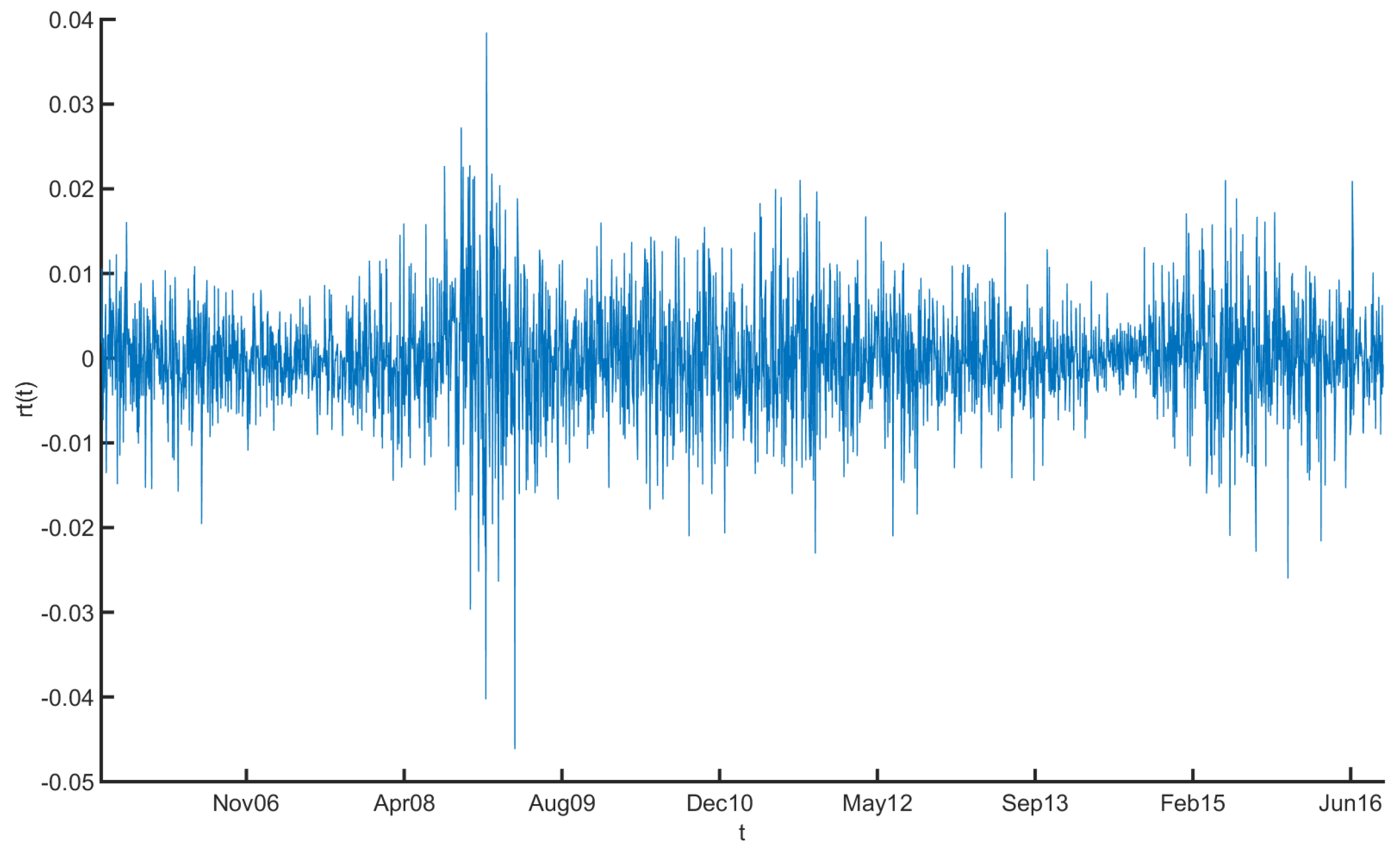
• $r_t$ is the FX rate EURUSD
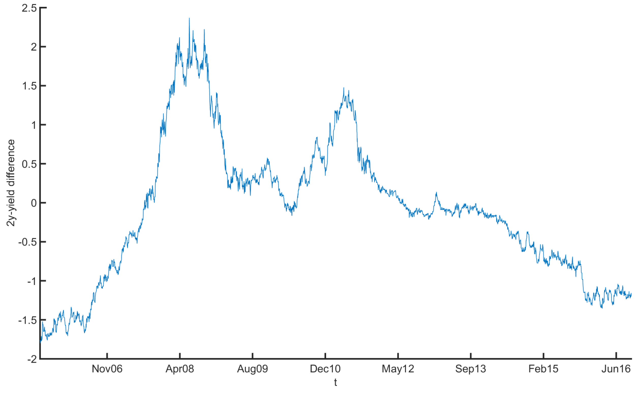
• $z_t^{\mathrm{US}}(·)$ is the sovereign rate curve for the US
• $z_t^{\mathrm{EUR}}(·)$ is the sovereign rate curve for EUR.
• $x_t(·)=z_t^{\mathrm{EUR}}(·)-z_t^{\mathrm{US}}(·)$

Estimation is rendered feasible by expressing all functional elements of the model within an ARMAX(1,1)-log-GARCHX(1,1) framework, where the X-part is given by the K-dimensional approximations of functional observations and parameters. Concerning the resulting Gaussian QML estimators, there is some asymptotic theory for the GARCHX (see Han (2015), Han and Kristensen (2014)) and ARMAX models (see Hannan et al. (1980)). However, according to Sucarrat et al. (2016), Francq et al. (2013) and Hansen et al. (2012), there is none for the log-GARCHX case.

Remark 1.

The generalization of our setup to an ARMAX(A,B)-log-GARCHX(1,1) or even an ARMAX(A,B)-log-GARCHX(C,D), allowing for an arbitrary number of lags, is straightforward. For the sake of brevity and conciseness, we will nevertheless work with the ARMAX(1,1)-log-GARCHX(1,1) case in this paper, since the novelty and core idea of our model lies within the exogenous part.

As introduced in Section 3.1, we can approximate our curve-valued process $x_t$ by its first K principal components:

$$x_t\approx \mu +\sum _{k=1}^K{\xi }_{k,t}{\gamma }_k.$$

As in Fuest and Mittnik (2015), it is convenient to assume the existence of some $K<\infty$ such that:

$$\begin{array}{ccc}\hfill {\int }_0^M\sum _{k=K+1}^{\infty }{\gamma }_k\left(m\right)x_t\left(m\right)\mathrm{d}m& =& 0\hfill \\ \hfill \iff {\int }_0^M\sum _{k=K+1}^{\infty }\sum _{l=1}^{\infty }{\gamma }_k\left(m\right){\gamma }_l\left(m\right){\xi }_{l,t}\mathrm{d}m& =& 0\hfill \\ \hfill \iff {\int }_0^M\sum _{k=K+1}^{\infty }\sum _{l=K+1}^{\infty }{\gamma }_k\left(m\right){\gamma }_l\left(m\right){\xi }_{l,t}\mathrm{d}m& =& 0.\hfill \end{array}$$

In other words, we assume that the number of principal components that actually have an effect on the return (ARMA-part) or the variance (GARCH-part) is finite. As they are ordered by their contribution to the curves’ variation, the leading K components are the ones that explain the variation best. However, there might still be dependencies between the first K and the remaining components. We (realistically) assume that these lead/lag effects of components $K+1,\cdots$ on the first K components’ scores are negligible.

Estimation of the model can then be accomplished in three steps:

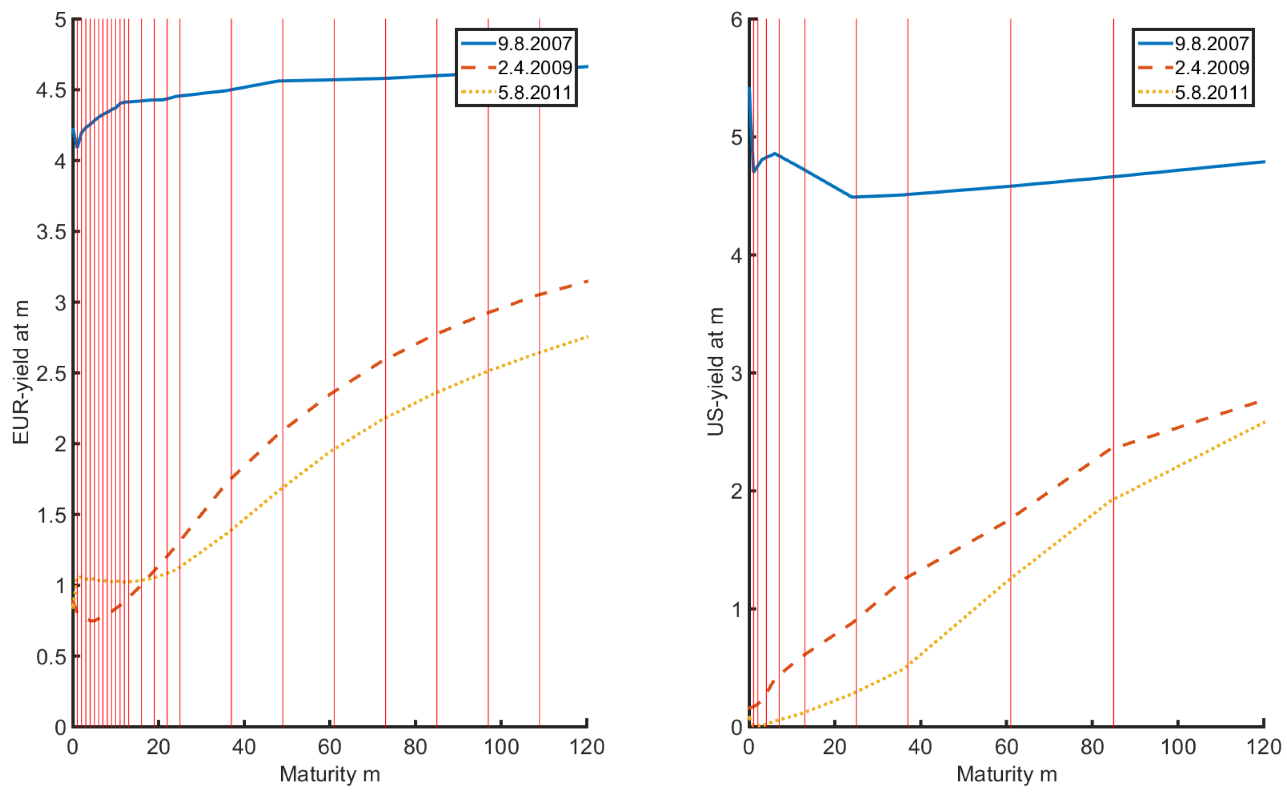
• Estimation of the curved valued process $x_t$ via an orthonormal FPC expansion:

  $${\widehat{x}}_t=\widehat{\mu }+\sum _{k=1}^K{\widehat{\xi }}_{k,t}{\widehat{\gamma }}_k,$$

  where the true values of $K,$$\mu$ and ${\gamma }_k$ are unknown and the ${\widehat{\xi }}_{k,t}$ are obtained via numerical integration (see Section 3.1).
• Estimation of the ARMA-FunX parameters using the scores ${\widehat{\xi }}_{k,t}$ for $k=1,\cdots ,K$ and $t=1,\cdots ,\left|\mathcal{T}\right|$ from Step 1 and the return data by Gaussian QML.
• Gaussian QML estimation of the GARCH-FunX parameters using the scores ${\widehat{\xi }}_{l,t}$ for $l=1,\cdots ,L$, $t=1,\cdots ,\left|\mathcal{T}\right|$ from Step 1 and the estimated errors from Step 2.

$$\begin{array}{ccc}\hfill r_t& =& {\displaystyle {\alpha }_0+\alpha r_{t-1}+\beta {ϵ}_{t-1}+{ϵ}_t+\sum _{k=1}^K{b}_k{\widehat{\xi }}_{k,t-1},}\hfill \\ \hfill {ϵ}_t& =& {\sigma }_t{e}_t,\hfill \\ \hfill log{\sigma }_t^2& =& {\displaystyle \omega +\gamma log{ϵ}_{t-1}^2+\delta log{\sigma }_{t-1}^2+\sum _{l=1}^L{c}_l{\widehat{\xi }}_{l,t-1},}\hfill \end{array}$$

where $e_t\sim WN(0,1)$ and ${\xi }_{k,t}$ is the score of the k-th principal component of the functional PC representation of $x_t.$

Remark 2.

To ensure the stationarity of our process, we restrict our parameters as follows:

• $|\alpha +\beta |<1$
• $|\gamma +\delta |<1$

Additionally, we employ the following assumptions:

• We force past volatility to influence present volatility positively, so we choose $\gamma >0.$ (see Francq et al. (2013).)
• Past errors should positively influence present volatility, leading to the choice $\delta >0.$

We estimate the ARMA(1,1)-FunX parameters by means of non-linear least squares using the function armaxfilter from the MFE toolbox by Kevin Sheppard. The conditional working distribution of the logarithmic GARCH(1,1)-FunX is given by:

$${ϵ}_t|{\mathcal{F}}_{t-1}^{\mathrm{Y}}\sim N(0,exp{\displaystyle (\omega +\gamma log{ϵ}_{t-1}^2+\delta log{\sigma }_{t-1}^2+{\int }_0^M\rho \left(m\right)x_{t-1}\left(m\right)\mathrm{d}m})),$$

where ${\mathcal{F}}_{t-1}^{\mathrm{Y}}$ denotes the information set consisting of past returns plus yield curve differences at $t-1$.

The Gaussian quasi-log-likelihood is then given by:

$$l(\mathit{ϵ},\mathit{x};\omega ,\gamma ,\delta ,\rho )=-\frac{1}{2}\sum _{t=2}^{\left|\mathcal{T}\right|}\left({\sigma }_t^2+\frac{{ϵ}_t^2}{{\sigma }_t^2}\right),$$

where $\mathit{ϵ}$ is the vector of estimated errors from the ARMA(1,1)-FunX estimation and $\mathit{x}$ is the “matrix” of yield curve differences.

Drawing the attention to the integrals in our model equations, we want to find finite representations of these infinite-dimensional terms. Employing the results of Section 3.1, we are able to estimate the integrals in our model equation, which are of the form2:

$${\int }_0^M\lambda \left(s\right)x_t\left(s\right)\mathrm{d}s.$$

(4)

In order to do so, we consider the approximation of our process, $x_t$, by means of the first K components of the Karhunen–Loève representation,

$$x_t\left(s\right)\approx \mu \left(s\right)+\sum _{k=1}^K{\xi }_{k,t}{\gamma }_k\left(s\right),$$

where the true $\mu$ and the true ${\gamma }_k$ are unknown. Furthermore, we assume that our weight function $\lambda$ is representable by the eigenfunctions ${\gamma }_k,$ which means we can approximate $\lambda$ by:

$$\lambda \left(s\right)\approx \sum _{j=1}^K{b}_j{\gamma }_j\left(s\right).$$

Then, we can approximate: (4) by

$${\int }_0^M\lambda \left(s\right)x_t\left(s\right)\mathrm{d}s\approx {\int }_0^M\sum _{j=1}^K{b}_j{\gamma }_j\left(s\right)(\mu \left(s\right)+\sum _{k=1}^K{\xi }_{k,t}{\gamma }_k\left(s\right))\mathrm{d}s.$$

We obtain:

$$\sum _{k,j}{\xi }_{k,t}{b}_j{\int }_0^M{\gamma }_k\left(s\right){\gamma }_j\left(s\right)\mathrm{d}s+\sum _{j=1}^K{b}_j{\int }_0^M\mu \left(s\right){\gamma }_j\left(s\right)\mathrm{d}s.$$

Since the ${\gamma }_k$ form an orthonormal basis of ${\mathcal{L}}^2\left([0,M]\right),$ we have:

$$\sum _{k=1}^K{\xi }_{k,t}{b}_k+\sum _{j=1}^K{b}_j{\int }_0^M\mu \left(s\right){\gamma }_j\left(s\right)\mathrm{d}s.$$

Moreover, since $\mu =\mathbb{E}\left(x_t\right)$ is assumed to be constant for all $t\in \mathcal{T},$ we have:

$$\sum _{k=1}^K{\xi }_{k,t}{b}_k+\mathrm{const},$$

where the estimators ${\widehat{\xi }}_{k,t}$ of ${\xi }_{k,t}$ are obtained as described in Section 3.1.

As a consequence, the task of estimating the infinite-dimensional integral (4) translates into estimating $b_1,\cdots ,b_k.$ Moreover, note that estimating the return $r_t$ for a centered process $x_t$ or a possibly uncentered process $x_t$ only differs in the constant ${\alpha }_0$ or $\omega$ respectively in our model. Therefore, we can assume w.l.o.g. that $\mu =\mathbb{E}\left(x_t\right)=0.$ For a centered process $x_t$, we have $\mathrm{const}.=0.$

All in all, estimating our model Definition 1 simplifies to estimating the coefficients from the basic ARMA- and GARCH-parts and further $K+L$ parameters for the integral parts, where $K,L$ can be chosen arbitrarily according to the application.

4. Results

In this section, we present an application of the model introduced in Section 3.2 to VaR forecasting for the EURUSD exchange rate.

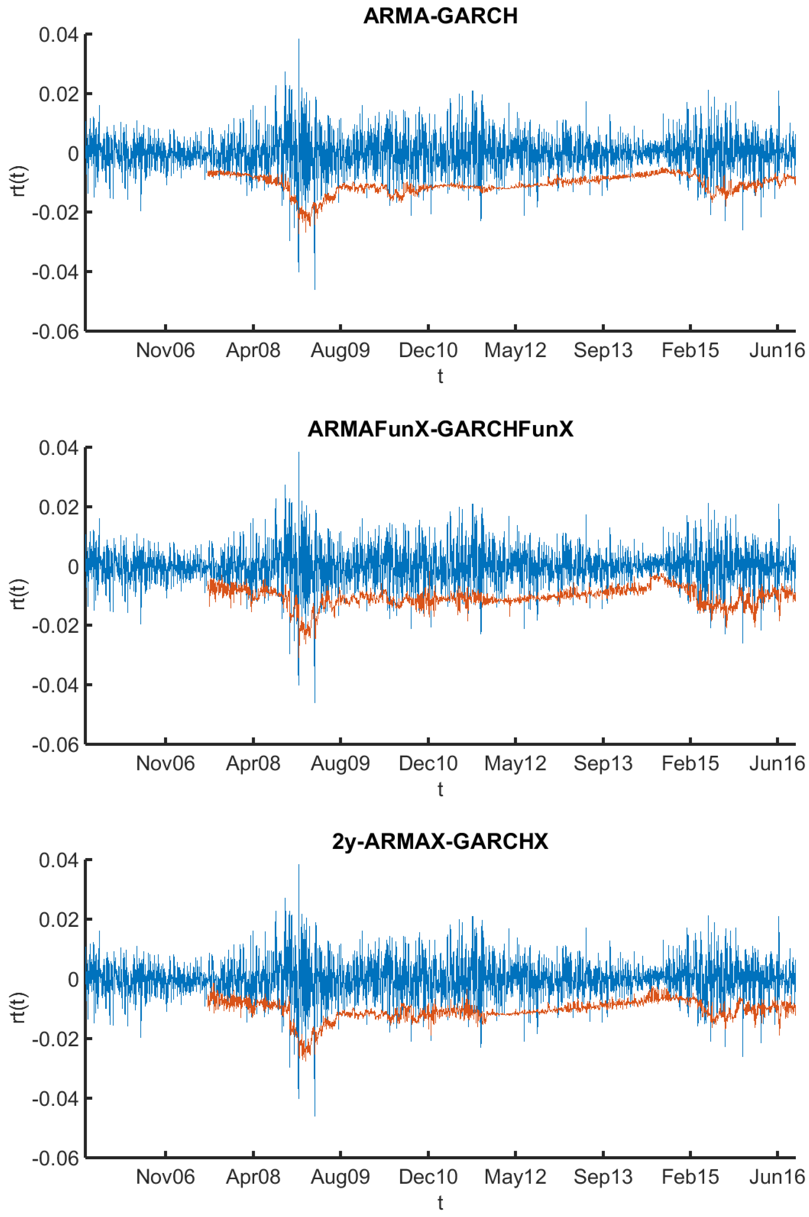
4.1. Model Fit

We start by considering the model fit of our new ARMAFunX-GARCHFunX setup taking a classical ARMA-GARCH and an ARMAX-GARCHX with just the 2y-yield differential as the exogenous variable and Gaussian errors for both as benchmarks.

Table 1. Parameter estimates, bootstrapped means and bootstrapped 95%-confidence intervals using 10,000 simulated paths of length 2903.

	ARMA-GARCH			ARMAFunX-GARCHFunX			2y-ARMAX-GARCHX
Parameters	Estimate	Mean	Confidence Interval	Estimate	Mean	Confidence Interval	Estimate	Mean	Confidence Interval
${\alpha }_0$	$1.12\times {10}^{-5}$	$3.34\times {10}^{-5}$	$[-5.12\times {10}^{-4},6.06\times {10}^{-4}]$	$1.21\times {10}^{-5}$	$1.59\times {10}^{-5}$	$[-1.71\times {10}^{-4},2.22\times {10}^{-4}]$	$2.02\times {10}^{-5}$	$2.08\times {10}^{-5}$	$[-3.24\times {10}^{-4},3.65\times {10}^{-4}]$
$\alpha$	$6.09\times {10}^{-1}$	$1.51\times {10}^{-3}$	$[-9.37\times {10}^{-1},9.41\times {10}^{-1}]$	$5.82\times {10}^{-1}$	$5.10\times {10}^{-1}$	$[-1.99\times {10}^{-1},8.34\times {10}^{-1}]$	$4.05\times {10}^{-1}$	$4.03\times {10}^{-1}$	$[3.09\times {10}^{-1},4.91\times {10}^{-1}]$
$\beta$	$-6.09\times {10}^{-1}$	$-1.90\times {10}^{-3}$	$[-9.43\times {10}^{-1},9.38\times {10}^{-1}]$	$-6.11\times {10}^{-1}$	$-5.41\times {10}^{-1}$	$[-8.57\times {10}^{-1},1.68\times {10}^{-1}]$	$-4.23\times {10}^{-1}$	$1.62\times {10}^{-3}$	$[-9.67\times {10}^{-2},1.02\times {10}^{-1}]$
$b_1$	−	−	−	$-1.48\times {10}^{-3}$	$-1.47\times {10}^{-3}$	$[-2.33\times {10}^{-3},-5.94\times {10}^{-4}]$	$-1.28\times {10}^{-2}$	$-1.48\times {10}^{-3}$	$[-8.93\times {10}^{-3},6.21\times {10}^{-3}]$
$b_2$	−	−	−	$-1.46\times {10}^{-4}$	$-1.80\times {10}^{-4}$	$[-1.91\times {10}^{-3},1.48\times {10}^{-3}]$	−	−	−
$b_3$	−	−	−	$6.80\times {10}^{-4}$	$6.77\times {10}^{-4}$	$[-1.91\times {10}^{-3},3.27\times {10}^{-3}]$	−	−	−
$\omega$	$-2.10\times {10}^{-2}$	$-3.21\times {10}^{-2}$	$[-7.81\times {10}^{-2},-6.78\times {10}^{-4}]$	$-2.25\times {10}^{-2}$	$-5.12\times {10}^{-2}$	$[-8.26\times {10}^{-2},-1.40\times {10}^{-3}]$	$-4.48\times {10}^{-2}$	$-6.91\times {10}^{-2}$	$[-1.32\times {10}^{-1},-1.62\times {10}^{-2}]$
$\gamma$	$2.15\times {10}^{-2}$	$2.11\times {10}^{-2}$	$[1.54\times {10}^{-2},2.69\times {10}^{-2}]$	$2.05\times {10}^{-2}$	$1.86\times {10}^{-2}$	$[1.27\times {10}^{-2},2.46\times {10}^{-2}]$	$2.22\times {10}^{-2}$	$1.97\times {10}^{-2}$	$[1.38\times {10}^{-2},2.60\times {10}^{-2}]$
$\delta$	$9.73\times {10}^{-1}$	$9.72\times {10}^{-1}$	$[9.64\times {10}^{-1},9.80\times {10}^{-1}]$	$9.74\times {10}^{-1}$	$9.73\times {10}^{-1}$	$[9.66\times {10}^{-1},9.83\times {10}^{-1}]$	$9.70\times {10}^{-1}$	$9.70\times {10}^{-1}$	$[9.60\times {10}^{-1},9.81\times {10}^{-1}]$
$c_1$	−	−	−	$6.50\times {10}^{-2}$	$6.61\times {10}^{-2}$	$[2.85\times {10}^{-2},1.06\times {10}^{-1}]$	$-2.06\times {10}^{-1}$	$-2.05\times {10}^{-1}$	$[-5.48\times {10}^{-1},1.22\times {10}^{-1}]$
$c_2$	−	−	−	$-8.93\times {10}^{-2}$	$-9.12\times {10}^{-2}$	$[-1.60\times {10}^{-1},-2.38\times {10}^{-2}]$	−	−	−
$c_3$	−	−	−	$1.07\times {10}^{-1}$	$1.01\times {10}^{-1}$	$[-5.41\times {10}^{-2},2.56\times {10}^{-1}]$	−	−	−

shows the parameter estimates for all three models. To assess the models’ convergence, which was discussed in Section 3.2, we carried out a simulation study; For each setup, we simulated 10,000 paths of length 2903 using the initially estimated parameters and re-estimated these based on each path. Table 1 now additionally contains the means of these bootstrapped estimates and 95%-confidence intervals.

Considering the latter, we found that apparently the 2y-yield differential has no significant effect on the ARMAX-GARCHX setup, contradicting the industry’s common belief.3 However, for the functional setup, the situation looks much brighter even though there are parts without significance, as well. To reduce dimensionality and ensure the models’ stabilities, we set all non-significant parameters (expect the intercepts) to zero and re-estimated all setups, which led to

Table 2. Parameter estimates, bootstrapped means and bootstrapped 95%-confidence intervals using 10,000 simulated paths of length 2903 restricting the models from Table 1 to significant parameters only.

	ARMA-GARCH			ARMAFunX-GARCHFunX			2y-ARMAX-GARCHX
Parameters	Estimate	Mean	Confidence Interval	Estimate	Mean	Confidence Interval	Estimate	Mean	Confidence Interval
${\alpha }_0$	$3.18\times {10}^{-5}$	$3.56\times {10}^{-5}$	$[-4.44\times {10}^{-4},5.05\times {10}^{-4}]$	$3.19\times {10}^{-5}$	$3.27\times {10}^{-5}$	$[-3.50\times {10}^{-4},4.06\times {10}^{-4}]$	$3.11\times {10}^{-5}$	$3.04\times {10}^{-5}$	$[-3.97\times {10}^{-4},4.55\times {10}^{-4}]$
$\alpha$	−	−	−	−	−	−	$5.98\times {10}^{-3}$	$5.68\times {10}^{-3}$	$[-3.51\times {10}^{-2},4.50\times {10}^{-2}]$
$\beta$	−	−	−	−	−	−	−	−	−
$b_1$	−	−	−	$-1.21\times {10}^{-3}$	$-1.21\times {10}^{-3}$	$[-2.06\times {10}^{-3},-3.63\times {10}^{-4}]$	−	−	−
$b_2$	−	−	−	−	−	−	−	−	−
$b_3$	−	−	−	−	−	−	−	−	−
$\omega$	$-1.78\times {10}^{-2}$	$-2.41\times {10}^{-2}$	$[-7.00\times {10}^{-2},5.07\times {10}^{-3}]$	$-2.21\times {10}^{-2}$	$-3.04\times {10}^{-2}$	$[-8.08\times {10}^{-2},1.33\times {10}^{-3}]$	$-2.37\times {10}^{-2}$	$-3.60\times {10}^{-2}$	$[-8.24\times {10}^{-2},-2.31\times {10}^{-3}]$
$\gamma$	$2.43\times {10}^{-2}$	$2.57\times {10}^{-2}$	$[1.93\times {10}^{-2},3.24\times {10}^{-2}]$	$2.33\times {10}^{-2}$	$2.37\times {10}^{-2}$	$[1.73\times {10}^{-2},3.05\times {10}^{-2}]$	$2.11\times {10}^{-2}$	$2.06\times {10}^{-2}$	$[1.51\times {10}^{-2},2.65\times {10}^{-2}]$
$\delta$	$9.70\times {10}^{-1}$	$9.68\times {10}^{-1}$	$[9.58\times {10}^{-1},9.76\times {10}^{-1}]$	$9.71\times {10}^{-1}$	$9.70\times {10}^{-1}$	$[9.60\times {10}^{-1},9.78\times {10}^{-1}]$	$9.73\times {10}^{-1}$	$9.72\times {10}^{-1}$	$[9.64\times {10}^{-1},9.81\times {10}^{-1}]$
$c_1$	−	−	−	$5.47\times {10}^{-2}$	$5.37\times {10}^{-2}$	$[1.36\times {10}^{-2},9.31\times {10}^{-2}]$	−	−	−
$c_2$	−	−	−	$-1.16\times {10}^{-1}$	$-1.17\times {10}^{-1}$	$[-1.84\times {10}^{-1},-4.77\times {10}^{-2}]$	−	−	−
$c_3$	−	−	−	−	−	−	−	−	−

.4 By evaluating the models’ in-sample fit via AIC and BIC (

Table 3. logL, AIC and BIC, corresponding to the full models from Table 1.

Model	logL	AIC	BIC
ARMA-GARCH	10,826	−21,639	−21,604
ARMAFunX-GARCHFunX	10,868	−21,711	−21,640
2y-ARMAX-GARCHX	10,841	−21,666	−21,619

), it can directly be seen that the ARMAFunX-GARCHFunX exhibited the lowest AIC and BIC, i.e., fit the data best, with the 2y-ARMAX-GARCHX coming in second. Restricting the models to significant parameters only (

Table 4. logL, AIC and BIC, corresponding to the restricted models from Table 2.

Model	logL	AIC	BIC
ARMA-GARCH	10,8325	−21,656	−21,632
ARMAFunX-GARCHFunX	10,863	−21,712	−21,670
2y-ARMAX-GARCHX	10,829	−21,649	−21,619

) improved the fit for all models, but the 2y-ARMAX-GARCHX.

4.2. VaR Backtesting

In the next step, we wanted to assess the out-of-sample-fit of our setups and investigate further whether the yield curve differential can effectively improve risk forecasts for the EURUSD exchange rate. For computational simplicity and to ensure better comparability, we shall from now on work with the full models depicted in Table 1 to avoid identifying the best model for each window separately. In particular, we shall apply the well-known methods from Christoffersen (1998).6

Now, using a 500-day rolling window, we estimate the full models from Table 1 and calculate one-day ahead VaR forecasts via:

$${\widehat{\mathrm{VaR}}}_{t|t-1}\left(p\right)={\widehat{\mu }}_t+{\mathsf{\Phi }}^{-1}\left(p\right){\widehat{\sigma }}_t$$

for $1-p\in \{99\%,97.5\%,95\%\}$, the standard normal cumulative distribution function $\mathsf{\Phi }$ and with ${\widehat{\mu }}_t$ being the estimated mean obtained from the ARMA parts and ${\widehat{\sigma }}_t$ the volatility estimated via GARCH, respectively.

This leaves us with 2404 VaR forecasts for each model.

Table 5. VaR prediction performance with a window size of 500 days for ARMA-GARCH, ARMAFunX-GARCHFunX and 2y-ARMAX-GARCHX for $1-p\in \{99\%,97.5\%,95\%\}$. Bold numbers denote significant values at the $5\%$-level.

Model	p	% Viol.	${\mathbf{LR}}_{\mathbf{uc}}$	${\mathbf{LR}}_{\mathbf{ind}}$	${\mathbf{LR}}_{\mathbf{cc}}$
ARMA-GARCH	$1\%$	$1.46\times {10}^{-02}$	$\mathbf{4.42}\times {\mathbf{10}}^{\mathbf{00}}$	$1.03\times {10}^{00}$	$5.49\times {10}^{00}$
	$2.5\%$	$2.79\times {10}^{-02}$	$7.84\times {10}^{-01}$	$6.19\times {10}^{-01}$	$1.46\times {10}^{00}$
	$5\%$	$5.20\times {10}^{-02}$	$1.99\times {10}^{-01}$	$4.15\times {10}^{-02}$	$3.48\times {10}^{-01}$
ARMAFunX-	$1\%$	$1.50\times {10}^{-02}$	$\mathbf{5.21}\times {\mathbf{10}}^{\mathbf{00}}$	$1.10\times {10}^{00}$	$\mathbf{6.34}\times {\mathbf{10}}^{\mathbf{00}}$
GARCHFunX	$2.5\%$	$2.83\times {10}^{-02}$	$1.02\times {10}^{00}$	$\mathbf{3.96}\times {\mathbf{10}}^{\mathbf{00}}$	$5.04\times {10}^{00}$
	$5\%$	$5.07\times {10}^{-02}$	$2.82\times {10}^{-02}$	$\mathbf{7.21}\times {\mathbf{10}}^{\mathbf{00}}$	$\mathbf{7.34}\times {\mathbf{10}}^{\mathbf{00}}$
2y-ARMAX-GARCHX	$1\%$	$1.58\times {10}^{-02}$	$\mathbf{6.96}\times {\mathbf{10}}^{\mathbf{00}}$	$1.22\times {10}^{00}$	$\mathbf{8.21}\times {\mathbf{10}}^{\mathbf{00}}$
	$2.5\%$	$2.83\times {10}^{-02}$	$1.02\times {10}^{00}$	$5.66\times {10}^{-01}$	$1.65\times {10}^{00}$
	$5\%$	$5.20\times {10}^{-02}$	$1.99\times {10}^{-01}$	$1.23\times {10}^{00}$	$1.53\times {10}^{00}$

depicts the percentage of violations and the likelihood ratio tests for unconditional coverage, independence and conditional coverage as proposed by Christoffersen (1998). Figure 4 shows the standard 5%-VaR forecasts compared to the actual log-returns for all three models.

In the following, we briefly recall the basic idea of these statistics.

• Firstly, we have the unconditional coverage (uc) test, which assumes the independence of the violations and tests the hypothesis that the empirical percentage of violations is equal to the expected p.
• The independence test (ind) checks for the independence of violations or detects clustering, respectively.
• Finally, there is the conditional coverage (cc) test that compares the empirical percentage of violations and the expected percentage as the unconditional coverage test does, but considers a possible dependence structure of the violations. We may treat it as a combination of the former two tests.
• The statistics ${\mathrm{LR}}_{\mathrm{uc}}$ and ${\mathrm{LR}}_{\mathrm{ind}}$ for the uc test and the ind test are ${\chi }^2$-distributed with one degree of freedom, whereas the ${\mathrm{LR}}_{\mathrm{cc}}$, the one for the cc test, is ${\chi }^2$-distributed with two degrees of freedom.

Summing things up, Table 5 does not show an improvement in using the yield curve data, apart from the $5\%$-VaR, where our functional model delivers a better unconditional coverage statistics than the benchmark, which in this case means that the expected and the empirical numbers of violations are very close. Even then, the ARMAXFunX-GARCHFunX exhibits a clustering of violations and therefore a worse independence test and conditional coverage test statistics.

As mentioned before, the ${\mathrm{LR}}_{\mathrm{cc}}$ can be seen as a combination of the ${\mathrm{LR}}_{\mathrm{uc}}$ and the ${\mathrm{LR}}_{\mathrm{ind}}.$ Therefore, in most cases, ${\mathrm{LR}}_{\mathrm{cc}}$ had a high value whenever ${\mathrm{LR}}_{\mathrm{uc}}$ had one as well. The exceptions were the cases in which the independence test statistics was unusually high. High values of ${\mathrm{LR}}_{\mathrm{ind}}$ hinted towards a clustering of violations. This phenomenon can especially be observed at the 5%-VaR from the ARMAFunX-GARCHFunX, where the unconditional coverage test statistics was rather small and well below the significance level, but because of the clustering, we had a significant ${\mathrm{LR}}_{\mathrm{cc}}.$

Finally, we want to note that we carried out robustness checks regarding the actual number of principal components for the functional setup. We experienced an increase of clustering of violations while adding more principal components to our model, with the change from two to three principal components having the biggest impact on the ${\mathrm{LR}}_{\mathrm{ind}}$. Note that, since ${\mathrm{LR}}_{\mathrm{cc}}$ can be seen as a combination of ${\mathrm{LR}}_{\mathrm{uc}}$ and ${\mathrm{LR}}_{\mathrm{ind}}$, this influenced the conditional coverage, as well. This phenomenon appeared to be capped at three principal components, which was observable in particular for the 5%-VaR. Interestingly, using two principal components instead of just one achieved worse results for all $p\in \{1\%,2.5\%,5\%\}.$ The performances of the models with three and four principal components did not differ much, apart from a noticeably smaller ${\mathrm{LR}}_{\mathrm{ind}}$ for the 2.5%-VaR. Finally, we want to point out that our model, which used three principal components, had the smallest ${\mathrm{LR}}_{\mathrm{uc}}$ for the 5%-VaR compared to incorporating 1, 2 or 4 principal components.

Consequently, we can further confirm that employing yield curve information seemed to be able to improve VaR forecasting for FX rates in some situations.

5. Discussion

This paper introduces a new approach in implementing macroeconomic data, in particular yield curve information in FX rate models. As we have shown in detail in Section 1, the general idea of such an approach can be found throughout the literature. However, according to the efficient market hypothesis, interest rate differentials cannot be used for forecasting FX rates in a sensible fashion. We do not argue this and will not delve into a discussion about the failure of the uncovered interest rate parity. Therefore, we utilize our ARMAXFunX-GARCHFunX for forecasting risk, in particular the VaR of the EURUSD rate.

The way our model sticks out and improves on older approaches is the use of functional principal component analysis to implement the whole shape of the yield curve as an exogenous variable.

Applying principal components in this way has been done in a similar fashion before. We refer to Fuest and Mittnik (2015), who presented the GARCH-FunXL model and used the functional approach to model asset price volatility. The information contained in the stock exchange’s limit order book is extracted by means of functional principal component analysis, and its impact on asset price volatility is analyzed. The work in Fuest and Mittnik (2015) reported an improved forecasting performance compared to models without liquidity impact.

We extend their GARCH-FunXL setup by allowing for an additional ARMAXFunX part and invoke this more generalized setup to forecast the VaR of FX rates.

The data used for our yield curves consist of overnight index swaps on the EONIA and the EONIA for shortest maturity and the US treasury yields, with the Fed Funds rate for the shortest maturity. Interpolation and taking differentials7 gives us the data matrix of the yield curve differentials used for our analysis. We transform this matrix of yield differentials into functional data, which means that we get a stochastic process ${\left(x_t\right)}_{t\in \mathcal{T}},$ where each $x_t$ maps maturities to yields. The theory for functional principal component analysis, which is needed to understand the basic idea of the model, is introduced in Section 3.

Although our functional model exhibits clustering of violations, we experienced a smaller unconditional coverage statistics for the 5%-VaR, which means that the estimated number of violations was very close to the expected number. Summing up, we confirm that employing yield curve information is able to improve VaR forecasting for FX rates in some situations. This established connection between yield curve data and FX risk goes with the findings in the literature: Dominguez (1998) modeled FX rate volatility via a GARCH(1,1) setup that incorporated, among other variables, overnight index rate differentials corresponding to the FX rates in question as exogenous variables, an approach similar to ours, and found the interest rate differentials to have a significant impact on FX rate volatility. We further mention Neely (1999), who analyzed the connection of realignment and conditional volatility in target zone exchange rate systems via a jump-diffusion GARCH model, where they used interest rate differentials and a proxy for the domestic yield curve to model a country-specific realignment probability or jump probability. Letting the jump-intensity vary with dependence on the interest rates in this way allows the model to detect realignments before they happen. With this setup, the precision of forecasts can be improved. As for a connection between macroeconomic volatility and FX rate volatility, we recall Morana (2009). He used principal component analysis to extract the relevant factors for macroeconomic volatility and FX rate volatility, respectively, and showed that there is an influence from macro to FX, especially for the long-term. Among other macro variables, he used short-term interest rates, in particular three-month government bills. An improvement in out-of-sample forecasting performance, using this setup, was reported. This result supports our findings, since we confirm that the yield curve information contains valuable information for forecasting FX rate volatility, which is confirmed by Dunis and Huang (2002), as mentioned in the Introduction. Finally, we mention Bauwens and Sucarrat (2010), who compared the forecasting performance of several models of exchange rate volatility in the GETS (general-to-specific) approach and did find evidence of an improvement by the inclusion of macro variables, such as interest rates.

Summing up, this points towards an influence of macroeconomic or, in particular, yield curve data on modeling FX risk. One property that most basic models of FX rates or FX rate volatility share though is that an increase in the exogenous information used always leads to a higher number of variables. Implementing the exogenous data as functional data and using the power of functional principal component analysis allow us to contain almost all of the information contained within any dataset by about three principal components, no matter the size of the matrix.

Coming to a conclusion, we find that the ARMAXFunX-GARCHFunX enriches the family of ARMAX-GARCHX models by allowing the implementation of the information contained in a data matrix via its principal components or its principal component scores, respectively, no matter how big it is or, in our case, how many maturities we want to implement, a feature that is, as we have seen, desirable when modeling and forecasting exchange rate volatility.

However, when it comes to actually using our newly-proposed forecasting setup, we see just some minor improvements on a classical ARMAX-GARCHX benchmark containing just the 2y-yield as the exogenous variable for, e.g., the 5%-VaR unconditional coverage, but are not able to detect a more general advantage of the functional setup. However, considering different lags and (fat-tailed) error distributions might be a fruitful start for future research in this area and might justify the usage of, for example, more maturities, as discussed above.

Furthermore, we want to stress the fact that the data in the present study are based on first-step estimates of the yield curve, which are evaluated at a rather small number of maturities. Recall the construction of our yield curves: The EUR- and the US-yield curves were equivalently constructed by using the available data as presented in Section 2 as follows. For each observation date, we used the available data points (maturities) as nodes for spline interpolation. With this procedure, a yield curve consisting of 121 maturities for EUR, as well as for the US is obtained. Taking the componentwise difference of both yield curves, which are basically data matrices, we acquire the yield curve differential of the EUR- and the US-yield curve.

Such estimates might be over-simplifying in the present context. Using the primary information on the YTMs of single securities underlying the curve estimates, additional modes of variation may be uncovered that are potentially useful to predict FX returns.

References

- Ang, Andrew, and Chen Joseph. 2010. Yield Curve Predictors of Foreign Exchange Returns. Paper presented at AFA 2011 Denver Meetings, Denver, CO, USA, January 7–9. [Google Scholar]
- Aue, Alexander, Diogo Dubart Norinho, and Siegfried Hörmann. 2015. On the prediction of stationary functional time series. Journal of the American Statistical Association 110: 378–92. [Google Scholar] [CrossRef]
- Baillie, Richard T., and Tim Bollerslev. 1991. Intra-day and inter-market volatility in foreign exchange rates. The Review of Economic Studies 58: 565–85. [Google Scholar] [CrossRef]
- Baillie, Richard T., Tim Bollerslev, and Hans Ole Mikkelsen. 1996. Fractionally integrated generalized autoregressive conditional heteroskedasticity. Journal of Econometrics 74: 3–30. [Google Scholar] [CrossRef]
- Bauwens, Luc, and Genaro Sucarrat. 2010. General-to-specific modelling of exchange rate volatility: A forecast evaluation. International Journal of Forecasting 26: 885–907. [Google Scholar] [CrossRef]
- Benavides, Guillermo, and Carlos Capistràn. 2012. Forecasting exchange rate volatility: The superior performance of conditional combinations of time series and option implied forecasts. Journal of Empirical Finance 19: 627–39. [Google Scholar] [CrossRef]
- Bjørnland, Hilde C., and Håvard Hungnes. 2006. The importance of interest rates for forecasting the exchange rate. Journal of Forecasting 25: 209–21. [Google Scholar] [CrossRef]
- Bosq, Denis. 2000. Linear Processes in Function Spaces: Theory and Applications. Berlin: Springer. [Google Scholar]
- Brockhaus, Sarah, Andreas Fuest, Andreas Mayr, and Sonja Greven. 2017. Signal regression models for location, scale and shape with an application to stock returns. Journal of the Royal Statistical Society/Series C (Applied Statistics) 67: 665–86. [Google Scholar] [CrossRef]
- Campbell, John Y., and Richard H. Clarida. 1987. The dollar and real interest rates. Carnegie-Rochester Conference Series on Public Policy 27: 103–39. [Google Scholar] [CrossRef]
- Chen, Yu-chin, and Kwok Ping Tsang. 2013. What does the yield curve tell us about exchange rate predictability? Review of Economics and Statistics 95: 185–205. [Google Scholar] [CrossRef]
- Chinn, Menzie D., and Richard A. Meese. 1995. Banking on currency forecasts: How predictable is change in money? Journal of International Economics 38: 161–78. [Google Scholar] [CrossRef]
- Christiansen, Charlotte, Maik Schmeling, and Andreas Schrimpf. 2012. A comprehensive look at financial volatility prediction by economic variables. Journal of Applied Econometrics 27: 956–77. [Google Scholar] [CrossRef]
- Christoffersen, Peter F. 1998. Evaluating interval forecasts. International Economic Review 39: 841–62. [Google Scholar] [CrossRef]
- Coughlin, Cletus C., and Kees Koedijk. 1990. What do we know about the long-run real exchange rate? Federal Reserve Bank of St. Louis Review 72. [Google Scholar] [CrossRef]
- Diebold, Francis X., and Canlin Li. 2006. Forecasting the term structure of government bond yields. Journal of Econometrics 130: 337–64. [Google Scholar] [CrossRef]
- Dominguez, Kathryn M. 1998. Central bank intervention and exchange rate volatility. Journal of International Money and Finance 17: 161–90. [Google Scholar] [CrossRef]
- Dunis, Christian L., and Xuehuan Huang. 2002. Forecasting and trading currency volatility: An application of recurrent neural regression and model combination. Journal of Forecasting 21: 317–54. [Google Scholar] [CrossRef]
- Edison, Hali J., and B. Dianne Pauls. 1993. A re-assessment of the relationship between real exchange rates and real interest rates: 1974–1990. Journal of Monetary Economics 31: 165–87. [Google Scholar] [CrossRef]
- European Banking Federation (FBE). 2008. EONIA Swap Index: The Derivatives Market Reference Rate for the Euro. Brussels: European Banking Federation. [Google Scholar]
- Fama, Eugenel. 1970. Efficient capital markets: A review of theory and empirical work. The Journal of Finance 25: 383–417. [Google Scholar] [CrossRef]
- Filipović, Damir, and Anders B. Trolle. 2013. The term structure of interbank risk. Journal of Financial Economics 109: 707–33. [Google Scholar] [CrossRef]
- Francq, Christian, Olivier Wintenberger, and Jean-Michael Zakoïan. 2013. GARCH models without positivity constraints: Exponential or log GARCH? Journal of Econometrics 177: 34–46. [Google Scholar] [CrossRef]
- Frankel, Jeffrey A., and Andrew K. Rose. 1995. Empirical research on nominal exchange rates. In Handbook of International Economics. Edited by G. M. Grossman and Kenneth Rogoff. Amsterdam: North Holland Publishing Company, vol. 3, pp. 1689–729. [Google Scholar]
- Fuest, Andreas, and Stefan Mittnik. 2015. Modeling Liquidity Impact on Volatility: A GARCH-FunXL Approach. Available online: http://dx.doi.org/10.2139/ssrn.3038947 (accessed on 16 August 2018).
- Grisse, Christian, and Thomas Nitschka. 2015. On financial risk and the safe haven characteristics of swiss franc exchange rates. Journal of Empirical Finance 32: 153–64. [Google Scholar] [CrossRef]
- Han, Heejon. 2015. Asymptotic properties of GARCH-X processes. Journal of Financial Econometrics 13: 188–221. [Google Scholar] [CrossRef]
- Han, Heejon, and Dennis Kristensen. 2014. Asymptotic theory for the QMLE in GARCH-X models with stationary and nonstationary covariates. Journal of Business & Economic Statistics 32: 416–29. [Google Scholar]
- Hannan, Edward J., William T. M. Dunsmuir, and Manfred Deistler. 1980. Estimation of vector ARMAX models. Journal of Multivariate Analysis 10: 275–95. [Google Scholar] [CrossRef]
- Hansen, Peter Reinhard, Zhuo Huang, and Howard Howan Shek. 2012. Realized GARCH: A joint model for returns and realized measures of volatility. Journal of Applied Econometrics 27: 877–906. [Google Scholar] [CrossRef]
- Hörmann, Siegfried, Lajos Horváth, and Ron Reeder. 2013. A functional version of the ARCH model. Econometric Theory 29: 267–88. [Google Scholar] [CrossRef]
- Hörmann, Siegfried, and Piotr Kokoszka. 2010. Weakly dependent functional data. The Annals of Statistics 38: 1845–84. [Google Scholar] [CrossRef]
- Hörmann, Siegfried, and Piotr Kokoszka. 2012. Functional time series. In Handbook of Statistics: Time Series Analysis: Methods and Applications, 1st ed. Edited by Tata Subba Rao, Suhasini Subba Rao and C. R. Rao. Amsterdam: North Holland Publishing Company, vol. 30, p. 157. [Google Scholar]
- Hull, John, and Alan White. 1998. Value at risk when daily changes in market variables are not normally distributed. Journal of Derivatives 5: 9–19. [Google Scholar] [CrossRef]
- Hull, John, and Alan White. 2012. Libor VS OIS: The derivatives discounting dilemma. Journal of Investment Management 11: 14–27. [Google Scholar] [CrossRef]
- Hyndman, Rob J., and Han Lin Shang. 2009. Forecasting functional time series. Journal of the Korean Statistical Society 38: 199–211. [Google Scholar] [CrossRef]
- Ichiue, Hibiki, and Kentaro Koyama. 2011. Regime switches in exchange rate volatility and uncovered interest parity. Journal of International Money and Finance 30: 1436–50. [Google Scholar] [CrossRef]
- Klepsch, Johannes, Claudia Klüppelberg, and Taoran Wei. 2017. Prediction of functional ARMA processes with an application to traffic data. Econometrics and Statistics 1: 128–49. [Google Scholar] [CrossRef]
- Kočenda, Evžen, and Tigran Poghosyan. 2009. Macroeconomic sources of foreign exchange risk in new EU members. Journal of Banking & Finance 33: 2164–73. [Google Scholar]
- Kowal, Daniel R., David S. Matteson, and David Ruppert. 2017. A Bayesian multivariate functional dynamic linear model. Journal of the American Statistical Association 112: 733–44. [Google Scholar] [CrossRef]
- Kowal, Daniel R., David S. Matteson, and David Ruppert. 2017. Functional autoregression for sparsely sampled data. Journal of Business & Economic Statistics. [Google Scholar] [CrossRef]
- Kuester, Keith, Stefan Mittnik, and Marc S. Paolella. 2006. Value-at-risk prediction: A comparison of alternative strategies. Journal of Financial Econometrics 4: 53–89. [Google Scholar] [CrossRef]
- Markiewicz, Agnieszka. 2012. Model uncertainty and exchange rate volatility. International Economic Review 53: 815–44. [Google Scholar] [CrossRef]
- Meese, Richard, and Kenneth Rogoff. 1983. Empirical exchange rate models of the seventies-Do they fit out of sample? Journal of International Economics 14: 3–24. [Google Scholar] [CrossRef]
- Meese, Richard, and Kenneth Rogoff. 1988. Was it real? The exchange rate-interest differential relation over the modern floating-rate period. The Journal of Finance 43: 933–48. [Google Scholar] [CrossRef]
- Mittnik, Stefan, and Marc S. Paolella. 2000. Conditional density and value-at-risk prediction of Asian currency exchange rates. Journal of Forecasting 19: 313–33. [Google Scholar] [CrossRef]
- Morana, Claudio. 2009. On the macroeconomic causes of exchange rate volatility. International Journal of Forecasting 25: 328–50. [Google Scholar] [CrossRef]
- Neely, Christopher J. 1999. Target zones and conditional volatility: The role of realignments. Journal of Empirical Finance 6: 177–92. [Google Scholar] [CrossRef]
- Ramsay, James O. 2014. FDA Toolbox. Available online: http://www.psych.mcgill.ca/misc/fda/index.html (accessed on 16 August 2018).
- Ramsay, James O., and Bernard W. Silverman. 2005. Functional Data Analysis. New York: Springer. [Google Scholar]
- Sheppard, Kevin. 2013. MFE Toolbox. Available online: https://www.kevinsheppard.com/MFE_Toolbox (accessed on 16 August 2018).
- Sucarrat, Genaro, Steffen Grønneberg, and Alvaro Escribano. 2016. Estimation and inference in univariate and multivariate log-GARCH-x models when the conditional density is unknown. Computational Statistics & Data Analysis 100: 582–94. [Google Scholar]
- Vilasuso, Jon. 2002. Forecasting exchange rate volatility. Economic Letters 76: 59–64. [Google Scholar] [CrossRef]
- West, Kenneth D., Hali J. Edison, and Dongchul Cho. 1993. A utility-based comparison of some models of exchange rate volatility. Journal of International Economics 35: 23–45. [Google Scholar] [CrossRef]
- Wied, Dominik, George N.F. Weiß, and Daniel Ziggel. 2016. Evaluating value-at-risk forecasts: A new set of multivariate backtests. Journal of Banking & Finance 72: 121–32. [Google Scholar]
- Ziggel, Daniel, Tobias Berens, Geroge N. F. Weiß, and Dominis Wied. 2014. A new set of improved value-at-risk backtests. Journal of Banking & Finance 48: 29–41. [Google Scholar]