Bayesian Adjustment for Insurance Misrepresentation in Heavy-Tailed Loss Regression

Abstract

In this paper, we study the problem of misrepresentation under heavy-tailed regression models with the presence of both misrepresented and correctly-measured risk factors. Misrepresentation is a type of fraud when a policy applicant gives a false statement on a risk factor that determines the insurance premium. Under the regression context, we introduce heavy-tailed misrepresentation models based on the lognormal, Weibull and Pareto distributions. The proposed models allow insurance modelers to identify risk characteristics associated with the misrepresentation risk, by imposing a latent logit model on the prevalence of misrepresentation. We prove the theoretical identifiability and implement the models using Bayesian Markov chain Monte Carlo techniques. The model performance is evaluated through both simulated data and real data from the Medical Panel Expenditure Survey. The simulation study confirms the consistency of the Bayesian estimators in large samples, whereas the case study demonstrates the necessity of the proposed models for real applications when the losses exhibit heavy-tailed features.

1. Introduction

In both property and casualty and general insurance, regression models are widely used for rate making purposes (see, e.g., Bermúdez and Karlis (2015); Hua (2015); Klein et al. (2014)). Among them, generalized linear models (GLMs) have become popular choices (see, e.g., Brockman andWright (1992); David (2015); Haberman and Renshaw (1996)), probably owing to the well-developed theories and algorithms for inference based on maximum likelihood estimation (MLE). For example, the Poisson and negative binomial regression models are popular for loss frequency modeling, while the gamma model is a popular loss severity model recognized by the insurance industry.

In real applications, however, loss data often exhibit heavy-tailed features that cannot be captured by the exponential family of distributions under GLMs. As a result, statistical and probability theories for the heavy-tail phenomena have become popular research topics in the past decade (see, e.g., Hao and Tang (2012); Qi (2010); Yang et al. (2018)). For statistical inference purposes, earlier papers such as Scollnik (2001 2002 2015) proposed to use Bayesian inference based on Markov chain Monte Carlo (MCMC) simulations, whereas books and papers including Peng and Qi (2017); Qi (2010) promoted the use of frequentist counter-parts. For loss severity outcomes, Scollnik (2001, 2002) illustrated the use of Bayesian inference using Gibbs sampling (BUGS) for implementing MCMC algorithms for heavy-tailed models from the lognormal, Pareto and and Weibull distributions.

For the problem of insurance misrepresentation, Xia and Gustafson (2016) is the first paper that studied the model identification and implementation when concerning the association between a response and a binary risk factor subject to misrepresentation. The paper used the term unidirectional misclassification from Gustafson (2014) for the type of measurement such as misrepresentation where the error occurs only in one direction that favors the respondent. Later papers including Sun et al. (2017); Xia and Gustafson (2018) inherited the terminology and extended the work to the two cases where the variable of concern is an ordinal covariate and a binary response. Most of the earlier papers concerned the model identifiability corresponding to the existence of a unique maximum in the likelihood function with respect to the observed variables. For all the earlier papers except for Gustafson (2014); Hahn et al. (2016), the models possessed the identifiability, which enables us to perform statistical inference on all the model parameters without prior knowledge on the severity of misrepresentation. In the most recent paper concerning the problem of misrepresentation (Xia et al. 2018), the model from Xia and Gustafson (2016) was expanded for the purpose of predictive analytics on the misrepresentation risk, while including multiple risk factors with some of them subject to misrepresentation.

In this paper, we extend the misrepresentation models from Xia et al. (2018) to the case where the association between the claim severity and risk factors is modeled through heavy-tailed regression. Based on the lognormal, Pareto and Weibull distributions, we establish the misrepresentation models for heavy-tailed loss outcomes. The models encompass both misrepresented and correctly-measured risk factors in the heavy-tailed regression, with the adjustment of misrepresentation undertaken through latent logit regression on the prevalence of misrepresentation. The latent regression allows insurance companies to assess the effect of other risk factors on the misrepresentation risk. From the theoretical perspective, we prove the identifiability of the heavy-tailed misrepresentation models based on the specific mixture regression structures obtained earlier for the conditional distribution of the observed variables (Xia et al. 2018), confirming that consistent estimation is guaranteed for the model parameters. We implement the models in BUGS (Scollnik 2001; Xia et al. 2018) and perform simulation studies to evaluate the performance of models under finite samples. From the simulation studies, ignoring the misrepresentation in the naive analysis gives rise to bias in the estimated risk effect(s), whereas the proposed models correct for the bias based on learning from the mixture structures. Furthermore, the simulation studies illustrate the convergence of the estimators toward their true values at the rate of $\sqrt{1/n}$ in large samples, for all the parameters in the proposed models including those concerning the regression coefficients and the prevalence of misrepresentation. This confirms the theoretical results on the model identifiability and the classical statistical theories on the speed of convergence for Bayesian estimators. Using the 2013 Medical Expenditure Panel Survey (MEPS) data, we perform a model comparison based on the deviance information criterion (DIC) and select the Pareto misrepresentation model as the model with the optimal goodness of fit. The case study demonstrates that the heavy-tailed models can be useful for real applications where the losses often exhibit heavy-tailed features.

The rest of the paper is organized as follows. In Section 2, we review the misrepresentation models from Xia et al. (2018) and extend them to the heavy-tailed regression context. In Section 3, we prove the theoretical identifiability of the misrepresentation models for the Weibull, lognormal and Pareto distribution families. Section 4 presents simulation studies for the lognormal, Pareto and Weibull models. In Section 5, a model comparison is performed using the 2013 MEPS data. Section 6 concludes the paper.

2. Heavy-Tailed Loss Models under Misrepresentation

In this section, we will extend the predictive models from Xia et al. (2018) to the context of heavy-tailed loss regression.

2.1. The Misrepresentation Problem

We first use notation from Xia and Gustafson (2016) to formulate the problem of misrepresentation with a binary risk factor. Let V and $V^{\ast }$ denote the true binary risk status and the observed status, respectively. We assume that misrepresentation may occur with a positive probability, when the individual has a positive risk status. In particular, we can write the conditional probabilities as:

$$\begin{array}{cc}\hfill \mathrm{P}(V^{\ast }=0|V=0)& =1\hfill \\ \hfill \mathrm{P}(V^{\ast }=0|V=1)& =p,\hfill \end{array}$$

(1)

where the parameter p is referred to as the misrepresentation probability. Denoting by $\theta =\mathrm{P}(V=1)$ the true probability of a positive risk status, Xia and Gustafson (2016) derived the observed probability of a positive risk status as ${\theta }^{\ast }=\mathrm{P}(V^{\ast }=1)=\theta (1-p)$. The work in Xia et al. (2018) used the term the prevalence of misrepresentation for $q=\mathrm{P}(V=1|V^{\ast }=0)$, the percentage of reported negatives corresponding to a true positive risk status. Using Bayes’ theorem, the prevalence of misrepresentation can be obtained as $q=\theta p/[1-\theta (1-p\left)\right]$. Similarly, the misrepresentation probability can be written as $p=(1-\theta )q/\left[\theta \right(1-q\left)\right]$. That is, we can derive one conditional probability from the other, along with an estimate of the observed probability ${\theta }^{\ast }$ estimable from the samples of $V^{\ast }$. Interested readers may refer to Xia et al. (2018) for additional details.

When unadjusted, misrepresentation is expected to cause an attenuation effect in the estimated risk effect, leading to an underestimation of the risk. The underestimation of the risk effect gives rise to an increase in the premium for the low-risk applicants with a true negative status, resulting in the loss of product competitiveness in such a preferred market segment. Hence, appropriate modeling of the misrepresentation phenomena can help insurance companies better understand the severity and the financial impact of the problem, as well as providing insights into the cost-effectiveness for managing the misrepresentation risk.

2.2. Weibull Model with Additional Correctly-Measured Risk Factors

In loss regression, we are interested in modeling the mean of a response variable Y from a loss distribution, conditioning on the true risk status V and some additional risk factors $\mathbf{x}$. In Xia and Gustafson (2016); Xia et al. (2018), the authors assumed that the misrepresentation is non-differential on Y (i.e., $Y\perp V^{\ast }|V,\mathbf{x}$). This means that the outcome Y does not depend on whether the applicant misrepresents the risk factor, given the true status V and other risk factors $\mathbf{x}$. Under heavy-tailed regression, we have the same structure for the conditional distribution of the observed variables as that from Xia et al. (2018). In particular, $\left(Y\right|V^{\ast },\mathbf{x})$ has the following distributional form.

$$\begin{array}{cc}\hfill f_Y\left(y\right|V^{\ast }=1,\mathbf{x})& =f_Y\left(y\right|\mathit{\alpha },\mathit{\phi },V=1,\mathbf{x})\hfill \\ \hfill f_Y\left(y\right|V^{\ast }=0,\mathbf{x})& =q{f}_Y\left(y\right|\mathit{\alpha },\mathit{\phi },V=1,\mathbf{x})+(1-q)f_Y\left(y\right|\mathit{\alpha },\mathit{\phi },V=0,\mathbf{x}),\hfill \end{array}$$

(2)

where $f_Y\left(y\right|\mathit{\alpha },\mathit{\phi },V=v,\mathbf{x})$ denotes the conditional distribution of Y given the true status and the other risk factors, the parameter vector $\mathit{\alpha }$ contains the regression coefficients and $\mathit{\phi }$ contains any additional parameter(s) such as a shape parameter in the case of heavy-tailed models.

Given $\mathbf{x}$, the conditional distribution of $\left(Y\right|V^{\ast },\mathbf{x})$ contains two component distributions when $V^{\ast }=0$, and it is a single distribution when $V^{\ast }=1$. The mixture model in the second line of Equation (2) is called a mixture regression model when there are some additional covariates $\mathbf{x}$. Note that the parameters concerning the component $f_Y\left(y\right|V^{\ast }=1,\mathbf{x})$ can be identified using the samples with $V^{\ast }=1$. These parameters include the regression coefficients shared by both components. In heavy-tailed regression, we usually assume a common shape parameter in the two components, which also facilitates the learning of the parameters. Thus, the difference of the intercepts (i.e., the V effect) and the prevalence of misrepresentation (i.e., the mixture weight) are the only parameters that require the samples with both $V^{\ast }=0$ and $V^{\ast }=1$. The theoretical identifiability of the proposed models will be proven later in Section 3.

Under heavy-tailed regression, we first give an example Weibull misrepresentation model for the case with one risk factor V subject to misrepresentation and a correctly-measured risk factor X.

Example 1 (Weibull model).

Based on Weibull regression, we present a loss severity model for illustration purposes. Using the parametrization in BUGS for the general Weibull distribution (see, e.g., Scollnik (2002)), we can specify the loss severity model as:

$$\begin{array}{cc}\hfill \left(Y\right|V,X)& \sim Weibull(\tau ,{\lambda }_{V,X})\hfill \\ \hfill 1/{\lambda }_{V,X}& =\exp ({\alpha }_0+{\alpha }_{1}V+{\alpha }_{2}X)\hfill \\ \hfill \left(V^{\ast }\right|V,X)& \sim Bernoulli\left(\right(1-p\left)V\right),\hfill \end{array}$$

(3)

where $\tau >0$ is the shape parameter and $1/{\lambda }_{V,X}$ is proportional to the conditional mean of Y given V and X. For this example, the conditional distribution $f_Y\left(y\right|\mathit{\alpha },\mathit{\phi },V,\mathbf{x})$ in Equation (2) takes the form of the above Weibull distribution, with $\mathit{\alpha }=({\alpha }_0,{\alpha }_1,{\alpha }_2)$ and $\mathit{\phi }=\tau$.

2.3. Lognormal Model with Multiple Risk Factors Subject to Misrepresentation

In Xia et al. (2018), the authors studied another situation where there are multiple risk factors subject to misrepresentation. Let $\mathbf{v}=$($V_1$, $V_2$, ⋯, $V_J$) denote the true status of J rating factors that are subject to misrepresentation and ${\mathbf{v}}^{\ast }=$($V_1^{\ast }$, $V_2^{\ast }$, ⋯, $V_J^{\ast }$) denote the corresponding observed status for these rating factors. Here, we add additional risk factors of $\mathbf{x}$ for deriving a more general structure. Similar to Xia et al. (2018), we assume that the loss outcome Y depends on the rating factors in $\mathbf{v}$ and $\mathbf{x}$ through some regression coefficients $\mathit{\alpha }$. For the current paper, the conditional distribution of $\left(Y\right|\mathbf{v},\mathbf{x})$ can be written as $f_Y\left(y\right|\mathit{\alpha },\mathit{\phi },\mathbf{v},\mathbf{x})$. Based on the non-differential misrepresentation assumption, the conditional distribution of $\left(Y\right|{\mathbf{v}}^{\ast },\mathbf{x})$ will either be a single regression model when ${\mathbf{v}}^{\ast }=(1,1,\cdots ,1)$ or a mixture regression model with the number of components and the mean of each component determined by the observed values of the variables in ${\mathbf{v}}^{\ast }$. For example, when there are two rating factors with misrepresentation (i.e., $\mathbf{v}=$($V_1$, $V_2$)) and an additional risk factor X, we can derive the conditional distribution of observed variables, $\left(Y\right|{\mathbf{v}}^{\ast },X)$, as:

$$\begin{array}{cc}\hfill f_Y\left(y\right|V_1^{\ast }=1,V_2^{\ast }=1,X)=& f_Y\left(y\right|\mathit{\alpha },\mathit{\phi },V_1=1,V_2=1,X)\hfill \\ \hfill f_Y\left(y\right|V_1^{\ast }=0,V_2^{\ast }=1,X)=& q_1{f}_Y\left(y\right|\mathit{\alpha },\mathit{\phi },V_1=1,V_2=1,X)+(1-q_1)f_Y\left(y\right|\mathit{\alpha },\mathit{\phi },V_1=0,V_2=1,X)\hfill \\ \hfill f_Y\left(y\right|V_1^{\ast }=1,V_2^{\ast }=0,X)=& q_2{f}_Y\left(y\right|\mathit{\alpha },\mathit{\phi },V_1=1,V_2=1,X)+(1-q_2)f_Y\left(y\right|\mathit{\alpha },\mathit{\phi },V_1=1,V_2=0,X)\hfill \\ \hfill f_Y\left(y\right|V_1^{\ast }=0,V_2^{\ast }=0,X)=& q_3{f}_Y\left(y\right|\mathit{\alpha },\mathit{\phi },V_1=1,V_2=1,X)+q_4{f}_Y\left(y\right|\mathit{\alpha },\mathit{\phi },V_1=0,V_2=1,X)\hfill \\ & +q_5{f}_Y\left(y\right|\mathit{\alpha },\mathit{\phi },V_1=1,V_2=0,X)\hfill \\ & +(1-q_3-q_4-q_5)f_Y\left(y\right|\mathit{\alpha },\mathit{\phi },V_1=0,V_2=0,X),\hfill \end{array}$$

(4)

where the prevalence of misrepresentation can be defined for different scenarios: $q_1=\mathrm{P}(V_1=1,V_2=1|V_1^{\ast }=0,V_2^{\ast }=1)$, $q_2=\mathrm{P}(V_1=1,V_2=1|V_1^{\ast }=1,V_2^{\ast }=0)$, $q_3=\mathrm{P}(V_1=1,V_2=1|V_1^{\ast }=0,V_2^{\ast }=0)$, $q_4=\mathrm{P}(V_1=0,V_2=1|V_1^{\ast }=0,V_2^{\ast }=0)$ and $q_5=\mathrm{P}(V_1=1,V_2=0|V_1^{\ast }=0,V_2^{\ast }=0)$. Dependence assumptions regarding the true and observed risk factors are discussed in Xia et al. (2018).

Note that Equation (4) differs from the mixture structure in Xia et al. (2018), as the inclusion of an additional risk factor X gives rise to a mixture regression structure. Based on the mixture regression structure, we can use the lognormal distribution (see, e.g., Scollnik (2002)) to give a simplified example for the case where there are two risk factors subject to misrepresentation and an additional risk factor that is correctly measured.

Example 2 (Lognormal model).

Let Y denote the loss amount for a given policy year, ($V_1$, $V_2$) and ($V_1^{\ast }$, $V_2^{\ast }$) denote the vectors containing the true and observed risk statuses, respectively, and X denote an additional risk factor that is correctly measured. We can write the lognormal model as:

$$\begin{array}{cc}\hfill \left(Y\right|V_1,V_2,X)& \sim lognormal({\mu }_{V_1,V_2,X},{\sigma }^2)\hfill \\ \hfill {\mu }_{V_1,V_2,X}& ={\alpha }_0+{\alpha }_1{V}_1+{\alpha }_2{V}_2+{\alpha }_{3}X\hfill \\ \hfill \left(V_1^{\ast }\right|V_1,V_2,X)& \sim Bernoulli\left((1-p_1)V_1\right)\hfill \\ \hfill \left(V_2^{\ast }\right|V_1,V_2,X)& \sim Bernoulli\left((1-p_2)V_2\right),\hfill \end{array}$$

(5)

where $\exp \left({\mu }_{V_1,V_2,X}\right)$ is proportional to the conditional mean of Y given the true statuses $(V_1,V_2,X)$ and the last two lines indicate that the occurrence of misrepresentation in one risk factor is independent of that in the other. Here, the conditional distribution of $\left(Y\right|V_1^{\ast },V_2^{\ast },X)$ possesses the mixture regression structure in Equation (4), and the prevalence of misrepresentation $q_j$ is a mixture weight that can be estimated using data on $(Y,V_1^{\ast },V_2^{\ast },X)$. For this example, the conditional distribution $f_Y\left(y\right|\mathit{\alpha },\mathit{\phi },V_1,V_2,X)$ takes the form of the above lognormal distribution, with $\mathit{\alpha }=({\alpha }_0,{\alpha }_1,{\alpha }_2)$ and $\mathit{\phi }={\sigma }^2$.

2.4. Pareto Model for Predictive Analytics on Misrepresentation Risk

The last model proposed by Xia et al. (2018) allows predictive analytics on the characteristics of the insured individuals or applicants who are more likely to misrepresent certain self-reported rating factors. For this purpose, the authors assume that the misrepresentation probability p or the prevalence of misrepresentation q depends on certain risk factors. Assuming there is one variable V subject to misrepresentation, the model imposes a latent binary regression structure on the relationship between the prevalence of misrepresentation and the rating factors. That is,

$$g\left(q\right)={\beta }_0+\mathbf{z}\mathit{\beta },$$

(6)

where the link function $g(·)$ can take the logit or probit form, ${\mathit{\beta }}_0$ is an intercept and the parameters in $\beta$ quantify the effects of the rating factors on the prevalence of misrepresentation.

For heavy-tailed outcomes, we use the Pareto distribution to specify a misrepresentation model for predictive analytics on the misrepresentation risk, for the case where there is a risk factor V subject to misrepresentation and an additional risk factor X that affects the prevalence of misrepresentation.

Example 3 (Pareto model).

Based on the two-parameter Pareto distribution (see, e.g., Scollnik (2002)), we can write the model as:

$$\begin{array}{cc}\hfill \left(Y\right|V,X)& \sim Pareto(\delta ,{\lambda }_{V,X})\hfill \\ \hfill {\lambda }_{V,X}& =exp({\alpha }_0+{\alpha }_{1}V+{\alpha }_{2}X)\hfill \\ \hfill logit\left(q\right)& =log\left(\frac{q}{1-q}\right)={\beta }_0+{\beta }_{1}X,\hfill \end{array}$$

(7)

where δ is the shape parameter and the scale parameter ${\lambda }_{V,X}$ is proportional to the conditional mean of the Pareto distribution given the true status $(V,X)$. Here, the logit model on q is a latent model that uses the observed data on (Y, $V^{\ast }$, X). For the Pareto model, the conditional distribution $f_Y\left(y\right|\mathit{\alpha },\mathit{\phi },V,\mathbf{x})$ takes the form of the above Pareto distribution, with $\mathit{\alpha }=({\alpha }_0,{\alpha }_1,{\alpha }_2)$ and $\mathit{\phi }=\delta$. For the Pareto model, we need to assume $\delta >1$ in order for the mean to exist for the regression analysis.

3. Identifiability

Note that the models in Equations (2)–(7) feature a single distribution/regression when $V^{\ast }=1$ (or $V_1^{\ast }=\cdots =V_J^{\ast }=1$), and a finite mixture of distributions/regression otherwise. In order to verify the statistical consistency of parameter estimation, we need to prove the theoretical identifiability of the aforementioned models for the general Weibull, lognormal and two-parameter Pareto distribution families. For heavy-tailed distributions, the identifiability of finite mixtures of the Weibull, lognormal and Pareto distributions was proven in Ahmad (1988). Here, we apply the results from Ahmad (1988) and Jiang and Tanner (1999) and obtain the conditions required for the identifiability of the models from the previous section.

Let the domain $\mathcal{Y}$ of Y contain an open set in $\mathbb{R}$. Let $\theta$ denote a point in a Borel subset ${\mathbb{R}}_1^m$ from the Euclidean m-space ${\mathbb{R}}^m$ such that $F(y;\theta )$ is measurable in ${\mathbb{R}}^1\times {\mathbb{R}}_1^m$ and $f=\{F(y;\theta ),\theta \in {\mathbb{R}}_1^m\}$ be a family of one-dimensional cumulative distribution functions (CDFs) indexed by $\theta$. Then, the set H of all finite mixtures of f is defined as the convex hull of f given by:

$$H=\left\{H_Y\left(y\right):H_Y\left(y\right)=\sum _{k=1}^K{C}_{k}F(y;{\theta }_k),C_k>0,\sum _{k=1}^K{C}_k=1,F(y;{\theta }_k)\in f,K=1,2,\cdots \right\},$$

where F is referred to as the component (kernel) and the $C_k$’s as the mixing weights.

Definition 1.

The finite mixture is identifiable if and only if the convex hull of f possesses the uniqueness of representation property such that ${\sum }_{k=1}^K{C}_{k}F(y;{\theta }_k)={\sum }_{l=1}^L{C}_l^{\prime }{F}^{\prime }(x;{\theta }_l)$ implies that $K=L$, and for each $k\in \{1,2,\cdots ,K\}$, there exists $l\in \{1,2,\cdots ,K\}$ such that $C_k=C_l^{\prime }$ and $F(y;{\theta }_k)=F^{\prime }(x;{\theta }_l)$.

Theorem (2.4) of Chandra (1977) can be used to prove the identifiability of the finite mixtures of distributions.

Theorem 1.

Chandra (1977) Let there be a transform ${\varphi }_j$ having a domain of definition $D_{{\varphi }_j}$ associated with each $Q_j\in \Phi$. Suppose that the mapping $M:Q_j\to {\varphi }_j$ is linear, and suppose that there exists a total ordering $(\le )$ of Φ such that:

(i) 

$Q_1\le Q_2$ implies $D_{{\varphi }_1}\subseteq D_{{\varphi }_2}$,

(ii) 

for any $Q_1\in \Phi$, there exists some $t_1$ in the closure of $T_1=\{t:{\varphi }_1\left(t\right)\ne 0\}$ such that ${lim}_{t\to t_1}({\varphi }_2\left(t\right)/{\varphi }_1\left(t\right))=0$ for each $Q_1<Q_2$.

Then, the class Λ of all finite mixtures of distributions is identifiable relative to Φ.

Using the moment generating function (MGF) of $log\left(X\right)$, Ahmad (1988) proved the identifiability of the finite mixtures of the Weibull, lognormal and one-parameter Pareto families of distributions. Here, we adopt the proof from Ahmad (1988) for the lognormal mixtures and slightly modify the proof to accommodate for the differences in the parametrization of our Weibull and Pareto models.

Proposition 1.

(Based on Ahmad, 1988) The classes of all finite mixtures of distributions of the following families are identifiable.

(i) 

General Weibull,

(ii) 

Lognormal,

(iii) 

Two-parameter Pareto.

Proof of Proposition 1.

The proof from Ahmad (1988) directly applies Theorem 1 using the probability density function (PDF) of each distribution family and chooses the MGF of $log\left(X\right)$ as the corresponding transform. We slightly modify the PDF of the Weibull and Pareto distributions and choose a different transform for the two-parameter Pareto distribution to accommodate the differences in our model parametrization.

(i)

For our model, the PDF of the general Weibull is given by:

$$f\left(x\right|\tau ,\lambda )=\tau \lambda x^{\tau -1}exp(-\lambda x^{\tau }),x>0,\tau >0,\lambda >0,$$

with the transform being the MGF of $log\left(X\right)$ given by:

$$\varphi \left(t\right)={\lambda }^{t/\tau }\Gamma \left(\frac{t}{\tau }+1\right).$$

(ii)

The PDF of the lognormal distribution is given by:

$$f\left(x\right|\mu ,\sigma )=\frac{1}{\sigma x\sqrt{2\pi }}exp\left[-\frac{1}{2{\sigma }^2}{\left(logx-\mu \right)}^2\right],x>0,\sigma >0,$$

with the transform being the MGF of $log\left(X\right)$ given by:

$$\varphi \left(t\right)=exp\left[t\mu +t^2{\sigma }^2/2\right].$$

(iii)

For the two-parameter Pareto distribution used in our model, the PDF is given by:

$$f\left(x\right|\delta ,\lambda )=\frac{\delta {\lambda }^{\delta }}{{(x+\lambda )}^{\delta +1}},x>0,\delta >0,\lambda >0,$$

with the transform being the MGF of $log(X-\lambda )$ given by:

$$\varphi \left(t\right)=\frac{\delta {\lambda }^t}{\delta -t},t<\delta .$$

Based on the results from Ahmad (1988), we list the ordering, domains of ${\varphi }_1$ and ${\varphi }_2$ and the values of t in

Table 1. Ordering of general Weibull, lognormal and two-parameter Pareto families for Theorem 1.

PDF	${\mathit{Q}}_1<{\mathit{Q}}_2$ Implies	${\mathit{D}}_{{\mathit{\varphi }}_1}$	${\mathit{D}}_{{\mathit{\varphi }}_1}$	t
Weibull	${\lambda }_1>{\lambda }_2$ and ${\tau }_1={\tau }_2$	$(-{\tau }_1,\infty )$	$(-{\tau }_2,\infty )$	∞
Lognormal	${\mu }_1<{\mu }_2$ and ${\sigma }_1={\sigma }_2$	$(-\infty ,\infty )$	$(-\infty ,\infty )$	∞
Pareto	${\lambda }_1<{\lambda }_2$ and ${\delta }_1={\delta }_2$	$(-\infty ,{\delta }_1)$	$(-\infty ,{\delta }_2)$	∞

that satisfy the conditions required by Theorem 1. Note that Models (2)–(7) assume the same conditions as those required for the ordering of the transform. ☐

Now that we have verified the identifiability of the finite mixture models for the general Weibull, lognormal and two-parameter Pareto families, it remains to verify the identifiability conditions required for the mixtures of experts where there are regression structures in our misrepresentation models in Equations (2)–(7).

Theorem 2.

Models (2)–(7) are identifiable if the following conditions are satisfied.

(i) 

Y follows a distribution from the families of Weibull, lognormal and Pareto,

(ii) 

${\alpha }_j$ corresponding to V (or any element in $\mathbf{v}$) is non-zero,

(iii) 

$0<\mathbf{P}[V^{\ast }=1]<1$ or $0<\mathbf{P}[V_j^{\ast }=1]<1$ for any $j\in \{1,2,\cdots ,J\}$.

Proof of Theorem 2.

We use the results from Jiang and Tanner (1999) to prove the identifiability of the mixture of experts/regression models in (2)–(7). Conditions (ii) and (iii) imply that the mixture models are irreducible, meaning that the mixture components in Models (2)–(7) are distinct and the mixture weights are positive. The mixture weights in Models (2)–(7) sum to one, implying that the gating functions are initialized. Condition (ii) implies that the mixture components can be ordered based on the intercept (e.g., ${\alpha }_0$ and ${\alpha }_0+{\alpha }_1$ in Model (2)). The order of the intercepts is identifiable, given Condition (iii) and that the model given $V^{\ast }=1$ (or $V_1^{\ast }=\cdots =V_J^{\ast }=1$) (a single distribution/regression) is identifiable. The complete order of the intercepts also implies that Models (2)–(7) do not require the non-null interior condition in Jiang and Tanner (1999) for the elements in $\mathbf{z}$. According to Jiang and Tanner (1999) and Proposition 1, Models (2)–(7) are identifiable. ☐

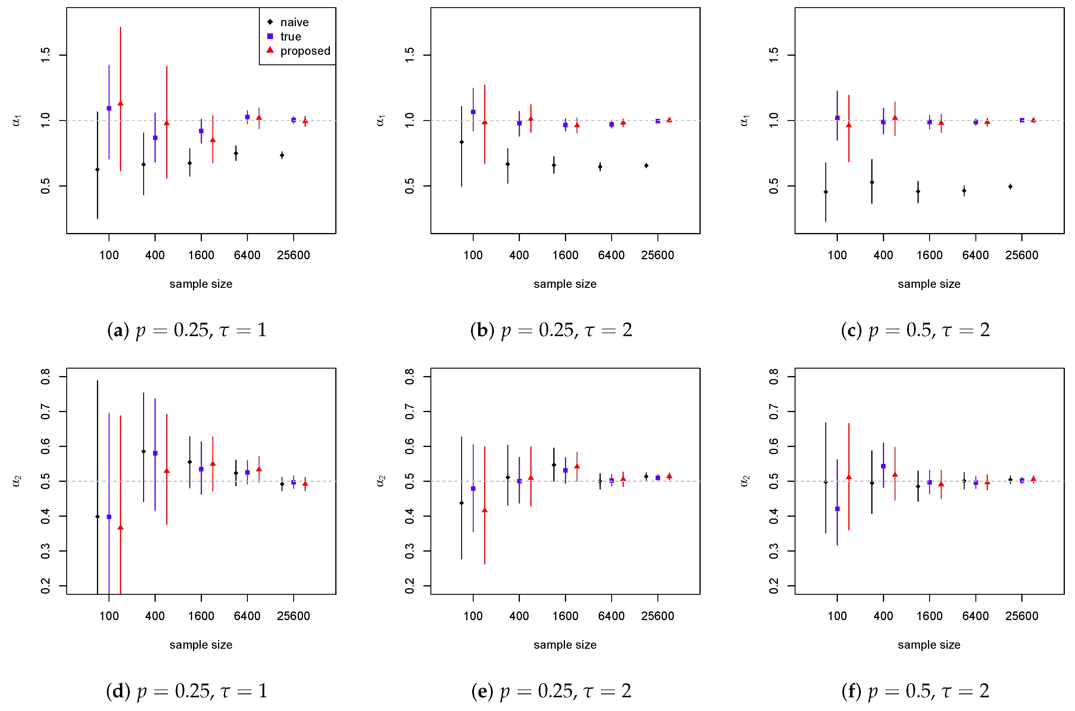
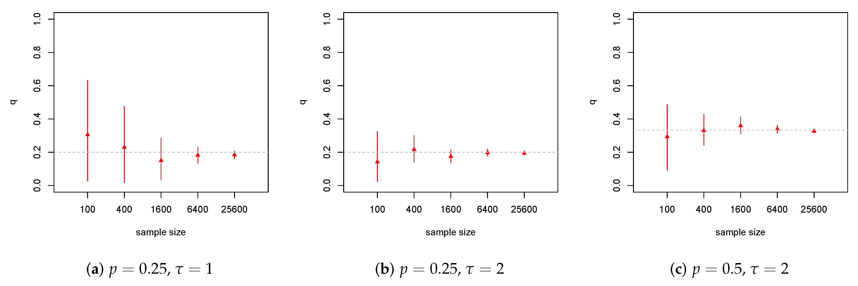
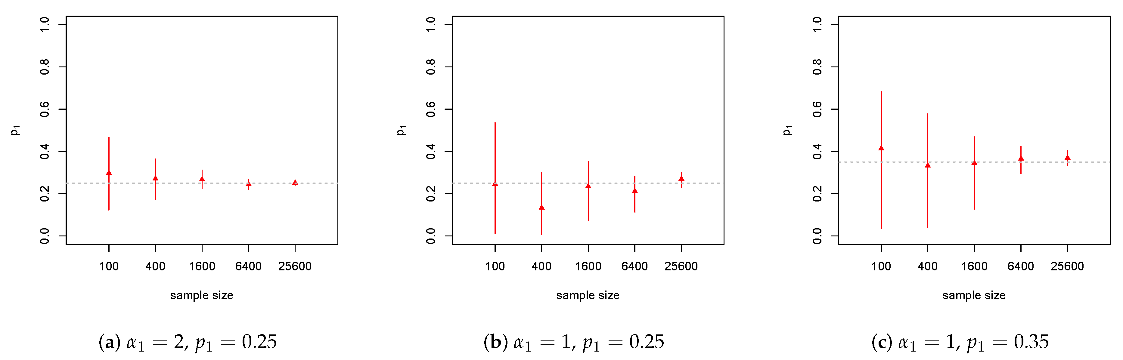
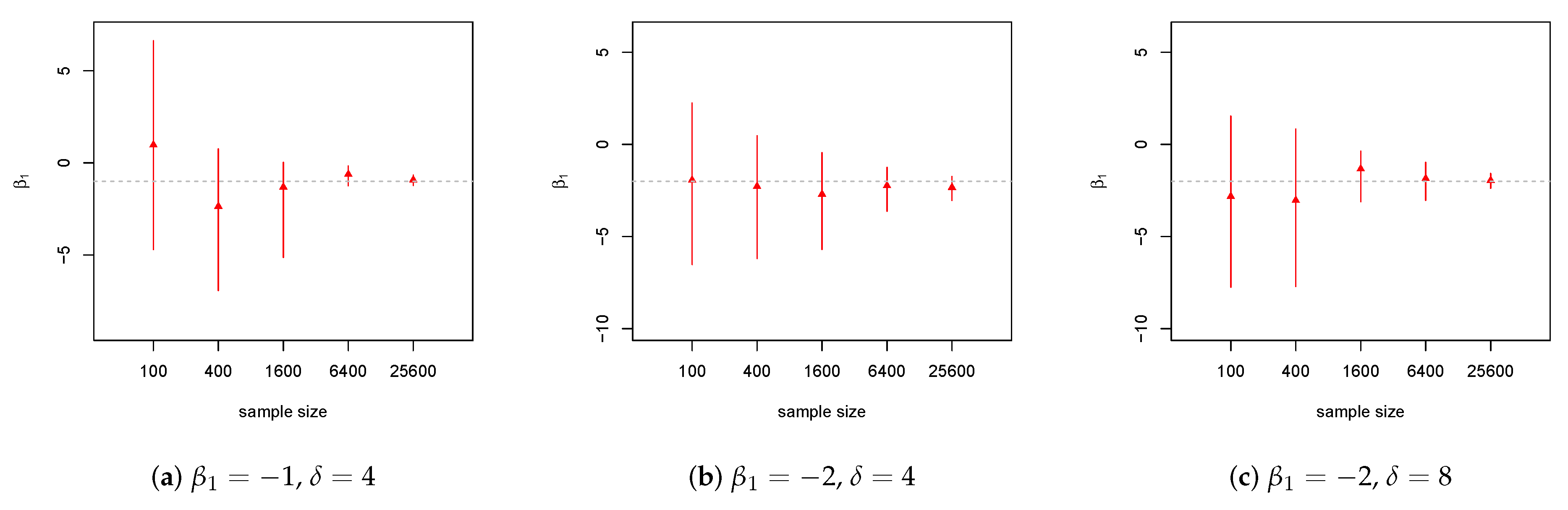
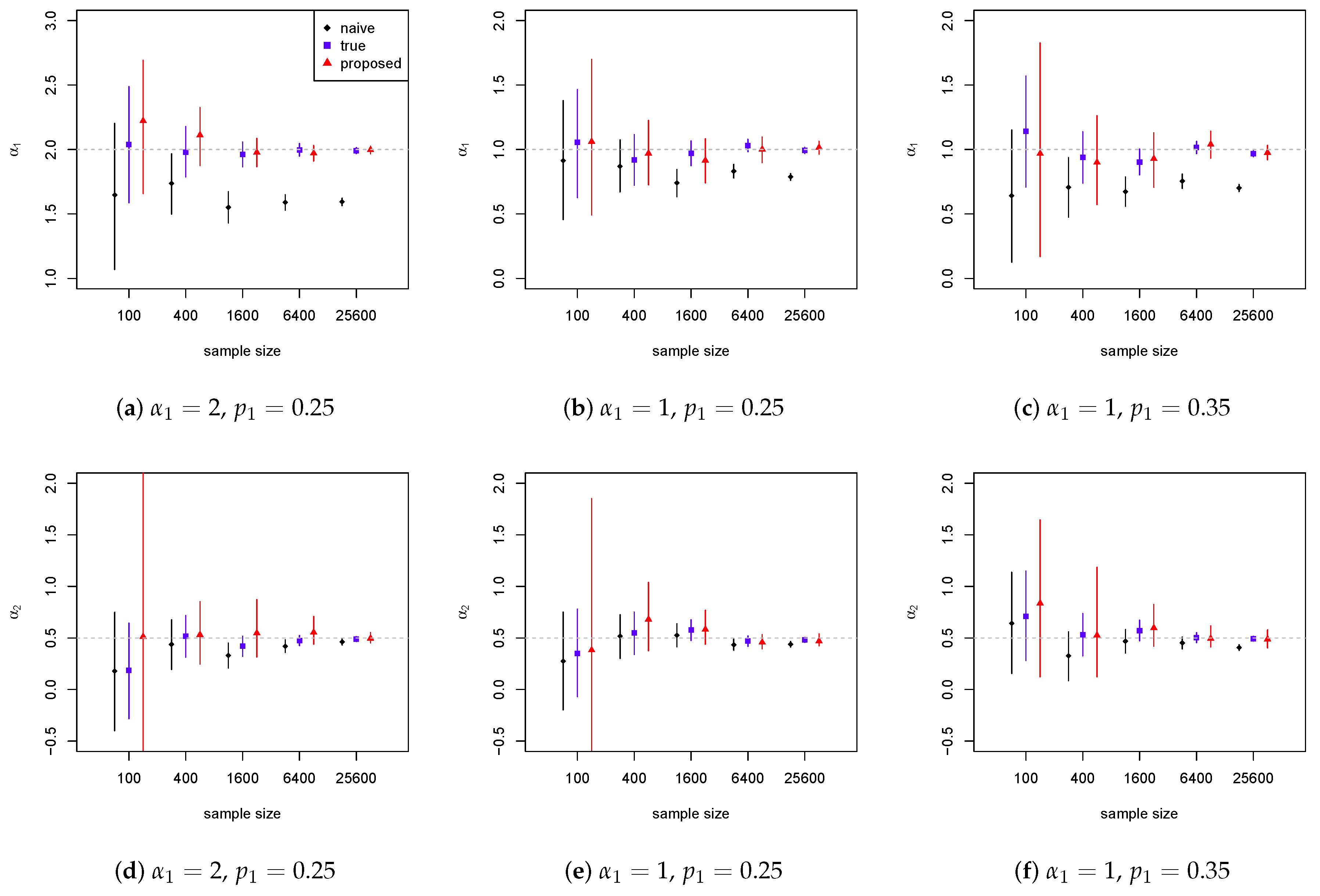
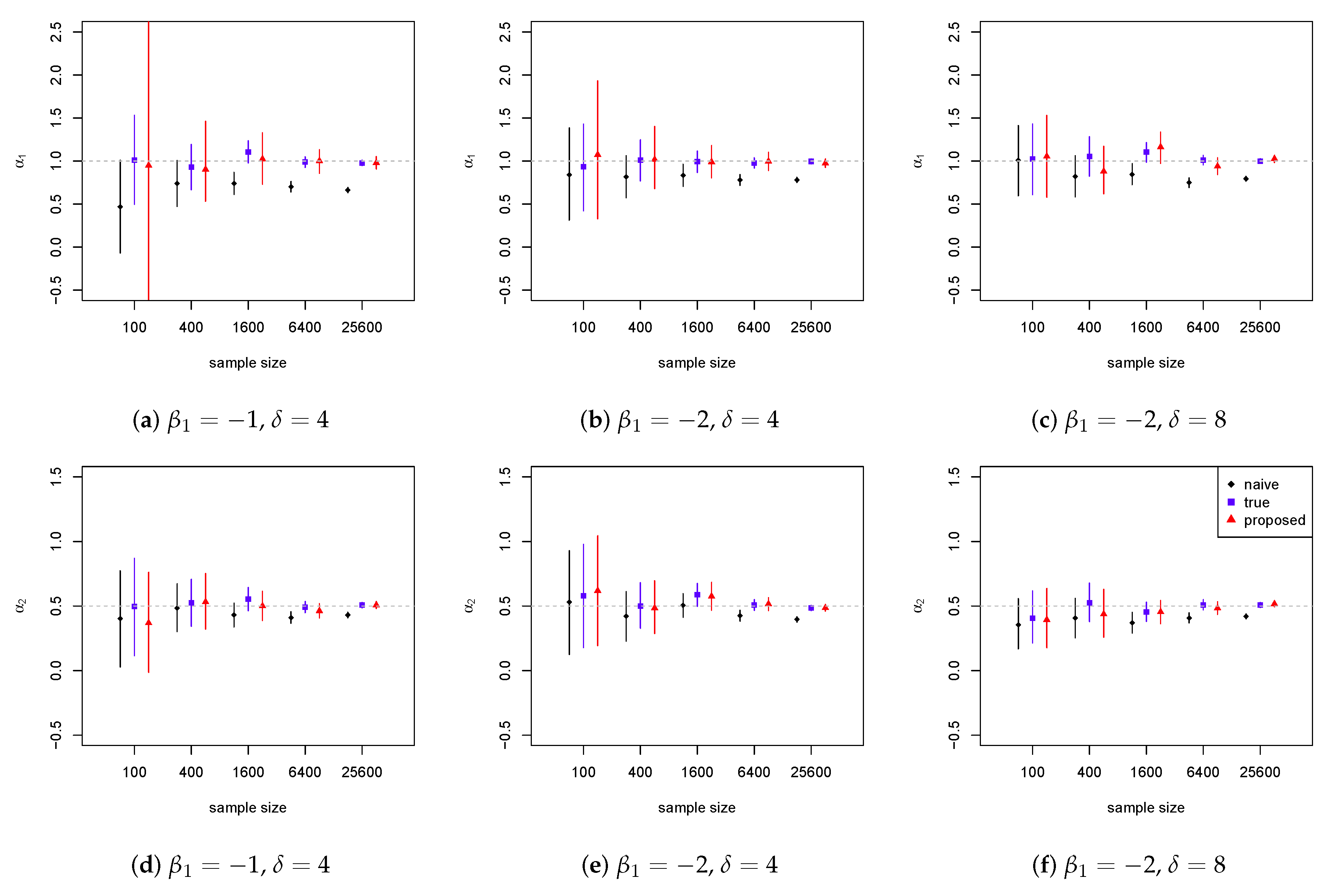
4. Simulation Studies

In order to verify the practical identifiability of the general Weibull, lognormal and two-parameter Pareto models from Section 2, we perform simulation studies to evaluate the learning of the model parameters under finite samples. We fit all the models in WinBUGS called from the R function R2WinBUGS. Details on the BUGS implementation of the heavy-tailed distributions can be found in Scollnik (2001 2002), while those of the misrepresentation model structures are given in Xia et al. (2018).

4.1. Weibull Model

For the Weibull severity model in Example 1, we generate random samples of (V, X, Y) from the true distributional structure and obtain the observed samples of $V^{\ast }$ from those of V using a specific value of p. Based on the conditional distributions of the observed variables, the proposed heavy-tailed model uses the samples of $(Y,V^{\ast },X)$ to estimate the model parameters.

In particular, we generate a single sample of size n for the true risk factor V, using a Bernoulli trial with the probability $\theta =0.5$. Two different values, 0.25 and 0.5, are chosen for the misrepresentation probability p for obtaining the corresponding samples of $V^{\ast }$. The samples of X are generated from a gamma distribution with the shape and scale parameters being (2, 0.5). The corresponding samples of Y are then generated, with the regression coefficients being $({\alpha }_0,{\alpha }_1,{\alpha }_2)=(1.2,1,0.5)$ and the Weibull shape parameter being $\tau =1$ or 2.

We consider the five sample sizes of 100, 400, 1600, 5400 and 25,600. We compare the results from the proposed model in (2) with naive (unadjusted) estimates from Weibull regression using the observed values of $V^{\ast }$ pretending there to be no misrepresentation. We denote the true model as Weibull regression using the “unobserved” values of V generated before obtaining $V^{\ast }$. Independent normal priors with mean zero and variance 10 are used for all the regression coefficients. For the probability parameters p and $\theta$, we use uniform priors on (0, 1). A vague gamma prior with parameters (0.001, 0.001) is specified for $\tau$. We run three chains with randomly-generated initial values and choose a burn-in period of 15,000 and a thinning rate of ×10. Parameter inference is based on 5000 posterior samples that provide an effective sample size over 4500. Figure 1 presents the 95% equal-tailed credible intervals for the regression coefficients ${\alpha }_1$ and ${\alpha }_2$, with the increase of the sample size.

As expected, the naive (unadjusted) estimates are biased downward when compared with those from the true models. That is due to the attenuation effect commonly observed in regression models with mismeasured covariates. For the proposed model, the center of the posterior distribution of ${\alpha }_1$ is very close to that from the true model in most scenarios. The proposed model often gives wider credible intervals, revealing that the existence of the misrepresentation leads to larger uncertainty in the estimation. Since in reality the insurance companies do not observe the true risk status, a large difference in the estimated effects from the naive (unadjusted) model and the proposed model indicates a sustainable underestimation of the risk effect in the unadjusted analysis. This means that the low-risk applicants with a true negative risk status have to overpay their insurance premium for subsiding the underpayment of the applicants who have misrepresented the status.

Figure 2 presents the credible intervals of the prevalence of misrepresentation q from the proposed model. We observe that the credible interval becomes narrower as the sample size increases, with all the intervals covering the true value. When comparing the three panels horizontally, there is larger variability in the estimation for the case with a smaller shape parameter $\tau$ (a) or a larger misclassification probability p (c). Based on the estimate of the prevalence of misrepresentation and the underestimation of the risk effect from the naive (unadjusted) analysis, the insurance companies may be able to estimate the total amount they will be able to recover, by identifying the percentage of applicants who have misrepresented the status.

All in all, the proposed Bayesian model corrects for the attenuation bias from the naive (unadjusted) analysis, while acknowledging the additional variability caused by misrepresentation with wider credible intervals. We observe that the model is able to estimate all the parameters including the true risk effects and the prevalence of misrepresentation, with the width of intervals decreasing at the rate of $\sqrt{1/n}$ in large samples. This confirms the theoretical identifiability we have proven earlier for the models, as well as the classical statistical theories on the speed of convergence for Bayesian estimators.

4.2. Lognormal Model

For the lognormal loss severity model in Example 2, we generate the samples of the true risk statuses $(V_1,V_2)$ with the binomial probabilities being ${\theta }_1=0.5$ and ${\theta }_2=0.4$, respectively. For the misrepresentation probabilities $(p_1,p_2)$, we use two sets of values, $(0.25,0.15)$ and $(0.35,0.25)$. The additional risk factor X is generated from the same distribution as that in the previous subsection. The samples of Y are then generated from the conditional distribution $\left(Y\right|V_1,V_2,X)$, with ${\sigma }^2=1$ and $({\alpha }_0,{\alpha }_1,{\alpha }_2,{\alpha }_3)$$=(-1,1,0.5,1)$ or $(-1,2,0.5,1)$.

The naive (unadjusted) estimates are obtained from lognormal regression using the observed values of $(V_1^{\ast },V_2^{\ast })$, pretending there to be no misrepresentation. We denote the true model as lognormal regression using the corresponding values of $(V_1,V_2)$. The proposed model makes use of the conditional distributions in Equation (5), and treats the true statuses as latent variables. A vague gamma prior is specified for $\tau$ with parameters (0.001, 0.001). Other MCMC details are the same as those for the Weibull model.

Figure 3 presents the 95% equal-tailed credible intervals for the regression coefficients ${\alpha }_1$ and ${\alpha }_2$, with an increasing sample size. For the naive model, we observe a similar attenuation effect in the regression coefficients of $V_1$ and $V_2$, owing to the misrepresentation. The values of the posterior mean of ${\alpha }_1$ and ${\alpha }_2$ from the proposed model are very close to those from the true model in most cases. For the lognormal model, the proposed method gives much wider credible intervals (probably owing to the impact from tail events), when compared with those from a Pareto model with the same structure. Nevertheless, the results for the Pareto model have similar patterns as those in Figure 1 and Figure 2 and, thus, are not presented here. We further observe that the proposed model works better for larger samples, as in the case of large insurance claim data. Since the insurance companies usually do not observe the true risk status, the difference in the estimated effects from the naive (unadjusted) analysis and the proposed model indicates an underestimation of the risk, with the low-risk group being surcharged for subsidizing the misrepresentation group. For the lognormal model, such underestimation occurs in both risk factors subject to misrepresentation.

Figure 4 presents the 95% equal-tailed credible intervals of the misrepresentation probability $p_1$. The results of $p_2$ and the $q_j$’s are similar, and are not presented here. The credible interval becomes narrower as the sample size increases, with all the intervals covering the true value of the probability. In both figures, we observe smaller variability in the estimation for the larger effect case with ${\alpha }_1=2$ and larger variability for the more severe misrepresentation case with $(p_1,p_2)=(0.35,0.25)$. Here, the estimated prevalence of misrepresentation can be used to assess the overall amount the insurance company may be able to recover by identifying the policies with misrepresentation on either of the risk factors.

Similar to the case of the Weibull model, the proposed lognormal model corrects for the attenuation bias from the naive (unadjusted) analysis, confirming the identifiability. The model is able to estimate all the parameters including the true risk effects and misrepresentation probabilities, in the case where there are two risk factors subject to misrepresentation. The width of the interval seems to decrease at the rate of $\sqrt{1/n}$ in large samples, confirming the classical statistical theories on the speed of convergence for Bayesian estimators.

4.3. Pareto Model

For the Pareto model in Example 3, we adopt a different data generation process, as the value of q differs for each observation of X. In particular, we first simulate samples of $V^{\ast }$ from a Bernoulli trial with a probability ${\theta }^{\ast }$ and use them to obtain those of V based on the calculated values of q. The samples of V and X are then used to obtain those for the loss outcome Y.

For the Bernoulli trial, we assume the probability ${\theta }^{\ast }=0.5$ for generating the samples of $V^{\ast }$. The samples of X are generated from the same gamma distribution as that for the Weibull model. For the latent logit model, we assume that the parameters $({\beta }_0,{\beta }_1)$ take two sets of values $(0,-1)$ and $(0,-2)$. For each sample of X, we calculate the prevalence of misrepresentation based on the logit model in Example 3 and obtain the corresponding true samples of V by modifying those of $V^{\ast }$. The corresponding samples of Y are then generated from the conditional distribution $\left(Y\right|V,X)$, assuming $\delta =4$ or 8, the regression coefficients being $({\alpha }_0,{\alpha }_1,{\alpha }_2)$=$(1.2,1,0.5)$. A vague gamma prior with parameters (0.001, 0.001) is specified for $\delta$. Other MCMC details are the same as those adopted for the Weibull and lognormal models.

Figure 5 presents the 95% credible intervals for the regression coefficients ${\alpha }_1$ and ${\alpha }_2$, with the increase of the sample size. For both regression coefficients, we observe that misrepresentation in one risk factor may cause bias in the estimated effects of both the risk factor itself (i.e., the attenuation effect) and the other risk factor. The values of the posterior mean of ${\alpha }_1$ and ${\alpha }_2$ from the proposed model are very close to those from the true model, with slightly longer credible intervals acknowledging the uncertainty due to the existence of misrepresentation. Since the insurance companies do not observe the true risk status, the difference in the estimates from the naive (unadjusted) and adjusted models enables them to assess the bias the misrepresentation has caused in the estimation of the risk effect.

Figure 6 presents the credible intervals of the risk effect ${\beta }_1$ on the prevalence of misrepresentation from the proposed model. The credible interval becomes narrower as the sample size increases, with all the intervals covering the true value. Similar to the findings from Xia et al. (2018), latent models may require a larger sample size to learn the parameters (e.g., ${\beta }_1$) with the same precision, when compared with those from non-latent regression (e.g., ${\alpha }_1$). For heavy-tailed models, the length of the credible intervals may decrease with the sample size in a more erratic manner, due to the impact from tail events. For the latent logit model, the exponential of ${\beta }_1$ quantifies the relative effect on the odds of misrepresentation. When the model includes multiple risk factors, the estimated effects can be used to predict the prevalence of misrepresentation at the policy level, based on various policy characteristics.

Similar to the Weibull and lognormal models, the proposed model corrects for the bias from the naive (unadjusted) analysis that can occur in both risk factors. The model is able to estimate all the parameters including the true risk effects and the risk effect on the prevalence of misrepresentation, in the case where the prevalence of misrepresentation changes with an additional risk factor. The width of the intervals seems to decrease at a rate of $\sqrt{1/n}$ for all the parameters, confirming the classical statistical theories on the speed of convergence for Bayesian estimators.

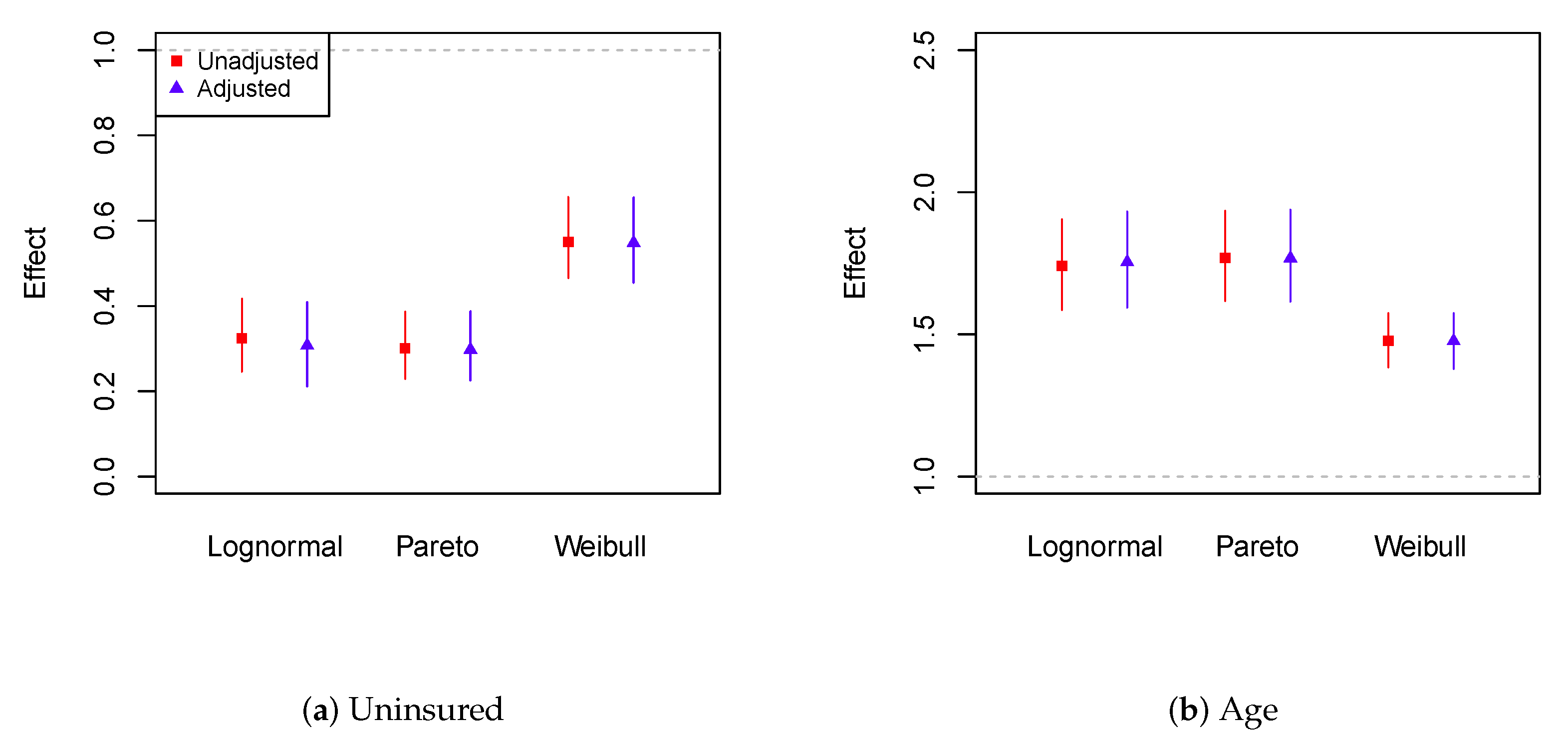
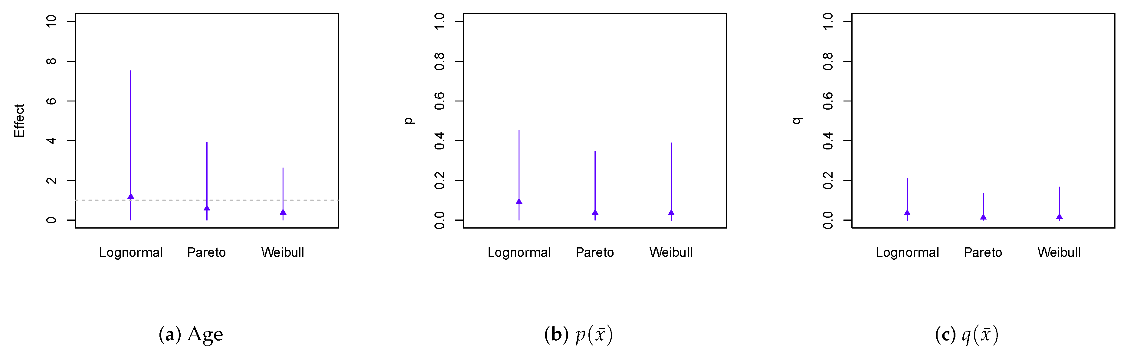
5. Loss Severity Analysis Using Medical Expenditure Data

The Individual Mandate of the Patient Protection and Affordable Care Act (PPACA) implemented a tax penalty for American taxpayers who did not have health insurance, resulting in a motivation to misrepresent the self-reported insurance status. In Sun et al. (2017); Xia and Gustafson (2018), case studies were performed on the potential misrepresentation in the MEPS data concerning the insurance status. The work in Xia and Gustafson (2018) considered the insurance status as the response variable, while Sun et al. (2017) treated the insurance status as the only risk factor in a gamma severity model. Both studies revealed little evidence of the presence of misrepresentation. In the current paper, we use the total medical expenditure variable as our loss severity outcome and include the age and smoking status studied in Xia et al. (2018), which are legitimate rating factors allowed by the PPACA. Most importantly, it will be interesting to perform a model comparison between the gamma model and the heavy-tailed models proposed in this paper.

For the analysis, we include white individuals aged 18–60 who were the reference person in their households. We only include smokers who were more likely to have health expenditures that are heavy-tailed. The sample includes 820 individuals, with 20% identifying themselves as uninsured. We consider the gamma, lognormal, two-parameter Pareto and general Weibull distributions for the medical expenditure variable. We first perform an unadjusted analysis using regular regression based on the four loss distributions. For the adjusted analysis, we adopt the regression structures and misrepresentation setup from Example 3 for each distribution of concern. For the probability $\theta$, we assume a beta prior with both parameters being two (corresponding to a prior mean of 0.5 and the prior standard deviation of 0.224). Other MCMC settings are similar to those in the previous section. For the model comparison,

Table 2. Model selection based on deviance information criterion (DIC) criteria for Bayesian hierarchical models.

DIC	Gamma	Lognormal	Pareto	Weibull
Unadjusted	16,007	15,860	15,865	15,934
Adjusted	16,231	16,357	15,757	16,008

presents the values of the DIC, a goodness of fit criteria similar to AIC and BIC that is appropriate for Bayesian hierarchical models.

Based on the DIC, the Pareto misrepresentation (adjusted) model provides the optimal goodness of fit. For the unadjusted analysis, we observe that the gamma distribution seems to fit the data the worst, consistent with the symmetric densities we obtain on the logarithm of the total expenditures. In addition, the gamma-adjusted model gives extremely large estimates of the misrepresentation probability (over 0.70 with a very narrow credible interval). Due to such contradictory results and the low DIC values associated with the gamma models, we will present only the estimates from the three heavy-tailed models. In Figure 7, we present the 95% equal-tailed credible intervals for the relativity $exp\left({\alpha }_1\right)$ and $exp\left({\alpha }_2\right)$ concerning the effects that the uninsured status and the age have on the average total medical expenditures.

From Figure 7, we observe that the adjusted models give similar estimates of the relative effects, when compared with the unadjusted models. This indicates that the impact from misrepresentation is relatively small. The estimates from the Weibull model seem to differ from those from the other two distributions. For all six models, the uninsured status results in an about 50%–70% decrease in the estimated total medical expenditures. Regarding the age effect, every 12-year increase is expected to result in a 50%–75% increase in the estimated total medical expenditures.

In Figure 8, we present the 95% equal-tailed credible intervals for the relative age effect on the odds of misrepresentation (i.e., $q/(1-q)$), the predicted misrepresentation probability $p\left(\overline{x}\right)$ and the predicted prevalence of misrepresentation $q\left(\overline{x}\right)$ for individuals at the average age of $\overline{x}=42$.

We observe that the age effect is insignificant in predicting the prevalence of misrepresentation q. From the posterior mean of $exp\left({\beta }_1\right)$ from the Pareto model, the odds of misrepresentation decrease by about 50% multiplicatively, when we increase the age by 12 years (one SD). For individuals at the average age, the predicted misrepresentation probability ranges from 3.5%–9.1%, while the predicted prevalence of misrepresentation ranges from 1.3%–3.5% for the three models. Among individuals with an average age who identified themselves as insured, about 1.3%–3.5% of them are estimated to have misrepresented their insurance status. The estimated prevalence is lower than the estimated misrepresentation probability, as the majority of the individuals were insured.

While the impact of misrepresentation and the estimated prevalence of misrepresentation seems to be small, the Pareto misrepresentation model seems to give the best goodness of fit, when compared with the rest of the seven models considered in this section. Due to the small estimates of the prevalence of misrepresentation, the adjustment for misrepresentation seems to result in a very minor impact on the estimated risk effects. This is understandable, as the survey respondents were protected by the Health Insurance Portability and Accountability Act of 1996 and thus had little motivation to misrepresent the insurance status.

6. Conclusions

In the paper, we extend the predictive models of misrepresentation (Xia et al. 2018) to the heavy-tailed regression context. We proved the identifiability of the Weibull, lognormal and Pareto models, confirming that consistent estimation is guaranteed for all the model parameters. Despite the heavy-tailed feature that may cause increased variability in the estimation, the models have anticipated performance under finite samples. With the increase of the sample size, the estimates of all model parameters seemed to converge to their true values, with their standard errors converging to zero. The case study identified the Pareto misrepresentation model as the optimal model in terms of the DIC, revealing the usefulness of modeling the heavy-tailed feature in health expenditure data. From a practical perspective, the proposed models provide important tools for the insurance industry to quantify the impact of misrepresentation, while enabling predictive analytics on the misrepresentation risk at the policy level.

References

1. Ahmad, Khalaf E. 1988. Identifiability of finite mixtures using a new transform. Annals of the Institute of Statistical Mathematics 40: 261–5. [Google Scholar] [CrossRef]
2. Bermúdez, Lluís, and Dimitris Karlis. 2015. A posteriori ratemaking using bivariate Poisson models. Scandinavian Actuarial Journal 2017: 148–58. [Google Scholar]
3. Brockman, M.J., and T.S. Wright. 1992. Statistical motor rating: making effective use of your data. Journal of the Institute of Actuaries 119: 457–543. [Google Scholar] [CrossRef]
4. Chandra, Satish. 1977. On the mixtures of probability distributions. Scandinavian Journal of Statistics 4: 105–12. [Google Scholar]
5. David, Mihaela. 2015. Auto insurance premium calculation using generalized linear models. Procedia Economics and Finance 20: 147–56. [Google Scholar] [CrossRef]
6. Gustafson, Paul. 2014. Bayesian statistical methodology for observational health sciences data. In Statistics in Action: A Canadian Outlook. Edited by Jerald F. Lawless. London: Chapman and Hall/CRC, pp. 163–76. [Google Scholar]
7. Haberman, Steven, and Arthur E. Renshaw. 1996. Generalized linear models and actuarial science. The Statistician 45: 407–36. [Google Scholar] [CrossRef]
8. Hahn, P. Richard, Jared S. Murray, and Ioanna Manolopoulou. 2016. A Bayesian partial identification approach to inferring the prevalence of accounting misconduct. Journal of the American Statistical Association 111: 14–26. [Google Scholar] [CrossRef]
9. Hao, Xuemiao, and Qihe Tang. 2012. Asymptotic ruin probabilities for a bivariate lévy-driven risk model with heavy-tailed claims and risky investments. Journal of Applied Probability 49: 939–53. [Google Scholar] [CrossRef]
10. Hua, Lei. 2015. Tail negative dependence and its applications for aggregate loss modeling. Insurance: Mathematics and Economics 61: 135–45. [Google Scholar] [CrossRef]
11. Jiang, Wenxin, and Martin A. Tanner. 1999. On the identifiability of mixtures-of-experts. Neural Networks 12: 1253–8. [Google Scholar] [CrossRef]
12. Klein, Nadja, Michel Denuit, Stefan Lang, and Thomas Kneib. 2014. Nonlife ratemaking and risk management with bayesian generalized additive models for location, scale, and shape. Insurance: Mathematics and Economics 55: 225–49. [Google Scholar] [CrossRef]
13. Peng, Liang, and Yongcheng Qi. 2017. Inference for Heavy-Tailed Data: Applications in Insurance and Finance. Cambridge: Academic Press. [Google Scholar]
14. Qi, Yongcheng. 2010. On the tail index of a heavy tailed distribution. Annals of the Institute of Statistical Mathematics 62: 277–98. [Google Scholar] [CrossRef]
15. Scollnik, David P.M. 2001. Actuarial modeling with MCMC and BUGS. North American Actuarial Journal 5: 96–124. [Google Scholar] [CrossRef]
16. Scollnik, David P.M. 2002. Modeling size-of-loss distributions for exact data in WinBUGS. Journal of Actuarial Practice 10: 202–27. [Google Scholar]
17. Scollnik, David P.M. 2015. A Pareto scale-inflated outlier model and its Bayesian analysis. Scandinavian Actuarial Journal 2015: 201–20. [Google Scholar] [CrossRef]
18. Sun, Liangrui, Michelle Xia, Yuanyuan Tang, and Philip G. Jones. 2017. Bayesian adjustment for unidirectional misclassification in ordinal covariates. Journal of Statistical Computation and Simulation 87: 3440–68. [Google Scholar] [CrossRef]
19. Xia, Michelle, and Paul Gustafson. 2016. Bayesian regression models adjusting for unidirectional covariate misclassification. The Canadian Journal of Statistics 44: 198–218. [Google Scholar] [CrossRef]
20. Xia, Michelle, and Paul Gustafson. 2018. Bayesian inference for unidirectional misclassification of a binary response trait. Statistics in Medicine 37: 933–47. [Google Scholar] [CrossRef] [PubMed]
21. Xia, Michelle, Lei Hua, and Gary Vadnais. 2018. Embedded predictive analysis of misrepresentation risk in GLM ratemaking models. Variance: Advancing the Science of Risk. in press. [Google Scholar]
22. Yang, Yang, Kaiyong Wang, Jiajun Liu, and Zhimin Zhang. 2018. Asymptotics for a bidimensional risk model with two geometric lévy price processes. Journal of Industrial & Management Optimization, 765–72. [Google Scholar] [CrossRef]
Figure 1. Credible intervals for the risk effects of V (top) and X (bottom) for theWeibull loss severity model. The dashed line marks the true value.
Risks 06 00083 g001
Figure 2. Credible intervals for the prevalence of misrepresentation q for the Weibull loss severity model.
Risks 06 00083 g002
Figure 3. Credible intervals for the risk effects of V1 (top) and V2 (bottom) for the lognormal loss severity model. The dashed line marks the true value.
Risks 06 00083 g003
Figure 4. Credible intervals for the misrepresentation probability p1 for the lognormal loss severity model.
Risks 06 00083 g004
Figure 5. Credible intervals for the risk effects of V (top) and X (bottom) for the Pareto loss severity model. The dashed line marks the true value.
Risks 06 00083 g005
Figure 6. Credible intervals for the risk effect β1 on the prevalence of misrepresentation for the Pareto loss severity model.
Risks 06 00083 g006
Figure 7. Credible intervals for the relativity of uninsured status and age, exp(α1) and exp(α2), for the heavy-tailed models on the total medical expenditures. The age effect corresponds to the increase of age by one standard deviation (i.e., SD = 12 years).
Risks 06 00083 g007
Figure 8. Credible intervals for the age effect exp(β1) on the odds of misrepresentation, the predicted misrepresentation probability p ( x ¯ ) and the prevalence of misrepresentation q ( x ¯ ) for individuals at the average age of 42.
Risks 06 00083 g008