Abstract
We present a stochastic simulation forecasting model for stress testing that is aimed at assessing banks’ capital adequacy, financial fragility, and probability of default. The paper provides a theoretical presentation of the methodology and the essential features of the forecasting model on which it is based. Also, for illustrative purposes and to show in practical terms how to apply the methodology and the types of outcomes and analysis that can be obtained, we report the results of an empirical application of the methodology proposed to the Global Systemically Important Banks (G-SIB) banks. The results of the stress test exercise are compared with the results of the supervisory stress tests performed in 2014 by the Federal Reserve and EBA/ECB.
Keywords:
capital adequacy; economic capital; financial fragility; liquidity risk; Monte Carlo simulation; probability of default; Solvency risk; SREP; stochastic simulation; stress testing JEL Classification:
C15; C63; G21; G28; G32
1. Introduction
The aim of this paper is to propose a new approach to banks stress testing and assessment of a bank’s financial fragility that overcomes some of the limitations of current methodologies. In consideration of the surging relevance that stress tests are assuming in determining the banks capital endowment, it is extremely important that this kind of exercises will be performed through a methodological approach that is capable of effectively catching the overall degree of a bank’s financial fragility.
We reject the idea that it is possible to adequately measure banks’ financial fragility degree by looking at one adverse scenario (or a very limited number of them), being solely driven by macroeconomic assumptions, and by assessing capital impact through a building block approach made up of a set of different silos based single risk models (i.e., simply aggregating risk measures obtained from distinct models run separately). Current stress testing methodologies are designed to indicate the potential capital impact of one specific predetermined scenario, but they fail in adequately measuring banks’ degree of forward looking financial fragility, providing poor indications in this regard, especially when the cost in terms of time and effort required is considered1.
We present a stochastic model to develop multi-period forecasting scenarios in order to stress test banks’ capital adequacy with respect to all of the relevant risk factors that may affect capital, liquidity, and regulatory requirements. All of the simulation impacts are simultaneously determined within a single model, overcoming dependence on a single macroeconomic scenario and providing coherent results on the key indicators in all periods and in a very large number of different possible scenarios, being characterized by different level of severity and covering extreme tail events as well. We show how the proposed approach enables a new kind of solution to assess banks’ financial fragility, given by the estimated forward-looking probability of breach of regulatory capital ratios, probability of default and probability of funding shortfall.
The stochastic simulation approach that is proposed in this paper is based on our previous research, initially developed to assess corporate probability of default2 and then extended to the particular case of financial institutions.3 In the present work, we have further developed and tested the modeling within a broader banking stress testing framework.
We begin in Section 2 with a brief overview of the main limitations and shortcomings of current stress testing methodologies; then, in Section 3, we describe the new methodology, the key modeling relations necessary to implement the approach and the stochastic simulation outputs. Afterwards, in Section 4 and Section 5, we present an empirical application of the stress testing methodology proposed for G-SIB banks; the exercise is essentially intended to show how the method can be practically applied, although in a very simplified way, and does not represent to any extent a valuation on the capital adequacy of the banks considered; rather, it is to be considered solely as an example for illustrative purposes, and the specific assumptions adopted must be considered as only one possible sensible set of assumptions, and not as the only or best implementation paradigm. In this section, we also compare the results of our stress test with those from the supervisory stress test performed on United Stated (US) banks by the Federal Reserve (published in March 2014) and those from the EBA/ECB stress test on European Union (EU) banks (published in October 2014). Furthermore, we also provide some preliminary back-testing evidence on the reliability of new proposed approach, by applying it to a few famous banks default cases and by comparing the results obtained with market dynamics. Section 6 ends the paper with some conclusive considerations and remarks. Appendix A and Appendix B contains all of the assumptions related to the empirical exercise performed, while further results and outputs of the exercise are reported in Appendix C.
2. The Limitations of Current Stress Testing Methodologies: Moving towards a New Approach
Before beginning to discuss stress testing, it is worth clarifying what we mean by bank stress testing, and what purposes in our opinion this kind of exercise should serve. In this work, we focus solely on bank-wide stress testing aimed at assessing the overall capital adequacy of a bank, and in this regard, we define stress testing as an analytical technique designed to assess a bank’s capital and liquidity degree of fragility against “all” potential future adverse scenarios, with the aim of supporting supervisory authorities and/or management to evaluate the bank’s forward looking capital adequacy in relation to a preset level of risk.
Current bank capital adequacy stress testing methodologies are essentially characterized by the following key features:4
- The consideration of only one deterministic adverse scenario (or at best a very limited number, 2, 3, … scenarios), limiting the exercise’s results to one specific set of stressed assumptions.
- The use of macroeconomic variables as stress drivers (GDP, interest rate, exchange rate, inflation rate, unemployment, etc.), which must then be converted into bank-specific micro risk factor impacts (typically credit risk and market risk impairments, net interest income, regulatory requirement) by recurring to satellite models (generally based on econometric modeling).
- The total stress test capital impact is determined by adding up through a building block framework the impacts of the different risk factors, each of which is estimated through specific and independent silo-based satellite models.
- The satellite models are often applied with a bottom-up approach (especially for credit and market risk), i.e., using a highly granular data level (single client, single exposure, single asset, etc.) to estimate the stress impacts and then adding up all of the individual impacts.
- In supervisory stress tests, the exercise is performed by the banks and not directly by supervisors, the latter setting the rules and assumptions and limiting their role in checking oversight and challenging how banks apply the exercise rules.
This kind of stress testing approach presents the following shortcomings:
- The exclusive focus of the stress testing exercise on one single or very few worst-case scenarios is probably the main limit of the current approach and precludes its use to adequately assess banks’ financial fragility in broader terms; the best that can be achieved is to verify whether a bank can absorb losses related to that specific set of assumptions and level of stress severity. But, a bank can be hit by a potentially infinite number of different combinations of adverse dynamics in all of the main micro and macro variables that affect its capital. Moreover, a specific worst-case scenario can be extremely adverse for some banks particularly exposed to those risk factors stressed in the scenario, but not for other banks that are less exposed to those factors, but this does not mean that the former banks are, in general, more fragile than the latter; the reverse may be true in other worst-case scenarios. This leads to the thorny issue of how to establish the adverse scenario. What should the relevant adverse set of assumptions be? Which variables should be stressed, and what severity of stress should be applied? This issue is particularly relevant for supervisory authorities when they need to run systemic stress testing exercises, with the risk of setting a scenario the may be either too mild or excessively adverse. Since we do not know what will happen in the future, why should we check for just one single combination of adverse impacts? The “right worst-case scenario” simply does not exist, the ex-ante quest to identify the financial system’s “black swan event” can be a difficult and ultimately useless undertaking. In fact, since banks are institutions in a speculative position by their very nature and structure,5 there are many potential shocks that may severely hit them in different ways. In this sense, the black swan is not that rare, so to focus on only one scenario is too simplistic and intrinsically biased.
- Another critical issue that is related to the “one scenario at a time” approach is that it does not provide the probability of the considered stress impact’s occurrence, lacking the most relevant and appropriate measure for assessing the bank’s capital adequacy and default risk: Current stress test scenarios do not provide any information about the assigned probabilities; this strongly reduces the practical use and interpretation of the stress test results. Why are probabilities so important? Imagine that some stress scenarios are put into the valuation model. It is impossible to act on the result without probabilities: in current practice, such probabilities may never be formally declared. This leaves stress testing in a statistical purgatory. We have some loss numbers, but who is to say whether we should be concerned about them?6 In order to make a proper and effective use of stress test results, we need an output that is expressed in terms of probability of infringing the preset capital adequacy threshold.
- The general assumption that the main threat to banking system stability is typically due to exogenous shock stemming from the real economy can be misleading. In fact, historical evidence and academic debate make this assumption quite controversial.7 Most of the recent financial crises (including the latest) were not preceded (and therefore not caused) by a relevant macroeconomic downturn; generally, quite the opposite was true, i.e., endogenous financial instability caused a downturn in the real economy.8 Hence, the practice of using macroeconomic drivers for stress testing can be misleading because of the relevant bias in the cause-effect linkage, but on closer examination, it also turns out to be an unnecessary additional step with regard to the test’s purpose. In fact, since the stress test ultimately aims to assess the capital impact of adverse scenarios, it would be much better to directly focus on the bank-specific micro variables that affect its capital (revenues, credit losses, non-interest expenses, regulatory requirements, etc.). Working directly on these variables would eliminate the risk of potential bias in the macro-micro translation step. The presumed robustness of the model and the safety net of having an underlying macroeconomic scenario within the stress test fall short, while considering that: (a) we do not know which specific adverse macroeconomic scenario may occur in the future; (b) we have no certainty about how a specific GDP drop (whatever the cause) affects net income; (c) we do not know/cannot consider all other potential and relevant impacts that may affect net income beyond those that are considered in the macroeconomic scenario. Therefore, it is better to avoid expending time and effort in setting a specific macroeconomic scenario from which all impacts should arise, and to instead try to directly assess the extreme potential values of the bank-specific micro variables. Within a single-adverse-scenario approach, the macro scenario definition has the scope of ensuring comparability in the application of the exercise to different banks and to facilitate the stress test storytelling rationale for supervisor communication purposes.9 However, within the multiple scenarios approach that is proposed, which no longer needs to exist, there are other ways to ensure comparability in the stress test. Of course, the recourse to macroeconomic assumptions can also be considered in the stochastic simulation approach proposed, but as we have explained, it can also be avoided; in the illustrative exercise presented below, we avoided modeling stochastic variables in terms of underlying macro assumptions, to show how we can dispense with the false myth of the need for a macro scenario as the unavoidable starting point of the stress test exercise.
- Recourse to a silo-based modeling framework to assess the risk factor capital impacts with aggregation through a building block approach does not ensure a proper handling of risk integration10 and is unfit to adequately manage the non-linearity, path dependence, feedback and cross-correlation phenomena that strongly affects capital in “tail” extreme events. This kind of relationships assumes a growing relevance with the extension of the stress test time horizon and severity. Therefore, a necessary step to properly capture the effects of these phenomena in a multi-period stress test is to abandon the silo-based approach and to adopt an enterprise risk management (ERM) model, which, within a comprehensive unitary model, allows for us to manage the interactions among the fundamental variables, integrating all risk factors and their impacts in terms of P&L-liquidity-capital-requirements11.
- The bottom-up approach to stress test calculations generally entails the use of satellite econometric models in order to translate macroeconomic adverse scenarios into granular risk parameters, and internal analytical risk models to calculate impairments and regulatory requirements. The highly granular data level employed and the consequent use of the linked modeling systems makes stress testing exercises extremely laborious and time-consuming. The high operational cost that is associated with this kind of exercise contributes to limiting analysis to one or few deterministic scenarios. In addition, the high level of fragmentation of input data and the long calculation chain increases the risk of operational errors and makes the link between adverse assumptions and final results less clear. The bottom-up approach is well suited for current-point-in-time analysis characterized by a short-term forward-looking risk analysis (e.g., one year for credit risk); the extension of the bottom-up approach into forecasting analysis necessarily requires a static balance sheet assumption, otherwise the cumbersome modeling systems would lack the necessary data inputs. But, the longer the forecasting time horizon considered (2, 3, 4, … years), the less sense that it makes to adopt a static balance sheet assumption, compromising the meaningfulness of the entire stress test analysis. The bottom-up approach loses its strength when these shortcomings are considered, generating a false sense of accuracy with considerable unnecessary costs.
- In consideration of the use of macroeconomic adverse scenario assumptions and the bottom-up approach that is outlined above, supervisors are forced to rely on banks’ internal models to perform stress tests. Under these circumstances, the validity of the exercise depends greatly on how the stress test assumptions are implemented by the banks in their models, and on the level of adjustments and derogations they applied (often in an implied way). Clearly, this practice leaves open the risk of moral hazard in stress test development and conduct, and it also affects the comparability of the results, since the application of the same set of assumptions with different models does not ensure a coherent stress test exercise across all of the banks involved.12 Supervisory stress testing should be performed directly by the competent authority. In order to do so, they should adopt an approach that does not force them to depend on banks for calculations.13
The stress testing approach proposed in this paper aims to overcome the limits of current methodologies and practices highlighted above.
3. Analytical Framework
3.1. Stochastic Simulation Approach Overview
In a nutshell, the proposed approach is based on a stochastic simulation process (generated using the Monte Carlo method), applied to an enterprise-based forecasting model, which generates thousands of different multi-period random scenarios, in each of which coherent projections of the bank’s income statement, balance sheet and regulatory capital are determined. The random forecast scenarios are generated by modeling all of the main value and risk drivers (loans, deposits, interest rates, trading income and losses, net commissions, operating costs, impairments and provisions, default rate, risk weights, etc.) as stochastic variables. The simulation results consist of distribution functions of all the output variables of interest: capital ratios, shareholders equity, CET1 (Common Equity Tier 1), net income and losses, cumulative losses related to a specific risk factor (credit, market, ...), etc. This allows for us to obtain estimates of the probability of occurrence of relevant events, such as breach of capital ratios, default probability, CET1 ratio below a preset threshold, liquidity indicators above or below preset thresholds, etc.
The framework is based on the following features:
- Multi-period stochastic forecasting model: a forecasting model to develop multiple scenario projections for income statement, balance sheet and regulatory capital ratios, capable of managing all of the relevant bank’s value and risk drivers in order to consistently ensure:
- a dividend/capital retention policy that reflects regulatory capital constraints and stress test aims;
- the balancing of total assets and total liabilities in a multi-period context, so that the financial surplus/deficit generated in each period is always properly matched to a corresponding (liquidity/debt) balance sheet item; and,
- the setting of rules and constraints to ensure a good level of intrinsic consistency and correctly manage potential conditions of non-linearity. The most important requirement of a stochastic model lies in preventing the generation of inconsistent scenarios. In traditional deterministic forecasting models, consistency of results can be controlled by observing the entire simulation development and set of output. However, in stochastic simulation, which is characterized by the automatic generation of a very large number of random scenarios, this kind of consistency check cannot be performed, and we must necessarily prevent inconsistencies ex-ante within the model itself, rather than correcting them ex-post. In practical terms, this entails introducing into the model rules, mechanisms and constraints that ensure consistency, even in stressed scenarios.14
- Forecasting variables expressed in probabilistic terms: the variables that represent the main risk factors for capital adequacy are modeled as stochastic variables and defined through specific probability distribution functions in order to establish their future potential values, while interdependence relations among them (correlations) are also set. The severity of the stress test can be scaled by properly setting the distribution functions of stochastic variables.
- Monte Carlo simulation: this technique allows us to solve the stochastic forecast model in the simplest and most flexible way. The stochastic model can be constructed using a copula-based or other similar approaches, with which it is possible to express the joint distribution of random variables as a function of the marginal distributions.15 Analytical solutions—assuming that it is possible to find them—would be too complicated and strictly bound to the functional relation of the model and of the probability distribution functions adopted, so that any changes in the model and/or probability distribution would require a new analytical solution. The flexibility provided by the Monte Carlo simulation, however, allows for us to very easily modify stress severity and the stochastic variable probability functions.
- Top-down comprehensive view: the simulation process set-up utilizes a high level of data aggregation, in order to simplify calculation and guarantee an immediate view of the causal relations between input assumptions and results. The model setting adheres to an accounting-based structure, aimed at simulating the evolution of the bank’s financial statement items (income statement and balance sheet) and regulatory figures and related constraints (regulatory capital, RWA–Risk Weighted Assets, and minimum requirements). An accounting-based model has the advantage of providing an immediately-intelligible comprehensive overview of the bank that facilitates the standardization of the analysis and the comparison of the results.16
- Risk integration: the impact of all the risk factors is determined simultaneously, consistently with the evolution of all of the economics within a single simulation framework.
In the next section, we will describe in formal terms the guidelines to follow in developing the forecasting model and the risk factor modeling in the stress test. The empirical exercise that is presented in the following section will clarify how to practically handle these issues.
3.2. The Forecasting Model
Here, we formally present the essential characteristics of a multi-period forecasting model that is suited to determine the consistent dynamics of a bank’s capital and liquidity excess/shortfall. This requires prior definition of the basic economic relations that rule the capital projections and the balancing of the bank’s financial position over a multi-period time horizon. We develop a reduced-form model that is aimed at straightforwardly presenting the rationale according to which these key features must be modeled.
The Equity Book Value represents the key figure for determining a bank’s solvency and in each period, it is a function of its value in the previous period, Net Income/losses and dividend payout. We consider Net Income to be conditioned by some elements of uncertainty, the dynamics of which can be described through a series of stochastic processes with discrete parameters, of which we assume that the information necessary to define them is known. In the following Section 3.3, we provide a brief description of the stochastic variables considered in the model. Of course, the Net Income dynamic will also affect, through the Equity Book Value, liabilities, and assets in the bank’s balance sheet; here below, we provide a description of the main accounting relationships that rule the forecasting model. We consider that a bank’s abridged balance sheet can be described by the following identity:
The equity book value represents the amount of equity and reserve available to the bank to cover its capital needs. Therefore, in order to model the evolution of equity book value we must first determine the bank’s regulatory capital needs, and in this regard, we must consider both capital requirements (i.e., all regulatory risk factors: credit risk, market risk, operational risk, and any other additional risk requirements) and all of those regulatory adjustments that must be applied to equity book value in order to determine regulatory capital in terms of common equity tier 1, or common equity tier 1 adjustments (i.e., intangible assets, IRB shortfall of credit risk adjustments to expected losses), regulatory filters, deductions, etc.).
We can define the target level of common equity tier 1 capital (CET1) as a function of regulatory requirements and the target capital ratio through the following formula:
where represents the risk weight factor and is the common equity tier 1 ratio target, the latter depending on the minimum regulatory constraint (the minimum capital threshold that by law the bank must hold), plus a capital buffer set according to market/shareholders/management risk appetite.
Now, we can determine the equity book value that the bank must hold in order to reach the regulatory capital ratio target set in Equation (2) as:
Equation (3) sets a capital constraint expressed in terms of equity book value necessary to achieve the target capital ratio; as we shall see later on, this constraint determines the bank’s dividend/capital retention policy.
In each forecasting period, the model has to ensure a financial balance, which means a matching between cash inflow and outflow. We assume for the sake of simplicity that the asset structure is exogenously determined in the model, and thus that financial liabilities change accordingly in order to balance as plug-in variables.17 Assuming that there are no capital transactions (equity issues or buy-backs), the bank’s funding needs—additional funds needed (AFN)—represents the financial surplus/deficit generated by the bank in each period and is determined by the following expression:
A positive value represents the new additional funding necessary in order to finance all assets at the end of the period, while a negative value represents the financial surplus that is generated in the period. The forward-looking cash inflow and outflow balance constraint can be defined as:
Equation (5) expresses a purely financial equilibrium constraint, which is capable of providing a perfect match between total assets and total liabilities.18
The basic relations necessary to develop balance sheet projections within the constraints set in (3) and (5) can be expressed in a reduced form as:
Equation (6) represents the bank’s excess capital, or the equity exceeding target capital needs and thus available for paying dividends to shareholders. The bank has a capital shortfall in relation to its target capital ratio whenever Equation (3) is not satisfied, or:
The outlined capital retention modeling allows for us to project consistent forecasting financial statements in a multi-period context; this is a necessary condition for unbiased long term stress test analysis, especially within a stochastic simulation framework. In fact, consider that, while for short-term analysis, the simple assumption of setting a zero-dividend distribution can be considered as reasonable and unbiased, in a multi-period analysis we cannot assume that the bank will never pay any dividend during the positive years if there is available excess capital; and, of course, any distribution reduces the capital available afterward to face adverse scenarios. An incorrect modeling of dividend policy rules may bias the results; for example, assuming within a stochastic simulation a fixed payout not linked to net income and capital requirements may generate inconsistent scenarios, in which the bank pays dividends under conditions that would not allow for any distribution.
3.3. Stochastic Variables and Risk Factors Modeling
Not all of the simulation’s input variables need to be explicitly modeled as stochastic variables; some variables can also be functionally determined within of the forecasting model, by being linked to the value of other variables (for example, in terms of relationship to or percentage of a stochastic variable), or expressed in terms of functions of a few key figures or simulation outputs.19
Generally speaking, the stochastically-modeled variables will be those with the greatest impact on the results and those of which the future value is most uncertain. For the purposes of the most common types of analysis, stochastic variables will certainly include those that characterize the typical risks of a bank and be considered within prudential regulation (credit risk on loans, market and counterparty risk on securities held in trading and banking book, operational risk).
The enterprise-based approach adopted allows for us to manage the effects of the overall business dynamics of the bank, including those impacts not considered as Pillar I risk factors, and depending on variables, such as swing in interest rates and spreads, volume change in deposits and loans, swing in net commissions, operating costs, and non-recurring costs. The dynamics of all these Pillar II risk factors are managed and simulated jointly with the traditional Pillar I risk factors (market and credit) and other additional risk factors (e.g., reputational risk,20 strategic risk, compliance risk, etc.).
Table 1 shows the main risk factors of a bank (both Pillar I and II), highlighting the corresponding variables that impact income statement, balance sheet, and RWA. For each variable, the variables that best sum up their representation and modeling are highlighted, and alongside them, possible modeling breakdown and/or evolution. For example, the dynamics of credit risk impacts on loans can be viewed at the aggregate (total portfolio) level, acting on a single stochastic variable representing total credit adjustments, or can be managed by one variable for each sufficiently-large portfolio characterized by specific risk, based on the segmentation most suited to the situation under analysis; for example, the portfolio can be breakdown by type of: client (retail, corporate, SME, etc.); product (mortgages, short-term uses, consumer, leasing, etc.); geographic area; subsidiaries; and, etc. The modeling of loan-loss provisions and regulatory requirements can be handled in a highly simplified way—for example, using an accounting-based loss approach (i.e., loss rate, charge-off and recovery) and a simple risk weight—or a more sophisticated one—for example, through an expected loss approach as a function of three components: PD, LGD, and EAD; for further explanations, see Appendix A.

Table 1.
Stress test framework: risk factor modeling.
The probability distribution function must be defined for each stochastic variable in each simulation forecast period—in essence, a path of evolution of the range of possible values the variable can take on over time must be defined.
By assigning appropriate ranges of variability to the distribution function, we can calibrate the severity of the stress test according to the aims of our analysis. Developing several simulations that are characterized by increasingly levels of severity can provide a more complete picture of a bank’s capital adequacy, as it helps us to better understand the effects in the tail of the simulation and to verify how conditions of non-linearity impact the bank’s degree of financial fragility.
A highly effective and rapid way to further concentrate the generation of random scenarios within a pre-set interval of stress is to limit the distribution functions of stochastic variables to an appropriate range of values. In fact, the technique of truncation function allows for us to restrict the domain of probability distributions to within the limits of values comprised between a specific pair of percentiles. We can thus develop simulations that are characterized by a greater number of scenarios generated in the distribution tails, and therefore with more robust results under conditions of stress.
Once the distribution functions of the stochastic variables have been defined, we must then specify the correlation coefficients between variables (cross correlation) and over time (autocorrelation). In order to set these assumptions, we can turn to historical estimates of relationships of variables over time, and to direct forecasts based on available information and on the possible types of relationships that can be foreseen in stressed conditions. However, it is important to remember that correlation is a scalar measure of the dependency between two variables, and thus cannot tell us everything about their dependence structure.21 Therefore, it is preferable that the most relevant and strongest relationships of interdependence be directly expressed—to the highest degree possible—within the forecast model, through the definition of appropriate functional relationships among variables. This in itself reduces the need to define relationships of dependency between variables by means of correlation coefficients, or at least change the terms of the problem.
For a few concrete examples of how the necessary parameters can be set to define the distribution functions of various stochastic variables and the correlation matrix, see Appendix A.
3.4. Results of Stochastic Simulations
The possibility of representing results in the form of a probability distribution notably augments the quantity and quality of information that is available for analysis, allowing for us to develop new solutions to specific problems that could not be obtained with traditional deterministic models. For example, we can obtain an ex-ante estimate of the probability that a given event, such as the triggering of a relevant capital ratio threshold, or a default, will occur. In stress testing for capital adequacy purposes, the distribution functions of all capital ratios and regulatory capital figures will be of particular importance. Here below we provide a brief description of some solutions that could be particularly relevant with regard to stress testing for capital and liquidity adequacy purposes.
3.4.1. Probability of Regulatory Capital Ratio Breach
On the basis of the capital ratio probability distribution simulated, we can determine the estimated probability of triggering a preset threshold (probability of breach), such as the minimum regulatory requirement or the target capital ratio. The multi-period context allows for us to estimate cumulated probabilities according to the relevant time period (one year, two years, …. n years), thus the CET1 ratio probability of breach in each period can be defined as:
where is the preset threshold.
Each probability addendum—the sum of which defines the probability of breach for each period—can be defined as the conditioned probability of breach, i.e., the probability that the breach event will occur in that period, given that it has not occurred in one of the previous periods. To further develop the analysis we can evaluate three kinds of probability:
- Yearly Probability: indicates the frequency of scenarios with which the breach event occurs in a given period. It thus provides a forecast of the bank’s degree of financial fragility in that specific period. [P(CET1t < MinCET1t)]
- Marginal Probability: represents a conditional probability, and it indicates the frequency with which the breach event will occur in a certain period, but only in cases in which said event has not already occurred in previous periods. It thus provides a forecast of the overall risk increase for that given year. [P(CET1t < MinCET1t|CET11 > MinCET11, …, CET1t−1 > MinCET1t−1)]
- Cumulated Probability: provides a measure of overall breach risk within a given time horizon, and is given by the sum of marginal breach probabilities, as in (9). [P(CET11 < MinCET11) + … +P(CET1t < MinCET1t|CET11 > MinCET11, …, CET1t−1 > MinCET1t−1)]
3.4.2. Probability of Default Estimation
Estimation of probability of default with the proposed simulative forecast model depends on the frequency of scenarios in which the event of default occurs, and is thus very much contingent on which definition of bank default one chooses to adopt. In our opinion, two different solutions can be adopted, the first based on a logic we could define as accounting-based, in which the event of default is in relation to the bank’s capital adequacy, and the second based on a logic we can call value-based, in which default derives directly from the shareholders’ payoff profile.
- Accounting-Based: In the traditional view, a bank’s risk of default is set in close relation to the total capital held to absorb potential losses and to guarantee debt issued to finance assets held. According to this logic, a bank can be considered in default when the value of capital (regulatory capital, or, alternatively, equity book value) falls beneath a pre-set threshold. This rationale also underlies the Basel regulatory framework, on the basis of which a bank’s financial stability must be guaranteed by minimum capital ratio levels. In consideration of the fact that this threshold constitutes a regulatory constraint on the bank’s viability and also constitutes a highly relevant market signal, we can define the event of default as a common equity tier 1 ratio level below the minimum regulatory threshold, which is currently set at 4.5% (7% with the capital conservation buffer) under Basel III regulation. An interesting alternative to utilizing the CET1 ratio is to use the leverage ratio as an indicator to define the event of default, since, not being related to RWA, it has the advantage of not being conditioned by risk weights, which could alter comparisons of risk estimates between banks in general and/or banks pertaining to different countries’ banking systems.22 The tendency to make the leverage ratio the pivotal indicator is confirmed by the role that is envisaged for this ratio in the new Basel III regulation, and by recent contributions to the literature proposing the leverage ratio as the leading bank capital adequacy indicator within a more simplified regulatory capital framework.23 Therefore, the probability of default (PD) estimation method entails determining the frequency with which, in the simulation-generated distribution function, CET1 Ratio (or leverage ratio) values below the set threshold appear. The means for determining cumulated PD at various points in time are those we have already described for probability of breach.
- Value-Based: This method essentially follows in the footsteps of the theoretical presuppositions of the Merton approach to PD estimation,24 according to which a company’s default occurs when its enterprise value is inferior to the value of its outstanding debt; this equates to a condition in which equity value is less than zero:25
In classic Merton-type models that are based on the options theory, the solution of the model, that is, the estimation of the probability distribution of possible future equity values, is obtained on the basis of current market prices and their historical volatility. In the approach that we describe, on the other hand, when considering that from a financial point of view, the value of a bank’s equity can be obtained by discounting to the cost of equity shareholders’ cash flows (free cash flow to equity model—FCFE26), the probability distribution of possible future values of equity can be obtained by applying a DCF (discounted cash flow) model in each simulated scenario generated; PD is the frequency of scenarios in which the value of equity is null.
The underlying logic of the approach is very similar to that of option/contingent models; both are based on the same economic relationship identifying the event of default, but are differentiated in terms of how equity value and its possible future values are determined, and consequently, different ways of configuring the development of default scenarios.27
In the accounting-based scenario, the focus is on developing a probability distribution of capital value that captures the capital generation/destruction that has occurred up to that period. In the value-based approach, however, thanks to the equity valuation the event of default also captures the future capital generation/destruction that would be generated after that point in time; the capital value at the time of forecasting is only the starting point. Both of the approaches thus obtain PD estimates by verifying the frequency of the occurrence of a default event in future scenarios, but they do so from two different perspectives.
Of course, because of the different underlying default definitions, the two methods may lead to different PD estimates. Specifically, the lower the minimum regulatory threshold set in the accounting-based method relative to the target capital ratio (which affects dividend payout and equity value in the value-based method), the lower the accounting-based PD estimates would be relative to the value-based estimates.
It is important to highlight how the value-based method effectively captures the link between equity value and regulatory capital constraint: in order to keep the level of capital adequacy high (low default risk), a bank must also maintain a good level of profitability (capital generation), otherwise capital adequacy deterioration (default risk increase) would entail an increase in the cost of equity and thus a reduction in the equity value. There is a minimum profitability level that is necessary to sustain the minimum regulatory capital threshold over time. In this regard, the value-based method could be used to assess in advance the effects of changes in regulation and capital thresholds on default risk from the shareholders’ perspective, in particular, regarding regulations that are aimed at shifting downside risk from taxpayers to shareholders.28
3.4.3. Economic Capital Distribution (Value at Risk, Expected Shortfall)
Total economic capital is the total sum of capital to be held in order to cover losses originating from all the risk factors at a certain confidence level. The stochastic forecast model described, through the net losses probability distribution generated by the simulation, allows for us to obtain an estimate of economic capital for various time horizons and at any desired confidence level.
Setting, xt = Net Incomet, we can define the cumulated losses as:
To obtain the economic capital estimate at a given confidence interval, we need only select the value that was obtained from Equation (11), corresponding to the distribution function percentile related to the desired confidence interval. Based on the distribution function of cumulative total losses, we can thus obtain measures of VaR and expected shortfall at the desired time horizon and confidence interval.
It is also possible to obtain estimates of various components that contribute to overall economic capital, so as to obtain estimates of economic capital relative to various risk factors (credit, market, etc.). In practice, to determine the distribution function of the economic capital of specific risk factors, we must select all of the losses associated with the various risk factors in relation to each total economic capital value generated in the simulation at the desired confidence interval, and then aggregate said values in specific distribution functions relative to each risk factor. To carry out this type of analysis, it is best to think in terms of expected shortfall.29
3.4.4. Potential Funding Shortfalls: A Forward-Looking Liquidity Risk Proxy
The forecasting model that we describe and the simulation technique that we propose also lend themselves to stress test analyses and estimations of banks’ degree of exposure to funding liquidity risk. As we have seen, the system of Equations (6)–(8) implicitly sets the conditions of financial balance defined in Equation (5). This structure facilitates definition of the bank’s potential new funding needs in various scenarios. In fact, considering a generic time t, by cumulating all AFN values, as defined in Equation (4), from the current point in time to t, we can define the funding needs generated in the period under consideration as:
Equation (12) thus represents the new funding required to maintain the overall balance of the bank’s expected cash inflow and outflow in a given time period. From a forecasting point of view, Equation (12) represents a synthesis measure of the bank’s funding risk, as positive values provide the measure of new funding needs that the bank is expected to generate during the considered time period, to be funded through the issuing of new debt and/or asset disposal. Analogously, negative values signal the expected financial surplus available as liquidity reserve and/or for additional investments.
However, Equation (12) implicitly hypothesizes that outstanding debt, to the extent that sufficient resources to repay it are not created, is constantly renewed (or replaced by new debt), and thus it does not consider contractual obligations that are linked to the repayment of debt matured in the given period. If we consider this type of need as well, we can integrate Equation (12) in such a way as to make it comprise the total effective funding shortfall:
To obtain an overall liquidity risk estimate, we would also need to consider the assets that could be readily liquidated if necessary (counterbalancing capacity), as well as their assumed market value. However, we must consider that a forecast estimate of this figure is quite laborious and problematic, as it requires the analytical modeling of the various financial assets held, according to maturity and liquidity, as well as a forecast of market conditions in the scenario assumed and their impact on the asset disposal. In mid-term and long-term analysis and under conditions of stress (especially if linked to systemic factors), this type of estimate is highly affected by unreliable assumptions; in fact, in such conditions, for example, even assets that are normally considered as liquid can quickly become illiquid, with highly unpredictable non-linear effects on asset disposal values. Therefore, in our opinion, for purposes of mid-term and long-term stress testing analysis, it is preferable to evaluate liquidity risk utilizing only simple indicators, like funding shortfall, which, albeit partial, nonetheless offer an unbiased picture of the amount of potential liquidity needs a bank may have in the future in relation to the scenarios simulated, and thus disregarding the effects of counterbalancing.
To estimate the overall forecast level of bank’s liquidity, in our opinion, it seems sufficient to consider only the bank’s available liquidity at the beginning of the considered time period (Initial Cash Capital Position), that is, cash and other readily marketable assets, net of short term liabilities. Equation (13) can thus be modified, as follows:
A positive value of this indicator highlights the funding that needs to be covered: the higher it is the higher the liquidity risk, while a negative value indicates financial surplus available. The condition (15) below shows a particular condition in which the bank has no liquidity for the repayment of debt matured; under these circumstances, debt renewal is a necessary condition in order to keep a bank in a covered position (i.e., liquidity balance):
The condition (16) below shows a more critical condition in which the bank has no liquidity, even to pay interest on outstanding debt:
Liquidity shortfall conditions defined in the conditions (15) and (16) greatly increase the bank’s risk of default, because financial leverage will tend to increase, making it even harder for the bank to gain liquidity by either asset disposal or new funding debt. This kind of negative feedback links the bank’s liquidity and solvency conditions, thus increasing liquidity shortfall is connected to the lowering of the bank’s funding capacity.30
Within the simulative approach proposed, the determination of liquidity indicator distribution functions permits us to estimate the bank’s liquidity risk in probabilistic terms, thus providing in a single modeling framework the possibility of assessing the likelihood that critical liquidity conditions may occur jointly with the corresponding capital adequacy conditions, and this can be estimated both at a single financial institution level or at the banking system level.31
Funding liquidity risk indicators can be also analyzed in relative terms, or in terms of ratios, by dividing them to total assets or to equity book value; this extends their signaling relevance, allowing for comparison between banks and benchmarking.
3.4.5. Heuristic Measure of Tail Risk
The “Heuristic Measure of Tail Risk” (H) is an indicator that was developed by Nassim Taleb that has recently been applied for bank stress testing analysis and is well suited for ranking banks according to their degree of financial fragility.32 It is a simple but quite effective measure that is designed to capture fragility arising from non-linear conditions in the tails of risk distributions. In consideration of the degree of error and uncertainty characterizing stress tests, we can consider H as a second-order stress test indicator geared towards enriching and strengthening the results by determining the convexity of the distribution tail, which allows for us to assess the degree of fragility related to the most extreme scenarios. The simulative stress testing approach that we present fits well with this indicator, since its outputs are probability distributions.
In the stress testing exercise reported in Section 5 we calculated the heuristic measure of tail risk in relation to CET1 ratio, according to the following formula:
Strongly negative H values intensify the occurrence of non-linear conditions increasing the fragility in the tail of the distribution, because small changes in risk factors can determine additional, progressively greater losses. With H values tending towards zero, the tail relationship becomes more linear and thus the fragility of the tail decreases.
4. Stress Testing Exercise: Framework and Model Methodology
Although this paper has a theoretical focus that is aimed at presenting a new methodological approach to bank stress testing, we also present an application of the method to help readers understand the methodology, the practical issues that are related to modeling the stochastic simulation and how the results obtained can be used in changing the way banks’ capital adequacy is analyzed.
We performed a stress test exercise on the sample of 29 international banks belonging to the G-SIBs group identified by the Financial Stability Board.33
This stress test exercise has been developed exclusively for illustrative purposes and it does not represent, to any extent, a valuation on the capital adequacy of the banks considered. The specific modeling and set of assumptions applied in the exercise have been kept as simple as possible to facilitate description of the basic characteristic of the approach; furthermore, the lack of publicly available data for some key variables (such as PDs and LGDs) necessitated the use of some rough proxy estimates and benchmark data; both issues may have affected the results. Therefore, the specific set of assumptions that was adopted for this exercise must be considered strictly as an example of application of the stochastic simulation methodology proposed, and absolutely not as the only or best way to implement the approach. Depending on the information available and the purposes of the analysis, more accurate assumptions and more evolved forecast models can easily be adopted.
The exercise time horizon is 2014–2016, when considering 2013 financial statement data as the starting point. Simulations have been performed in July 2014 and thus are based on the information available at that time. Given the length of the period considered, we performed a very severe stress test, in that the simulations consider the worst scenarios generated in three consecutive years of adverse market conditions.
To eliminate bias due to derivative netting and guarantee a fair comparison within the sample, we reported gross derivative exposures for all banks (according to IFRS accounting standards adopted by most of the banks in the sample, except US and Japanese banks), thus market risk stress impacts have been simulated on gross exposures. This resulted in an adjustment of derivative exposures for banks reporting, according to US GAAP, which allows for a master netting agreement to offset contracts with positive and negative values in the event of a default by a counterpart. For the largest US banks, derivative netting reduces gross exposures of more than 90%.
In Figure 1, we report the set of variables used in modeling for this exercise. For the sake of simplicity, we considered a highly aggregated view of accounting variables deployed in the model; of course, a more disaggregated set of variables can be adopted. Also, while we do not consider off-balance sheet items in the exercise, these types of exposures can certainly be easily modeled in.
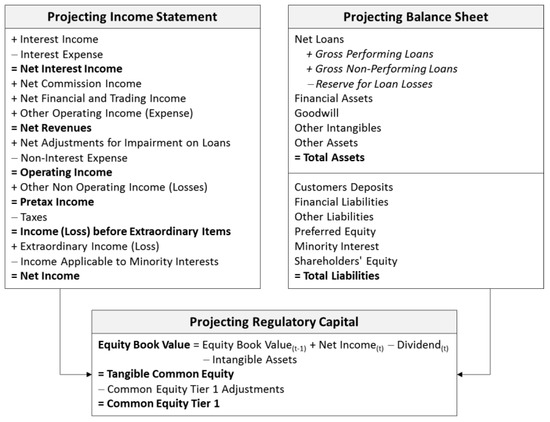
Figure 1.
Projecting Income Statement, Balance Sheet and Regulatory Capital.
The simulations were performed considering fourteen stochastic variables, covering all the main risk factors of a bank. Stochastic variable modeling was done according to a standard setting of rules, which was applied uniformly to all of the banks in the sample. Detailed disclosure on the modeling and all of the assumptions adopted in the exercise is provided in Appendix A. Here below, we briefly describe the general approach adopted to model Pillar I risk factors:
- Credit risk: modeling in through the item loan losses; we adopted the expected loss approach, through which yearly loan loss provisions are estimated as a function of three components: probability of default (PD), loss given default (LGD), and exposure at default (EAD).
- Market risk: modeling in through the item trading and counterparty gains/losses, which includes mark-to market gains/losses, realized and unrealized gains/losses on securities (AFS/HTM) and counterparty default component (the latter is included in market risk because it depends on the same driver as financial assets). The risk factor is expressed in terms of losses/gains rate on financial assets.
- Operational risk: modeling in through the item other non-operating income/losses; this risk factor has been directly modeled, making use of the corresponding regulatory requirement record reported by the banks (considered as maximum losses due to operational risk events); for those banks that did not report any operational risk requirement, we used as proxy the G-SIB sample’s average weight of operational risk over total regulatory requirements.
The exercise includes two sets of simulations of increasing severity: the “Stress[−]” simulation is characterized by a lower severity, while the “Stress[+]” simulation presents a higher severity. Both stress scenarios have been developed in relation to a baseline scenario, used to set the mean values of the distribution functions of the stochastic variables, which for most of the variables, are based on the bank’s historical values. The severity has been scaled by properly setting the variability of the key risk factors, through parameterization of the extreme values of the distribution functions obtained on the basis of the following data set:
- Bank’s track record (latest five years).
- Industry track record, based on a peer group sample made up of 73 banks from different geographic areas comparable with the G-SIB banks.34
- Benchmark risk parameters (PD and LGD) based on Hardy and Schmieder (2013).
For the most relevant stochastic variables, we adopted truncated distribution functions, in order to concentrate the generation of random scenarios within the defined stress test range, restricting samples drawn from the distribution to values between a specified pair of percentiles.
To better illustrate the methodology that is applied for stochastic variable modeling, and in particular, the truncation function process, we report the distributions for some of the main stochastic variables that are related to Credit Agricole in Appendix B.
5. Stress Testing Exercise: Results and Analysis
In this section, we report some of the main results of the stress test exercise that was performed in relation to both Stress[−] and Stress[+] simulations; in addition, we also report in Section 5.1 and Section 5.2, a comparison with the results—disclosed in 2014—of the Federal Reserve/Dodd-Frank act stress test for US G-SIB banks and the EBA/ECB comprehensive assessment stress test for EU G-SIB banks. In Appendix C, a more comprehensive set of records is reported.
The exercise does not represent, to any extent, a valuation of the capital adequacy of the banks considered; stress test results should not be considered as the banks’ expected or most likely figures, but rather should be considered as potential outcomes that are related to the severely adverse scenarios assumed. In the tables, in order to facilitate comparison among the banks that are considered in the analysis, the sample has been clustered into four groups, according to their business model35: IB = Investment Banks; IBU = Investment Banking-Oriented Universal Banks; CB = Commercial Banks; and, CBU = Commercial Banking-Oriented Universal Banks.
The stochastic simulation stress test shows considerable differences in degree of financial fragility among the banks in the sample. These differences are well captured by the CET1 probability of breach records for the three different threshold tested: 8%, 7%, and 4.5%, as reported in Figure 6. For some banks, breach probabilities are very high, while others show very low or even null probabilities. For example, Wells Fargo, ICBC China, Standard Chartered, Bank of China, and State Street show a great resilience to the stress test for all of the years considered and in both Stress[−] and Stress[+] simulations, thanks to their capacity to generate a solid volume of net revenues that are capable of absorbing credit and market losses. Those cases presenting a sharp increase in breach probabilities between Stress[−] and Stress[+] denote relevant non-linear risk conditions in the distribution tail. IB and IBU banks show on average higher probabilities of breach than CB and CBU banks.
Some of the main elements that explain these differences are:
- Current capital base level: banks with higher capital buffers in 2013 came through the stress test better, although this element is not decisive in determining the bank’s fragility ranking.
- Interest income margin: banks with the highest net interest income are the most resilient to the stress test.
- Leverage: banks with the highest leverage are among the most vulnerable to stressed scenarios.36
- Market risk exposures: banks that are characterized by significant financial asset portfolios tend to be more vulnerable to stressed conditions.
In looking at the records, consider that the results were obviously affected by the specific set of assumptions that are adopted in the exercise for the stochastic modeling of many variables. In particular, some of the main risk factor modeling (interest income and expenses, net commissions, credit and market risk) was based on banks’ historical data (the last five years), therefore these records influenced the setting of the distribution functions of the related stochastic variables, with better performance in reducing the function’s variability and extreme negative impacts, and worse performance, increasing the likelihood and magnitude of extreme negative impacts.
The graphs below (Figure 2 and Figure 3) report CET1 ratios and (Figure 4 and Figure 5) report leverage ratio (calculated as: Tangible Common Equity/Net Risk Assets) resulting from the stress test stochastic simulation performed: histograms show first, fifth, and tenth percentiles recorded; last historical (2013). Both of the ratios (CET1 ratios and leverage ratios) are indicated by a green dash, providing a reference point to understand the impact of the stress test; records are shown for 2015 and for both Stress[−] and Stress[+] simulations.
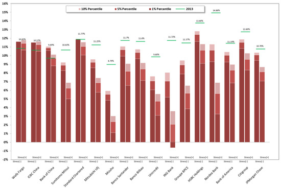
Figure 2.
Stressed CET1 ratio 2015 vs. CET1 ratio 2013. CB & CBU.
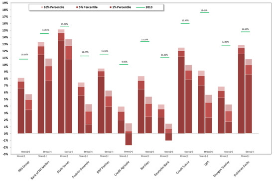
Figure 3.
Stressed CET1 ratio 2015 vs. CET1 ratio 2013. IB & IBU.
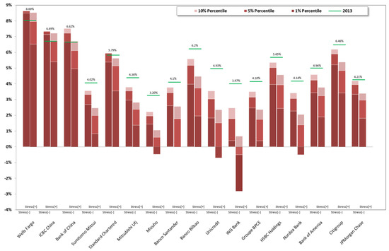
Figure 4.
Stressed leverage ratio 2015 vs. leverage 2013. CB & CBU.
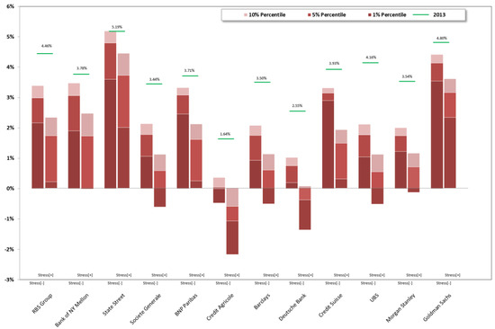
Figure 5.
Stressed leverage ratio 2015 vs. leverage 2013. IB & IBU.
In Figure 6, we report the probability of breach of CET1 ratio for three different thresholds (8%; 7%; 4.5%) in both Stress[−] and Stress[+] simulations.
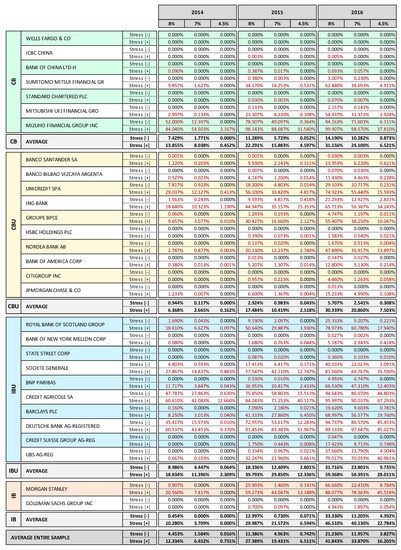
Figure 6.
CET1 ratio probability of breach.
Figure 7 shows the banks’ financial fragility rankings, as provided by the heuristic measure of tail risk (H), determined on the basis of 2015 CET1 ratios. The histograms highlight the range of values determined while considering Stress[−] and Stress[+] simulations. Banks are reported from the most resilient to the most fragile, according to the Stress[+] simulation. The breadth of the range shows the rise in non-linearity conditions in the tail of the distribution due to the increase in the severity of the stress test. The H ranking supports the evidence commented in relation to the previous results.
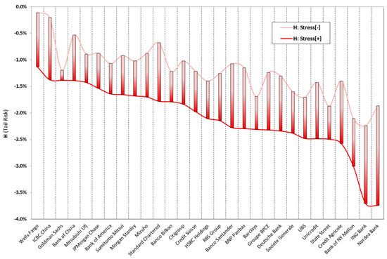
Figure 7.
Heuristic measure of tail risk (CET1 ratio—2015).
5.1. Supervisory Approach to SREP Capital Requirement
The simulation output enables the supervisors to adopt a new forward-looking approach in setting bank-specific minimum capital requirements within the SREP (Supervisory Review and Evaluation Process) process, which can take full advantage of the full depth of the stochastic analysis while insuring an effective level playing field among all of the banks under supervision. The approach would be based on a common minimum capital ratio (trigger of the simulation) and a common level of confidence (probability of breach of the capital ratio in simulation), both set by the supervisors; and, a simulation run by the supervisors. More specifically, supervisors can:
- Set a common predetermined minimum capital ratio “trigger” (α%); of course, this can be done by considering regulatory prescriptions, for example, 4.5% of CET1 ratio, or 7% of CET1 ratio while considering the capital conservation buffer as well.
- Set a common level of confidence “probability threshold” (x%); this probability should be fixed according to the supervisor’s “risk appetite” and also considering the trigger level: the higher the trigger, the lower the probability threshold can be set, since there are higher chances of hitting a high trigger.
- Run a stochastic simulation for each single financial institution with a common standard methodological paradigm.
- Look, for each bank, at the CET1 ratio probability distribution that is generated through the simulation in order to determine the CET1 ratio at the percentile of the distribution that corresponds to the probability threshold (CET1 Ratiox%).
- Compare the value of CET1 Ratiox% to the trigger (α%) in order to see if there is a capital shortfall (−) or excess (+) at that confidence interval (CET1 Ratiox% − α% = ±Δ%); this difference can be transformed into a capital buffer equivalent by multiplying it by the RWA generated in the scenario that corresponds to the percentile threshold (±Δ%·RWAx%).
- Calculate the SREP capital requirement by adding the buffer to the capital position held by the bank at time t0 in the case of capital shortfall at the percentile threshold, or by subtracting the buffer in the case of excess capital; the capital requirement can also be expressed in terms of a ratio by dividing the above capital requirement by the outstanding RWA at t0 or by the leverage exposure if the relevant capital ratio that is considered is the leverage ratio37.
The outlined approach would enable the supervisor to assess in advance the bank-specific capital endowment to be held in order to ensure its adequacy to meet the preset minimum capital ratio at a percentile corresponding to the confidence interval established, throughout the entire time horizon that is considered in the simulation. With a regulatory capital that matches the SREP capital requirement, the bank’s estimated probability of breach of the minimum capital ratio would be equal to the probability threshold and in line with the supervisor risk appetite.
An alternative (to points d, f), simpler way to quantify through the simulative approach the SREP capital requirement entails looking at the probability distribution of economic capital. The economic capital distribution function provides the total cumulated losses that are generated through the simulation at the percentile threshold x%; by adding to that amount the product of the capital ratio trigger and the RWA generated in the percentile threshold scenario (Economic Capitalx% + α%·RWAx%), we obtain a bank’s regulatory capital endowment38 at t0 adequate to cover all of the losses that are estimated through the simulation at the preset confidence interval, while still leaving a capital position that allows for the bank to respect the minimum regulatory capital ratio (trigger)39.
The advantage here is that under a common structured approach for all banks (same probability threshold, regulatory capital trigger, methodological paradigm, etc.), capital requirements could be determined on a bank-specific basis, when considering the impact of all the risk factors that are included in the simulation under an extremely high number of different scenarios, characterized by different levels of severity. This kind of approach is also flexible, allowing for the supervisor, for instance, to address the too big to fail issue in a different way. In fact, rather than setting arbitrary additional capital buffer for G-SII banks, supervisors may assume a lower risk appetite by simply setting a stricter probability threshold for these kinds of institutions (i.e., a higher confidence interval) that are aimed at minimizing their risk of default, and then assessing through a structured simulation process the effective capital endowment that they need to respect the minimum capital ratio at higher confidence intervals.
5.2. Stochastic Simulations Stress Test vs. Fed Supervisory Stress Test
In Figure 8, we report a comparison between the results that were obtained in our stress test exercise and those reported by the Federal Reserve stress test (performed in March 2014) on the US banks of our sample. For the purposes of comparison, we report only results relative to 2015 for both of the stress test exercises. For each bank we report the cumulative losses generated in the stressed conditions simulated distinguished by risk factor and differentiating between gross losses and net losses; gross losses being the stress test impacts associated with the credit and market/counterparty risk factors (i.e., the increase in loans losses provisions and the net financial and trading losses), while net losses are the final net income overall impact of the stress test that affected the capital ratio. The amount of cumulated net losses (Economic Capital) indicates the effective severity of the stress test; conventionally, we indicate with negative Economic Capital figures net losses and with positive Economic Capital figures a net income. We report the stress test total impact also in relative terms with respect to 2013 Net Risk Assets, i.e., the cumulated gross losses on 2013 Net Risk Assets ratio and the net losses on 2013 Net Risk Assets ratio. We also report for each bank RWA and CET1 ratio records. All the records are reported for the two different adverse scenarios that are considered in the Fed stress test (adverse and severely adverse) and for two different confidence intervals (95% and 99%) of the Stress[−] and Stress[+] stochastic simulations performed.
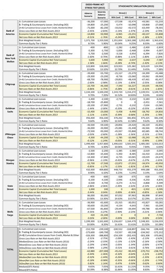
Figure 8.
2015 Stochastic simulation stress test vs. 2015 Federal Reserve stress test. (Data in USD millions/%). (Source of Dodd-Frank Act Stress Test: Federal Reserve 2013a).
Overall, the stochastic simulation stress test exercise provided results that were generally in line with those that were obtained from the Federal Reserve stress test, albeit with some differences. With regard to economic capital, we see that the 99% Stress[−] simulation figures are generally in the range of Fed Adv.–Sev. Adv. scenarios results, while the 99% Stress[+] simulation results show a higher impact than the Fed Sev. Adv. scenario (with the exception of Wells Fargo, which shows very low losses even in extreme scenarios). In the Fed stress test, the range [Adv. 63 bln–Sev. Adv. 207 bln] of the sample’s total amount of economic capital is about the same as the 99th percentile corresponding records range Stress[−] 90 bln–Stress[+] 239 bnl, (see bottom total line Figure 8). It is worth mentioning that while Bank of New York Mellon and State Street reported no losses in the Fed stress test, they show some losses (albeit very low) at the 99th percentile in both Stress[−] and Stress[+] simulations.
Loan losses tend to be quite similar in our exercise to those in the Fed stress test. For some banks (Goldman Sachs, Bank of New York Melon and Morgan Stanley), Stress[+] simulation reported considerably higher impacts than the Fed stress test; this is because we assumed a minimum loss rate in the distribution function that was equal for all banks.
Trading and counterparty losses in our exercise present more differences than in the Fed stress test, due, in part, to the very simplified modeling that is adopted and in part to the role that average historical results on trading income played in our assumptions, which makes the stress less severe for those banks that experienced better trading performances in the recent past (such as Goldman Sachs and Wells Fargo), relative to those that had bad performances (see in particular JPMorgan and Citigroup).
Overall, the median and mean stressed CET1 ratio results of the Fed stress test are in line with those from our stress test exercise, although the Stress[−] simulation shows a slightly lower impact. Also, the total economic capital that is reported in the two stress test exercises are similar, with the total net losses of Fed Adv. Scenario within the range 95–99% of the Stress[−]simulation and the total net losses of Fed Sev. Adv. Scenario within the range 95–99% of the Stress[+] stochastic simulation.
5.3. Stochastic Simulations Stress Test vs. EBA/ECB Supervisory Stress Test
In Figure 9, we report a comparison between the results that were obtained in our stress test exercise and those from the EBA/ECB stress test on the EU banks in our sample—banks that represent more than one-third of the total assets of all the 123 banks that were considered within the supervisory stress test exercise. For the purposes of comparison, we report in Figure 9 only cumulated results for 2016, the last year considered in both exercises.
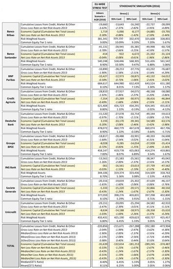
Figure 9.
2016 Stochastic simulation stress test vs. 2016 EBA/ECB comprehensive assessment. (Data in EUR millions/%). (Source of EU-Wide Stress Test: EBA and ECB 2014).
The EBA/ECB stress test results regard the adverse scenario and include the impacts of AQR and join-up and the progressive phasing-in of the more conservative Basel 3 rules for the calculation of CET1 during the 2014–2016 time period of the exercise. These elements contribute to further enhance the adverse impact on CET1 of the EBA/ECB stress test when compared to our simulation, which could not embed the AQR/join-up effects and (being based on 31 December 2013 Basel 2.5 capital ratios) the Basel 3 phasing-in effects. Therefore, the most appropriate way to compare the impact of the two stress tests is to look at the income statement net losses rather than the CET1 drop.
If we look at gross losses, in terms of both average and total values, we can see that the EBA/ECB stress test has a similar impact to Stress[−] simulation, while the Stress[+] simulation shows a notably higher gross impact. It is interesting to note that, when we shift from gross losses to net losses, the EBA/ECB stress test highlights a sharp decrease in its impact, of more than 80%, which effectively reduces the loss rates to very low levels. Looking at individual banks’ results, we can note that, with the exception of Unicredit, all banks have net loss rates well below 1%; in some cases (Banco Bilbao and Deutsche Bank) the overall impact of the stress test and AQR does not determine any net loss at all, but only reduced capital generation. On average, the 95% Stress[−] simulation net loss impact is four times higher than EBA/ECB stress test and the 95% Stress[+] simulation net loss impact is eight times higher. If we compare EBA/ECB to the Fed stress test, notwithstanding the fact that the Fed stress test covers only two years of adverse scenario while EBA/ECB covers three years, we note that, although the Fed stress test reported higher gross losses, impacts are still around the same order of magnitude, 389 billion USD (about 305 billion EUR) of total cumulated gross losses in the Fed stress test with a gross loss rate on net risk assets of 2.75%, against 221 billion EUR total cumulated gross losses in the EBA/ECB stress test with a gross loss rate on net risk assets of 2.04%.40 But, if we look at net losses, we see that in the Fed Sev. Adv. scenario stress test, mitigation in switching to net losses is much lower (−45%, slightly more than the tax effect), 207 billion USD (about 163 billion EUR) of total cumulated net losses with a 1.46% net loss rate, against 36 billion EUR total cumulated net losses in the EBA/ECB stress test with a 0.33% net loss rate, about one-fourth of the Fed net loss rate.
The comparison analysis highlights that the Fed stress test and the stochastic simulation are characterized by a much higher severity than the EBA/ECB stress test, which presents a low effective impact (on average, the 2016 impact is due more to the Basel 3 phasing-in than to the adverse scenario).41 If the EU banks in the sample had all been hit by a net loss rate of 1.5% of net risk assets, equal to the average net loss rate that is recorded in the Fed Sev. Adv. scenario stress test, six of them would not have reached the 5.5% CET1 threshold.42
5.4. Relationship between Stress Test Risk and Market Valuation
With the following analysis, we put bank stress tests results in relation with market value dynamics; the idea is that there should be a certain level of consistency between the effective risk of a bank assessed through a sound forward-looking stress test exercise (performed ex-ante) and the subsequent market evolution of the bank’s stock price. In other words, if the stress testing approach effectively captures the real level of risk, banks with an estimated high risk should be characterized by a lower market appraisal than low risk banks.
We ranked the banks in the sample according to their financial fragility (risk), as measured by their probability of breaching a CET1 ratio threshold of 7% in 2015. The higher the probability of breach, the higher the risk in the ranking. Then, we considered the ratio between market capitalization and tangible assets as a relative synthetic proxy of the market appreciation of the risk embedded in the bank’s assets. We calculated this indicator for each bank at February 2016, about two years after 2013 financial statements (which represent the starting point of all the stress testing exercises) had been made publicly available, a time lapse that we consider long enough for the market to fully incorporate the risk perception that should have been assessed ex-ante with the forward-looking stress test. For a sound stress testing approach, we should expect a negative and significant relation between the riskiness assessed in the 2014 stress test and the subsequent market value dynamic; i.e., the higher the risk assessed through stress testing, the lower the market cap ratio.
Figure 10 reports the results of the correlation analysis between the stochastic simulation stress test and the market cap ratio dynamics; it highlights a significant negative correlation between the stress testing ranking and the market ranking. Each record has also been associated with a color, according to its position in the ranking, ranging from green (low risk) to red (high risk), in order to facilitate the visualization of the matching between the two rankings. Then, we made a similar ranking of the results provided by the two supervisory stress tests. Since probabilities of breach were not estimated in those exercises, we measured the risk in terms of impact of the adverse scenario, i.e., decrease in CET1 ratio during the overall exercise period.
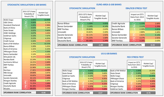
Figure 10.
Stochastic Stress Test Analysis vs. Subsequent Market Dynamic. (Source of Market Data: Bloomberg).
We split the results into two tables in order to compare them among the two groups of banks: Euro area and US. The analysis shows that, also, in the case of the Fed Stress test results, there is a significant negative correlation, while the EBA/ECB stress test shows a positive and non-significant correlation, indicating that the market ex-post had evaluated the level of risk of those banks differently than European supervisors. Of course, from this simple analysis, we cannot draw definitive conclusions, when considering the limited sample size (especially the two sub-samples) and given the fact that the market often fails to appreciate risk and fair value of companies
6. Stochastic Simulation Approach Comparative Back-Testing Analysis
In this section, we tried to obtain some preliminary evidence on the reliability of the stochastic simulation approach in assessing the risk of financial institutions when compared to other methodologies. We first back-tested the proposed approach in assessing the PDs of some famous default cases, when comparing the results with other credit risk assessments. In this case, the model’s quality is quite easy to check, since, for defaulted banks, the interpretation of the back-testing results is straightforward: the model that provides the highest PD estimate earlier in time can be considered that which has the best default predictive power.
Since the ultimate goal of stress testing is to assess banks’ financial fragility, we tried to apply the proposed methodology to three well-known cases of financial distress: Lehman Brothers, Merrill Lynch, and Northern Rock. The aim was to see what kind of insights might have been achieved by assessing the risk of default through the stochastic simulation approach, placing ourselves in a time period preceding the default. Therefore, for each financial institution, we performed two simulations based on the data available at the moment at which they were assumed to have been run. One simulation was set two years before default/bailout (31 January 2007) and based on 2006 financial statement records as the starting point; the other was set about one year before default (3 January 2008) and based on 2007 financial statement.43
We compared the default frequencies estimated through the simulation with other well-known credit risk metrics publicly available at the time and based on different methodologies, namely: PD estimated by Moody’s KMV,44 PD implied in CDS,45 PD implied in the ratings assigned by two rating agencies where available (S&P and Moody’s).46 The analysis is aimed at determining whether the stochastic simulation method might have reported better early warning indications than other credit risk measures. The comparison is made in terms of PDs; all PDs were estimated (where data were available) when considering one-year PD, two-years PD, and three-years PD.
In consideration of the fact that Lehman Brothers and Merrill Lynch at that time were investment banks not subject to banking regulation and therefore did not report regulatory capital ratios, the event of default (the trigger of the stochastic simulation) has been defined as: tangible common equity ≤0. This is a very narrow definition of default, since in the real world a bank would default long before reaching a zero capital level and this must be kept in mind when looking at the results; a simulation run with a broader definition of default (e.g., CET1 ≤ 4.5%) would have highlighted much higher PDs.
We applied the same implementation paradigm that is used for the Stress[+] exercise, as described in Appendix A, with only the following differences, which imply lesser severity overall than in the Stress[+] simulation:
- The market & counterparty risk factor (managed through the net financial and trading income variable) has been modeled according to Appendix A assumptions, but the minimum truncation (max loss rate) for all of the banks has been set at −2.13%, which is half that reported by the G-SIB peer group sample in the latest five years (−4.26%).47
- For Merrill Lynch and Lehman Brothers, the target capital ratio has not been set in terms of risk-weighted capital ratio, since those two financial institutions, being investment banks, did not report such regulatory metrics, but in terms of the leverage ratio (calculated as the ratio between tangible common equity and net fixed assets) reported in the last financial statement available at the moment to which the analysis refers.
- Because of the high interest rate volatility recorded in the years before 2007, in modeling the minimum and maximum parameters of the interest rate distribution functions, we applied only one mean deviation (rather than three, as for Stress[+]).
Figure 11 reports a summary of the results of the back-testing analysis; Appendix D contains the full set of results.
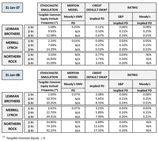
Figure 11.
Default risk comparative back-testing analysis. (Source of CDS, KMV data, rating: Bloomberg, Moody’s KMV, Standard & Poor’s).
For all three banks considered, PDs that are measured by other publicly available models showed very low values in either the 2007 or 2008 analysis. PDs implied in CDS in 2007 did not capture the high risk of default that occurred during the following year; in 2008, they increased significantly, but at that time, all banks experienced a generalized relevant increase in CDS. PDs estimated through the simulative approach (tangible common equity default frequency) show a high level of risk for all banks as early as the 2007 analysis, in particular, with reference to two- and three-year PDs, with a relevant increase in the 2008 analysis.
In looking at the results of the stochastic simulation, we must consider that the baseline initial conditions based on 2006 financial statement records a year in which the banks’ (short term) profitability reached the peak of the speculative bubble (for example, for all three banks, ROE was above 20%). Furthermore, as already mentioned, default frequencies have been determined according to a very narrow definition of the event of default; a common equity trigger higher than zero would have determined much higher default frequencies.
Moreover, it is interesting to note that, for all banks considered, the Funding Shortfall indicator (AFN/equity book value) shows values that are much higher than one48 in extreme percentiles and appreciably higher than the corresponding values that were recorded in the stress test exercise for G-SIB banks (See Appendix D). The high level of AFN/equity book value ratio generated in the worst scenarios and the remarkable increase between 2007 and 2008 simulations, shows that, within the simulation approach, very adverse conditions tends to simultaneously hit capital and liquidity, just as in the real circumstances, in which the default was determined by an abrupt deterioration of both solvency and liquidity conditions. The capacity to capture the solvency-liquidity interlinkage is an important point of strength of the proposed modeling framework.49
Of course, due to the very limited number of cases analyzed, this comparative back-testing analysis cannot be considered as statistically significant; nevertheless, it shows that the stochastic approach proposed, even when being applied in the highly simplified way that we utilized, might have been able to highlight, on the basis of the data available at that time, a high risk that is associated with the three banks, providing a timely early warning that other risk metrics were unable to detect.
7. Conclusions
In our opinion, in assessing a bank’s financial fragility we need not try to forecast specific exceptional adverse events and calculate the corresponding losses, nor is it necessary to adopt an overly complex and analytically detailed modeling apparatus, which, in the attempt to ensure a presumed “high fidelity” in terms of calculation accuracy, ends up disregarding some of the most relevant phenomena for assessing a bank’s resilience. In this regard, it is worth recalling what Andrew G. Haldane stressed: “(…) all models are wrong. The only model that is not wrong is reality and reality is not, by definition, a model. But, risk management models have during this crisis proven themselves wrong in a more fundamental sense. They failed Keynes’ test—that it is better to be roughly right than precisely wrong. With hindsight, these models were both very precise and very wrong.”50 In that sense, our aim in this paper is to present a “roughly right” methodological approach for stress-testing analysis aimed at evaluating a bank’s financial fragility and its general resiliency capacity.
We have tried to show how the proposed methodology overcomes some of the limitations of current mainstream stress testing approaches, presenting a new approach that is less laborious and time-consuming, yet at the same time, allows for a deeper analysis, by largely expand the number of adverse scenarios considered and by integrating all the solvency and liquidity risk factors within a single consistent framework. The empirical exercise we describe shows how even with an extremely simplified modeling and application of the approach, a comprehensive and meaningful stress test can be realized.
The flexibility of the approach allows for different levels of complexity/analyticity, depending on data set availability and the purpose of the analysis. This makes it well suited both for internal bank use in risk appetite and capital adequacy processes, and by analysts and supervisory authorities, for external risk assessment purposes.
Supervisors should perform stress test exercises themselves, avoiding reliance on banks’ internal models (bottom up approach) for the calculation of losses, so as to speed up and simplify the process, ensure an effective comparability of results across institutions on a level playing field and avoid any moral hazard issues. The handiness of the top down approach described allows for them to do so, keeping the analysis time and effort that is required at a reasonable level.
Furthermore, the stochastic approach proposed leads the way to a new bank specific approach for setting SREP capital requirements, based on a common interval of confidence, a common minimum capital ratio threshold, and a common standard quantitative modeling; thus, ensuring an effective level playing field in the SREP risk to capital assessment.
In conclusion, the most relevant advantage of the simulative methodology that we propose is that by considering the impacts that are related to an extremely high number of potential different adverse future scenarios, it generates results expressed in probabilistic terms. This allows for us to evaluate more efficaciously and in advance the overall riskiness of a bank within a more comprehensive framework, thus making stress testing a truly effective tool in assessing banks’ financial fragility and supporting timely capital adequacy decisions.
Author Contributions
Both authors contributed to the development of all the parts of the article, therefore there are no specific contributions or attributions.
Funding
This research received no external funding.
Acknowledgments
Our special thanks to Antonio Dicanio, Donato Di Martino, Claudia Franchi and Luigi Ronga for their precious collaboration in the development of the empirical analysis.
Conflicts of Interest
The authors declare no conflict of interest.
Appendix A. Main Assumptions Adopted in the Stress Test Exercise
The stress test exercise performed has been developed exclusively as an exemplification for illustrative purposes and does not represent to any extent a valuation on the capital adequacy of the banks considered. Therefore, the assumptions described here below are intended solely for this explanatory aim, must be considered as only one possible sensible set of assumptions and do not by any means represent the only or the best implementation paradigm of the stochastic simulation model proposed. For stress tests that more efficaciously measure financial fragility and default risk, more evolved implementation paradigms can easily be adopted, using a broader and more accurate set of data if available.
Number of Scenarios Simulated: For each simulation 30,000 trials were generated.
Stochastic Variable Distribution Functions: The figure below reports the assumptions adopted for modeling the stochastic variable distribution functions. For many variables we adopted a standard symmetric distribution modeled through Beta functions, with shape parameters (4, 4), in order to have a definite domain of the functions. The modeling of variables made are through other asymmetric functions is based on statistical analysis performed on the peer group sample or standard literature modeling (i.e., PD). Some distribution functions were truncated (through a standard truncation approach) in order to focus the simulation within a stressed range of values.
For each stochastic variable we report the kind of function, the Native Distribution Parameter Setting, the method used for the parameter estimate, and the Truncated Distribution Parameter Setting method (for those variables for which truncation function has been applied).
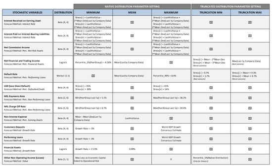
Figure A1.
Stochastic variables: modeling & assumptions.
Credit Risk Modeling:51 The defaulted credit flow in each period is determined as the product of the expected default rate (PD) at the end of the period times the value of performing loans at the beginning of the period, thus assuming that the new loans do not default during the period in which they have been granted:
The NPL stock is determined as:
where w is the write-off rate, r the payment rate and b the NPL cure rate (recovery of exposures from NPL to performing loans). Thus the “net adjustments for impairment on loans” is determined as:
where LGD is the loss given default, which for the sake of simplicity is assumed equal for performing and non-performing loans.52 The first addendum represents the impairments on new defaulted loans; the second addendum represents the impairments on old defaulted loans due to a change in the coverage of NPLs that occurs any time that occurs ; the third addendum represents the release of provisions accumulated in the Reserve for Loan Losses, caused by a migration of some NPLs back to a performing status and are determined according to the LGD of the previous period.
The loan losses reserve at the end of the period is then given by the reserve at the beginning of the period, plus the net adjustments for impairment on loans, less the part of the reserve related to loans written off during the period:53
Assuming that performing loans grow with a rate equal to g, we have:
and so, the stock of performing loans at the end of each period is given by:
Interest income is determined on the basis of the average stock of gross performing loans, assuming that all NPLs do not earn any interest income. Net loans are then determined as:
The five variables: PD, LGD, w, r, g, are considered as stochastic variables and their distribution functions are modeled according to the rules indicate in the figure above. For the sake of simplicity, the cure rate b is set equal to zero.
Default Rate: To model default rate as a stochastic variable we used bank-specific data and benchmark stressed parameters reported by Hardy and Schmieder (2013):

Table A1.
Stress levels of default rates and LGDs for advance countries.
Table A1.
Stress levels of default rates and LGDs for advance countries.
| Scenario | Normal | Moderate | Medium | Severe | Extreme |
|---|---|---|---|---|---|
| Default Rates/1 | 0.7% | 1.7% | 2.9% | 5% | 8.4% |
| Projected LGD | 26% | 30% | 34% | 41% | 54% |
Source: Hardy and Schmieder (2013, p. 21).
Since PD values were not available, to model default rates we adopted a rough proxy based on the only publicly available data common to all banks. Default rates are given by the ratio between defaulted credit flow at the end of the period and gross performing loans at the beginning of the period. Since we do not have data for defaulted credit flow but only for NPL stock, we tried to obtain a proxy of defaulted credit flow by dividing NPLs by the estimated average time taken to generate the current stock of NPLs (NPL Generation Time), which we assumed to be equal to the number of years necessary to accumulate the reserve for loan losses, that we calculated as the ratio between Reserve for Loan Losses and the average impairment flow in the last five years, through the following formula:
Thus, the default rate [PD] is given by:
Of course, we are well aware that the default rate estimated using the procedure outlined above is a rough estimate of the real historical data, but it is the best simple proxy measure we were able to work out given the limited data set available; the use of more accurate records would certainly improve the meaningfulness of the results.
To define the distribution function of default rate we proceeded as follows:
- We adopted a Weibull function (1, 5) characterized by right tail; this is a typical widespread modeling of the default rate distribution.
- We defined the native distribution function by setting the mean and maximum parameters; for the entire stress test time horizon the mean is given for each bank by the average of default rate estimates from the last 5 years, and the maximum is set for all banks at 8.4%, which corresponds to the default rate associated in advanced countries with an extremely severe adverse scenario in Hardy and Schmieder benchmarks.
- We truncated the native function. The minimum truncation has been set for all banks at 0.7% in the Stress[−] simulation, which corresponds to a “normal” scenario in Hardy and Schmieder benchmarks; and to 1.7% in the Stress[+] simulation, which corresponds to a “moderately” adverse scenario in Hardy and Schmieder benchmarks. The maximum truncation has been determined for each bank by adding to the bank’s mean value of the native function a stress impact determined on the basis of the benchmark default rate increase realized by switching to a more adverse scenario. This method of modeling default rate extreme values allows us to calibrate the distribution function according to the specific bank’s risk level (i.e., banks with a higher average default rate have a higher maximum truncated default rate). Therefore, to determine the maximum truncation in the Stress[−] simulation we added to the bank’s mean the difference between the “severe” scenario (5%) and the “normal” scenario (0.7%) from Hardy and Schmieder benchmarks, or:
In the Stress[+] simulation we added to the bank’s mean the difference between the “extreme” scenario (8.4%) and the “moderate” scenario (1.7%) of Hardy and Schmieder benchmarks, or:
For an example of the truncation process of PD distribution function see Appendix B.
LGD (Loss Given Default): LGD distribution functions have been modeled using Hardy and Schmieder benchmarks (see Table A1) in the following way:
- We adopted a symmetrical Beta function (4, 4).
- We defined the distribution function by setting the minimum and maximum parameters; for the entire stress test time horizon and for all banks, in the Stress[−] simulation we set the minimum at 26%, which corresponds to the LGD benchmark associated in advanced countries (see Table A1) with a normal scenario; the maximum is set to 41%, which corresponds to the LGD benchmarks associated in advanced countries with a severe adverse scenario. In the Stress[+] simulation we set the minimum to 30%, which corresponds to the LGD benchmarks associated in advanced countries with a moderate scenario; the maximum is set to 54%, which corresponds to the LGD benchmarks associated in advanced countries with a extreme adverse scenario.
NPLs Write-off and Payment Rate: The distribution functions of the NPLs write-off rate and NPLs payments rate are both defined by setting the minimum and maximum parameters; these parameters are set for all banks equal to the corresponding minimum and maximum recorded within a sample of G-SIB peer banks.
Market and Counterparty Risk: We model market risk and counterparty risk jointly since they are both connected to the stock of financial assets. These risk factors are managed through the “Net Financial and Trading Income” variable, determined as rate of return on the stock of financial assets. The stochastic variable has been modeled through a logistic function; which was estimated through an empirical statistical analysis based on the banks’ peer group sample indicated in Section 4. The distribution function is defined by its minimum and mean parameters held constant through the entire forecast time period; the mean has been set for each bank according to its average value from the latest five years’ records, and the minimum54 has been set for all banks at −4.26%, representing the first percentile of records within a bank peer group sample from the last 5 years. The distribution function has been truncated; the minimum truncation has been determined as the difference between the mean of the native function and mean deviations determined within the bank peer group sample, we considered 2 mean deviations in Stress[−] and 3 mean deviations in Stress[+]. The maximum truncation has been set for each bank according to its best record over the last 5 years. For an example of the truncation process of Net Financial and Trading Income distribution function see Appendix B.
Risk Weighted Assets: Risk Weighted Assets have been determined as risk weighted factors or [RW = Risk Weighted Assets/Net Risk Asset] and modeled through a Beta function (4, 4) defined by setting its minimum and maximum parameters. It is assumed that the min/max range will grow according to an exponential stochastic pattern, starting in 2014 with the following min/max values:
And ending in 2016 with the following min/max values:
where is given by the latest risk weighted factor available and ΔRW represents the increase in the risk weighted factor and is obtained through the following function:
Dividend/Capital Retention Policy: Dividend payments and capital retention are determined endogenously by the forecasting model through the rules indicated in Section 3, and thus depend on the target capital ratio (the higher the target capital ratio, the higher the capital retention rate during the simulation time horizon). To set the target capital ratio, we consider an indicative threshold of 12%, given by a comprehensive G-SIB Basel III threshold for common equity tier 1 including: minimum requirement 4.5%; capital conservation buffer 2.5%; maximum countercyclical capital buffer 2.5%; maximum G-SIB capital buffer 2.5%. For all those banks that reported in their latest financial statement (2013) a capital ratio higher than 12%, we set the target ratio equal to the latest record reported and held it constant through the entire forecast period; for those banks that reported in their latest financial statement (2013) a capital ratio lower than 12%, we set the target ratio equal to the latest record reported and increased it linearly up to 12% during the three forecast periods.
Deterministic Variables: All other non-stochastic variables have been assumed as equal to the corresponding value reported in the latest financial statement record (2013), with the exception of financial liabilities, which are determined endogenously by the forecasting model on the basis of the rules indicated in Section 3. The Figure A2 below reports the assumptions adopted.
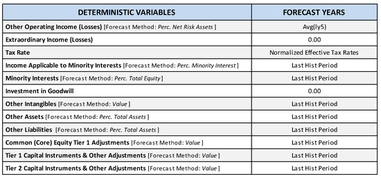
Figure A2.
Deterministic variables: modeling & assumptions.
Correlation Matrix: The Figure A3 below shows the Correlation Matrix assumptions adopted. Most of the correlation coefficients are based on historical cross-section empirical analysis, derived from 2007–2012 data, a period characterized by severe stress for the banking industry (Spearman Rank Correlation has been used as correlation measure). The remaining correlation coefficients have been set according to theoretical assumptions aimed at replicating interdependence relationships under stress conditions. The qualitative classification reported in the boxes adopts the following conventional values: very large = 0.7, large = 0.5, medium = 0.3, small = 0.2.55
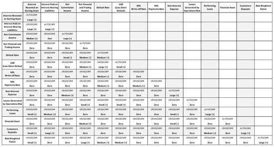
Figure A3.
Correlations assumptions.
Data Source and Processing: Bloomberg: historical financial statement data, consensus forecast on GDP. Banks’ financial statement report (Pillar 3 section): regulatory requirement data set. Data elaboration and stochastic simulations have been processed by value.Bank, software application available on Bloomberg terminal (APPS VBANK <GO>).
Appendix B. Stochastic Variables Modeling (Credit Agricole)
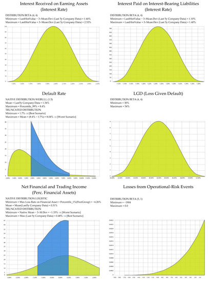
Figure A4.
Probability distribution functions of key stochastic variables for Credit Agricole simulation.
Appendix C. Stochastic Simulation Stress Test Analytical Results
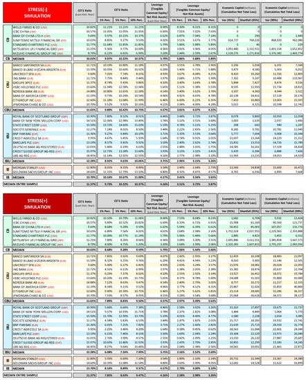
Figure A5.
2014 Stress test exercise: capital adequacy and economic capital.
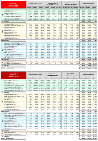
Figure A6.
2014 Stress test exercise: credit/market cumulative losses and funding shortfall.
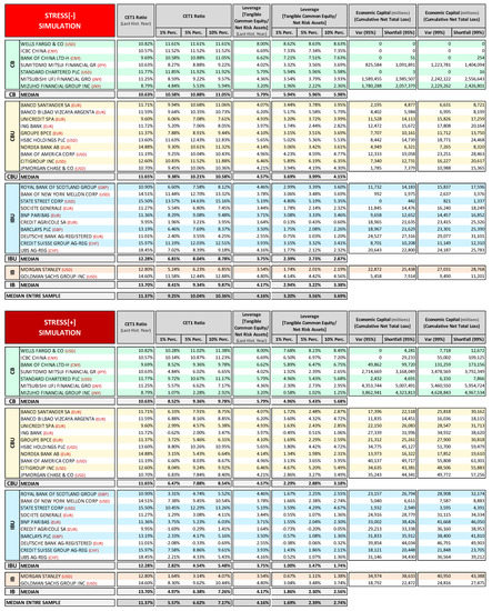
Figure A7.
2015 Stress test exercise: capital adequacy and economic capital.
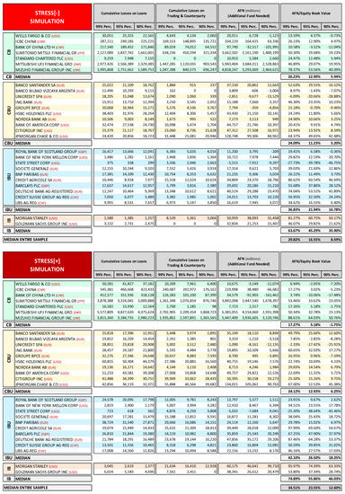
Figure A8.
2015 Stress test exercise: credit/market cumulative losses and funding shortfall.
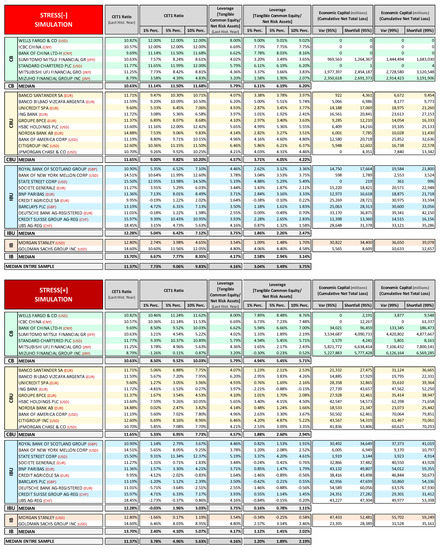
Figure A9.
2016 Stress test exercise: capital adequacy and economic capital.
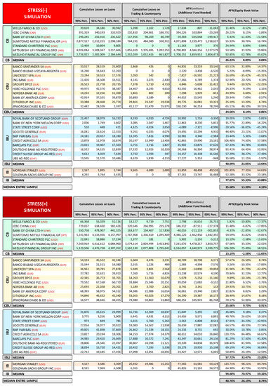
Figure A10.
2016 Stress test exercise: credit/market cumulative losses and funding shortfall.
Appendix D. Back-Testing Analysis Results
This Appendix reports the complete set of results obtained within the comparative back-testing analysis. For each bank the first section of records reports the comparison among the different PD estimates; PDs refer to different time horizons: 1-year PD, 2-years PD and 3-years PD. The lower section reports the potential losses (economic capital) and some additional indicators estimated through the stochastic simulation within the three years of projections considered.
The records reported correspond to the most extreme percentiles of their distribution functions, 1% and 5% for leverage and CET1 ratio (the latter is available only for Northern Rock); and 95% and 99% for economic capital (cumulated losses) and Funding Shortfall (calculated as AFN/equity book value of the latest financial statement available).
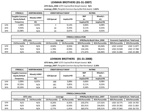
Figure A11.
Backtesting comparative analysis: Lehman Brothers. (Source of CDS, KMV data, rating: Bloomberg, Moody’s KMV, Standard & Poor’s).
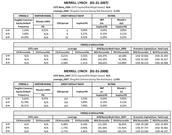
Figure A12.
Backtesting comparative analysis: Merrill Lynch. (Source of CDS, KMV data, rating: Bloomberg, Moody’s KMV, Standard & Poor’s).
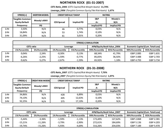
Figure A13.
Backtesting comparative analysis: Northern Rock. (Source of CDS, KMV data, rating: Bloomberg, Moody’s KMV, Standard & Poor’s).
References
- Admati, Anat R., and Martin Hellwig. 2013. The Bankers’ New Clothes: What’s Wrong with Banking and What to Do about It. Princeton: Princeton University Press. [Google Scholar]
- Admati, Anat R., Franklin Allen, Richard Brealey, Michael Brennan, Markus K. Brunnermeier, Arnoud Boot, John H. Cochrane, Peter M. DeMarzo, Eugene F. Fama, Michael Fishman, and et al. 2010. Healthy Banking System is the Goal, not Profitable Banks. Financial Times, November 9. [Google Scholar]
- Admati, Anat R., Peter M. DeMarzo, Martin F. Hellwig, and Paul C. Pfleiderer. 2016. Fallacies, Irrelevant Facts, and Myths in the Discussion of Capital Regulation: Why Bank Equity Is Not Expensive. Available online: https://dx.doi.org/10.2139/ssrn.2349739 (accessed on 14 August 2018).
- Alfaro, Rodrigo, and Mathias Drehmann. 2009. Macro stress tests and crises: What can we learn? BIS Quarterly Review. December 7, pp. 29–41. Available online: https://www.bis.org/publ/qtrpdf/r_qt0912e.htm (accessed on 14 August 2018).
- Bank of England. 2013. A Framework for Stress Testing the UK Banking System: A Discussion Paper. London: Bank of England, October. [Google Scholar]
- Basel Committee on Banking Supervision. 2009. Principles for Sound Stress Testing Practices and Supervision. No. 155. Basel: Bank for International Settlements, March 13. [Google Scholar]
- Berkowitz, Jeremy. 1999. A coherent framework for stress-testing. Journal of Risk 2: 5–15. [Google Scholar] [CrossRef]
- Bernanke, Ben S. 2013. Stress Testing Banks: What Have We Learned? Paper presented at the "Maintaining Financial Stability: Holding a Tiger by the Tail" Financial Markets Conference, Georgia, GA, USA, April 8. [Google Scholar]
- Borio, Claudio, Mathias Drehmann, and Kostas Tsatsaronis. 2012a. Stress-testing macro stress testing: Does it live up to expectations? Journal of Financial Stability 42: 3–15. [Google Scholar] [CrossRef]
- Borio, Claudio, Mathias Drehmann, and Kostas Tsatsaronis. 2012b. Characterising the financial cycle: Don’t lose sight of the medium term! Social Science Electronic Publishing 68: 1–18. [Google Scholar]
- Carhill, Michael, and Jonathan Jones. 2013. Stress-Test Modelling for Loan Losses and Reserves. In Stress Testing: Approaches, Methods and Applications. Edited by Siddique Akhtar and Iftekhar Hasan. London: Risk Books. [Google Scholar]
- Cario, Marne C., and Barry L. Nelson. 1997. Modeling and Generating Random Vectors with Arbitrary Marginal Distributions and Correlation Matrix. Evanston: Northwestern University. [Google Scholar]
- Cecchetti, Stephen G. 2010. Financial Reform: A Progress Report. Paper presented at the Westminster Economic Forum, National Institute of Economic and Social Research, London, UK, October 4. [Google Scholar]
- Čihák, Martin. 2004. Stress Testing: A Review of Key Concepts. Prague: Czech National Bank. [Google Scholar]
- Čihák, Martin. 2007. Introduction to Applied Stress Testing. IMF Working Papers 07. Washington, DC: International Monetary Fund. [Google Scholar] [CrossRef]
- Clemen, Robert T., and Terence Reilly. 1999. Correlations and copulas for decision and risk analysis. Management Science 45: 208–24. [Google Scholar] [CrossRef]
- Cohen, Jacob. 1988. Statistical Power Analysis for the Behavioral Sciences, 2nd ed. Hillsdale: Lawrence Erlbaum Associates. [Google Scholar]
- Demirguc-Kunt, Asli, Enrica Detragiache, and Ouarda Merrouche. 2013. Bank capital: Lessons from the financial crisis. Journal of Money Credit & Banking 45: 1147–64. [Google Scholar]
- Drehmann, Mathias. 2008. Stress tests: Objectives challenges and modelling choices. Sveriges Riskbank Economic Review 2008: 60–92. [Google Scholar]
- European Banking Authority (EBA). 2011a. Overview of the EBA 2011 Banking EU-Wide Stress Test. London: European Banking Authority. [Google Scholar]
- European Banking Authority (EBA). 2011b. Overview of the 2011 EU-Wide Stress Test: Methodological Note. London: European Banking Authority. [Google Scholar]
- European Banking Authority (EBA). 2013a. Report on the Comparability of Supervisory Rules and Practices. London: European Banking Authority. [Google Scholar]
- European Banking Authority (EBA). 2013b. Third Interim Report on the Consistency of Risk-Weighted Assets—SME and Residential Mortgages. London: European Banking Authority. [Google Scholar]
- European Banking Authority (EBA). 2013c. Report on Variability of Risk Weighted Assets for Market Risk Portfolios. London: European Banking Authority. [Google Scholar]
- European Banking Authority (EBA). 2014a. Fourth Report on the Consistency of Risk Weighted Assets-Residential Mortgages Drill-Down Analysis. London: European Banking Authority. [Google Scholar]
- European Banking Authority (EBA). 2014b. Methodology EU-Wide Stress Test 2014. London: European Banking Authority. [Google Scholar]
- Embrechts, Paul, Alexander McNeil, and Er Mcneil Daniel Straumann. 1999. Correlation: pitfalls and alternatives. Risk Magazine 1999: 69–71. [Google Scholar]
- Estrella, Arturo, Sangkyun Park, and Stavros Peristiani. 2000. Capital ratios as predictors of bank failure. Economic Policy Review 86: 33–52. [Google Scholar]
- Federal Reserve. 2012. Comprehensive Capital Analysis and Review 2012: Methodology for Stress Scenario Projection; Washington, DC: Federal Reserve.
- Federal Reserve. 2013a. Dodd-Frank Act Stress Test 2013: Supervisory Stress Test Methodology and Results; Washington, DC: Federal Reserve.
- Federal Reserve. 2013b. Capital Planning at Large Bank Holding Companies: Supervisory Expectations and Range of Current Practice; Washington, DC: Federal Reserve.
- Federal Reserve. 2014. Dodd–Frank Act Stress Test 2014: Supervisory Stress Test Methodology and Results; Washington, DC: Federal Reserve.
- Federal Reserve, Federal Deposit Insurance Corporation (FDIC), and Office of the Comptroller of the Currency (OCC). 2012. Guidance on Stress Testing for Banking Organizations with Total Consolidated Assets of More Than $10 Billion; Washington, DC: Federal Reserve, Washington, DC: Federal Deposit Insurance Corporation, Washington, DC: Office of the Comptroller of the Currency.
- Ferson, Scott, Janos Hajagos, Daniel Berleant, Jianzhong Zhang, W. Troy Tucker, Lev Ginzburg, and William Oberkampf. 2004. Dependence in Probabilistic Modeling, Dempster-Shafer Theory, and Probability Bounds Analysis; SAND2004-3072. Albuquerque: Sandia National Laboratories.
- Foglia, Antonella. 2009. Stress testing credit risk: A survey of authorities’ approaches. International Journal of Central Banking 5: 9–42. [Google Scholar] [CrossRef]
- Financial Stability Board (FSB). 2013. 2013 Update of Group of Global Systemically Important Banks (G-SIBs). Basel: Financial Stability Board. [Google Scholar]
- Gambacorta, Leonardo, and Adrian van Rixtel. 2013. Structural Bank Regulation Initiatives: Approaches and Implications. No. 412. Basel: Bank for International Settlements. [Google Scholar]
- Geršl, Adam, Petr Jakubík, Tomas Konečný, and Jakub Seidler. 2012. Dynamic stress testing: The framework for testing banking sector resilience used by the Czech National Bank. Czech Journal of Economics and Finance 63: 505–36. [Google Scholar]
- Greenlaw, David, Anil K. Kashyap, Kermit Schoenholtz, and Hyun Song Shin. 2012. Stressed Out: Macroprudential Principles for Stress Testing. No. 71. Chicago: The University of Chicago Booth School of Business. [Google Scholar]
- Guegan, Dominique, and Bertrand K. Hassani. 2014. Stress Testing Engineering: the Real Risk Measurement? In Future Perspectives in Risk Models and Finance. Edited by Alain Bensoussan, Dominique Guegan and Charles S. Tapiero. Cham: Springer International Publishing, pp. 89–124. [Google Scholar]
- Haldane, Andrew G., and Vasileios Madouros. 2012. The dog and the frisbee. Economic Policy Symposium-Jackson Hole 14: 13–56. [Google Scholar]
- Haldane, Andrew G. 2009. Why Banks Failed the Stress Test. Paper presented at The Marcus-Evans Conference on Stress-Testing, London, UK, February 9–10. [Google Scholar]
- Hardy, Daniel. C., and Christian Schmieder. 2013. Rules of Thumb for Bank Solvency Stress Testing. No. 13/232. Washington, DC: International Monetary Fund. [Google Scholar]
- Henry, Jerome, and Christoffer Kok. 2013. A Macro Stress Testing Framework for Assessing Systemic Risks in the Banking Sector. No. 152. Frankfurt: European Central Bank. [Google Scholar]
- Hirtle, Beverly, Anna Kovner, James Vickery, and Meru Bhanot. 2016. Assessing financial stability: The capital and loss assessment under stress scenarios (CLASS) model. Journal of Banking & Finance 69: S35–S55. [Google Scholar] [CrossRef]
- International Monetary Fund (IMF). 2012. Macrofinancial Stress Testing: Principles and Practices. Washington, DC: International Monetary Fund, August 22. [Google Scholar]
- Jagtiani, Julapa, James Kolari, Catharine Lemieux, and Hwan Shin. 2000. Early Warning Models for Bank Supervision: Simpler Could Be Better. Chicago: Federal Reserve Bank of Chicago. [Google Scholar]
- Jobst, Andreas A., Li L Ong, and Christian Schmieder. 2013. A Framework for Macroprudential Bank Solvency Stress Testing: Application to S-25 and Other G-20 Country FSAPs. No. 13/68. Washington, DC: International Monetary Fund. [Google Scholar]
- Kindleberger, Charles P. 1989. Manias, Panics, and Crashes: A History of Financial Crises. New York: Basic Books. [Google Scholar]
- Le Leslé, Vanessa, and Sofiya Avramova. 2012. Revisiting Risk-Weighted Assets: Why Do RWAs Differ across Countries and What Can Be Done about It? No. 12/90. Washington, DC: International Monetary Fund. [Google Scholar]
- Martel, Manuel Merck, Adrian van Rixtel, and Emiliano Gonzalez Mota. 2012. Business Models of International Banks in the Wake of the 2007–2009 Global Financial Crisis. No. 22. Madrid: Bank of Spain, pp. 99–121. [Google Scholar]
- Merton, Robert C. 1974. On the pricing of corporate debt: The risk structure of interest rates. Journal of Finance 29: 449–70. [Google Scholar]
- Minsky, Hyman P. 1972. Financial Instability Revisited: The Economics of Disaster; Washington, DC: Federal Reserve, vol. 3, pp. 95–136.
- Minsky, Hyman P. 1977. Banking and a fragile financial environment. The Journal of Portfolio Management Summer 3: 16–22. [Google Scholar] [CrossRef]
- Minsky, Hyman P. 1982. Can It Happen Again? Essay on Instability and Finance. Armonk: M. E. Sharpe. [Google Scholar]
- Minsky, Hyman P. 2008. Stabilizing an Unstable Economy. New York: McGraw Hill. [Google Scholar]
- Montesi, Giuseppe, and Giovanni Papiro. 2014. Risk analysis probability of default: A stochastic simulation model. Journal of Credit Risk 10: 29–86. [Google Scholar] [CrossRef]
- Nelsen, Roger B. 2006. An Introduction to Copulas. New York: Springer. [Google Scholar]
- Puhr, Claus, and Stefan W. Schmitz. 2014. A view from the top: The interaction between solvency and liquidity stress. Journal of Risk Management in Financial Institutions 7: 38–51. [Google Scholar]
- Quagliariello, Mario. 2009a. Stress-Testing the Banking System: Methodologies and Applications. Cambridge: Cambridge University Press. [Google Scholar]
- Quagliariello, Mario. 2009b. Macroeconomic Stress-Testing: Definitions and Main Components. In Stress-Testing the Banking System: Methodologies and Applications. Edited by Mario Quagliariello. Cambridge: Cambridge University Press. [Google Scholar]
- Rebonato, Riccardo. 2010. Coherent Stress Testing: A Bayesian Approach to the Analysis of Financial Stress. Hoboken: Wiley. [Google Scholar]
- Robert, Christian P., and George Casella. 2004. Monte Carlo Statistical Methods, 2nd ed. New York: Springer. [Google Scholar]
- Rubinstein, Reuven Y. 1981. Simulation and the Monte Carlo Method. New York: John Wiley & Sons. [Google Scholar]
- Schmieder, Christian, Maher Hasan, and Claus Puhr. 2011. Next Generation Balance Sheet Stress Testing. No. 11/83. Washington, DC: International Monetary Fund. [Google Scholar]
- Schmieder, Christian, Heiko Hesse, Benjamin Neudorfer, Claus Puhr, and Stefan W. Schmitz. 2012. Next Generation System-Wide Liquidity Stress Testing. No. 12/03. Washington, DC: International Monetary Fund. [Google Scholar]
- Siddique, Akhtar, and Iftekhar Hasan. 2013. Stress Testing: Approaches, Methods and Applications. London: Risk Books. [Google Scholar]
- Taleb, Nassim N., and Raphael Douady. 2013. Mathematical definition, mapping, and detection of (anti)fragility. Quantitative Finance 13: 1677–89. [Google Scholar] [CrossRef]
- Taleb, Nassim N. 2011. A Map and Simple Heuristic to Detect Fragility, Antifragility, and Model Error. Available online: http://www.fooledbyrandomness.com/heuristic.pdf (accessed on 14 August 2018).
- Taleb, Nassim N. 2012. Antifragile: Things That Gain from Disorder. New York: Random House. [Google Scholar]
- Taleb, Nassim N., Elie Canetti, Tediane Kinda, Elena Loukoianova, and Christian Schmieder. 2012. A New Heuristic Measure of Fragility and Tail Risks: Application to Stress Testing. No. 12/216. Washington, DC: International Monetary Fund. [Google Scholar]
- Tarullo, Daniel K. 2014a. Rethinking the Aims of Prudential Regulation. Paper presented at The Federal Reserve Bank of Chicago Bank Structure Conference, Chicago, IL, USA, May 8. [Google Scholar]
- Tarullo, Daniel K. 2014b. Stress Testing after Five Years. Paper presented at The Federal Reserve Third Annual Stress Test Modeling Symposium, Boston, MA, USA, June 25. [Google Scholar]
- Zhang, Jing. 2013. CCAR and Beyond: Capital Assessment, Stress Testing and Applications. London: Risk Books. [Google Scholar]
| 1 | As highlighted by Taleb (2012, pp. 4–5): “It is far easier to figure out if something is fragile than to predict the occurrence of an event that may harm it. [...] Sensitivity to harm from volatility is tractable, more so than forecasting the event that would cause the harm.” |
| 2 | See Montesi and Papiro (2014). |
| 3 | Guegan and Hassani (2014) propose a stress testing approach, in a multivariate context, that presents some similarities with the methodology outlined in this work. Also, Rebonato (2010) highlights the importance of applying a probabilistic framework to stress testing and presents an approach with similarities to ours. |
| 4 | The topic is covered extensively in the literature. For a survey of stress testing technicalities and approaches see (Berkowitz 1999; Čihák 2004, 2007; Drehmann 2008; Basel Committee on Banking Supervision 2009; Quagliariello 2009a, 2009b; Schmieder et al. 2011; Geršl et al. 2012; Greenlaw et al. 2012; IMF 2012; Siddique and Hasan 2013; Jobst et al. 2013; Henry and Kok 2013; Zhang 2013; Hirtle et al. 2016). For technical documentation, methodology and comments on supervisory stress testing see (Haldane 2009; EBA 2011a, 2011b, 2014b; Federal Reserve/FDIC/OCC 2012; Federal Reserve 2012, 2013a, 2013b, 2014; Bernanke 2013; Bank of England 2013; Tarullo 2014b). |
| 5 | Here the term “speculative position” is to be interpreted according to Minsky’s technical meaning, i.e., a position in which an economic agent needs new borrowing in order to repay outstanding debt. |
| 6 | Berkowitz (1999). At this regard see also Rebonato (2010, pp. 1–13). |
| 7 | See in particular Minsky (1982, 2008) and Kindleberger (1989) contributions on financial instability. |
| 8 | At this regard see Alfaro and Drehmann (2009), Borio et al. (2012a, 2012b). |
| 9 | “If communication is the main objective for a Financial Stability stress test, unobservable factors may not be the first modelling choice as they are unsuited for storytelling. In contrast, using general equilibrium structural macroeconomic models to forecast the impact of shocks on credit risk may be very good in highlighting the key macroeconomic transmission channels. However, macro models are often computationally very cumbersome. As they are designed as tools to support monetary policy decisions they are also often too complex for stress testing purposes”. Drehmann (2008, p. 72). |
| 10 | In this regard the estimate of intra-risk diversification effect is a relevant issue, especially in tail events, for which it is incorrect to simply add up the impacts of the different risk factors estimated separately. For example, consider that for some risk measures, such as VaR, the subadditivity principle is valid only for elliptical distributions (see for example Embrechts et al. 1999). As highlighted by Quagliariello (2009b, p. 34): “ … the methodologies for the integration of different risks are still at an embryonic stage and they represent one of the main challenges ahead.” |
| 11 | Such a model may also in principle be able to capture the capital impact of strategic and/or reputational risk, events that have an impact essentially through adverse dynamics of interest income/expenses, deposits, non-interest income/expenses. |
| 12 | See Haldane (2009, pp. 6–7). |
| 13 | In this regard, Bernanke (2013, pp. 8–9) also underscores the importance of an independent Federal Reserve management and the running of stress tests: “These ongoing efforts are bringing us close to the point at which we will be able to estimate, in a fully independent way, how each firm’s loss, revenue, and capital ratio would likely respond in any specified scenario.” |
| 14 | A typical example is the setting of the dividend/capital retention policy rules. |
| 15 | For a description of the modelling systems of random vectors with arbitrary marginal distribution allowing for any feasible correlation matrix, see: (Rubinstein 1981; Cario and Nelson 1997; Robert and Casella 2004; Nelsen 2006). |
| 16 | As explained above, we avoided recourse to macroeconomic drivers because we considered it a redundant complication. Nevertheless, the simulation modeling framework proposed does allow for the use of macroeconomic drivers. This could be done in two ways: by adding a set of macro stochastic variables (GDP, unemployment rate, inflation, stock market volatility, etc.) and creating a further modeling layer defining the economic relations between these variables and drivers of bank risk (PDs, LGDs, haircut, loans/deposit interest rates, etc.); or more simply (and preferably) by setting the extreme values in the distribution functions of drivers of bank risk according to the values that we assume would correspond to the extreme macroeconomic conditions considered (e.g., the maximum value in the PD distribution function would be determined according to the value associated to the highest GPD drop considered). |
| 17 | It is a sensible assumption considering that under normal conditions, in order to meet its short-term funding needs, a bank tends to issue new debt rather than selling assets. Under stressed conditions the assumption of an asset disposal “mechanism” to cover funding needs is avoided, because it would automatically match any shortfall generated through the simulation, concealing needs that should instead be highlighted. Nevertheless, asset disposal mechanisms can be easily modeled within the simulation framework proposed. |
| 18 | Naturally, in cases where the asset structure is not exogenous, the model must be enhanced to consider the hypothesis that, in the case of a financial surplus, this can be partly used to increase assets. |
| 19 | For example, the cost funding, which is a variable that can have significant effects under conditions of stress, may be directly expressed as a function of a spread linked to the bank’s degree of capitalization. |
| 20 | This risk factor may be introduced in the form of a reputational event risk stochastic variable (simulated, for example, by means of a binomial type of distribution) through which, for each period, the probability of occurrence of a reputational event is established. In scenarios in which reputational events occur, a series of stochastic variables linked to their possible economic impact—such as reduction of commission factor; reduction of deposits factor; increased spread on deposits factor; increase in administrative expenses factor, etc.—is in turn activated. Thus, values are generated that determine the entity of the economic impacts of reputational events in ever scenario in which they occur. |
| 21 | See Clemen and Reilly (1999); Ferson et al. (2004). |
| 22 | In this regard see Le Leslé and Avramova (2012). The EBA has been studying this issue for some time (https://www.eba.europa.eu/risk-analysis-and-data/review-of-consistency-of-risk-weighted-assets) and has published a series of reports, see in particular EBA (2013a, 2013b, 2013c, 2014a). |
| 23 | See for example Haldane and Madouros (2012), Admati and Hellwig (2013). |
| 24 | See Merton (1974). |
| 25 | While operating business can be distinguished from the financial structure when dealing with corporations, this is not the case for banks, due to the particular nature of their business. Thus in order to evaluate banks’ equity it is more suitable to adopt a levered approach, and consequently it is better to express the default condition directly in terms of equity value <0 rather than as enterprise value < debt. |
| 26 | FCFE directly represents the cash flow generated by the company and available to shareholders, and is made up of cash flow net of all costs, taxes, investments and variations of debt. There are several ways to define FCFE. Given the banks’ regulatory capital constraints, the simplest and most direct way to define it is by starting from net income and then deducting the required change in equity book value, i.e., the capital relation that allows the bank to respect regulatory capital ratio constraints. |
| 27 | On the description and application of this PD estimation method in relation to the corporate world and the differences relative to the option/contingent approach see Montesi and Papiro (2014). |
| 28 | See in particular (Admati et al. 2010, 2016; Admati and Hellwig 2013; Cecchetti 2010; Minsky 1977). |
| 29 | In fact, since in each scenario of the simulation we simultaneously generate all of the different risk impacts, thinking in terms of VaR would be misleading, because breaking down the total losses related to a certain percentile (and thus to a specific scenario) into risk factor components, we would not necessarily find in that specific scenario a risk factor contribution to the total losses that corresponds to the same percentile level of losses due to that risk factor within the entire series of scenarios simulated. However, if we think in terms of expected shortfall, we can extend the number of tail scenarios considered in the measurement. |
| 30 | Interactions between banks’ solvency and liquidity positions is a very important endogenous risk factor, at both the micro and macro levels, and is too often disregarded in stress testing analysis. Minsky first highlighted the importance of taking this issue into account (see Minsky 1972); other authors have also recently reaffirmed the relevance of modeling the liquidity and solvency risk link in stress test analysis; in particular see Puhr and Schmitz (2014). |
| 31 | The liquidity risk measures and approach outlined may be considered an integration and extension of the liquidity risk framework proposed by Schmieder et al. (2012). |
| 32 | See Taleb (2011), Taleb et al. (2012), Taleb and Douady (2013). |
| 33 | See FSB (2013, p. 3). |
| 34 | The peer group banks were selected using Bloomberg function: “BI <GO>” (Bloomberg Industries). Specifically, the sample includes banks belonging to the following four peer groups: (1) BIALBNKP: Asian Banks Large Cap—Principle Business Index; (2) BISPRBAC: North American Large Regional Banking Competitive Peers; (3) BIBANKEC: European Banks Competitive Peers; (4) BIERBSEC: EU Regional Banking Europe Southern & Eastern Europe See. Data have been filtered for outliers above the 99th percentile and below the first percentile. |
| 35 | See Martel et al. (2012), and Gambacorta and Rixtel (2013). |
| 36 | Empirical research on financial crises confirms that high ratios of equity relative to total assets (risk unweighted), outperform more complex measures as predictors of bank failure. See Estrella et al. (2000), Jagtiani et al. (2000), Demirguc-Kunt et al. (2013), Haldane and Madouros (2012). |
| 37 | In our opinion, it would be better to consider an un-weighted risk base as for the leverage ratio, rather than a RWA-based ratio. In this regard it is worth mentioning Tarullo’s remarks: “The combined complexity and opacity of risk weights generated by each banking organization for purposes of its regulatory capital requirement create manifold risks of gaming, mistake, and monitoring difficulty. The IRB approach contributes little to market understanding of large banks’ balance sheets, and thus fails to strengthen market discipline. The relatively short, backward-looking basis for generating risk weights makes the resulting capital standards likely to be excessively pro-cyclical and insufficiently sensitive to tail risk. That is, the IRB approach—for all its complexity and expense—does not do a very good job of advancing the financial stability and macroprudential aims of prudential regulation. […] The supervisory stress tests developed by the Federal Reserve over the past five years provide a much better risk-sensitive basis for setting minimum capital requirements. They do not rely on firms’ own loss estimate. […] For all of these reasons, I believe we should consider discarding the IRB approach to risk-weighted capital requirements. With the Collins Amendment providing a standardized, statutory floor for risk-based capital; the enhanced supplementary leverage ratio providing a stronger back-up capital measure; and the stress tests providing a better risk-sensitive measure that incorporates a macroprudential dimension, the IRB approach has little useful role to play.” Tarullo (2014a, pp. 14–15). |
| 38 | In consideration of the complications related to regulatory capital calculations in Basel 3 (deduction thresholds, filters, phasing-in, etc.), the amount of losses does not perfectly match an equal amount of regulatory capital to be held in advance; therefore, the regulatory capital endowment calculated in this way would be an approximation of the corresponding regulatory capital. |
| 39 | Recalling Bank Recovery and Resolution Directive terminology, the two addendum may correspond respectively to the loss absorption amount and the recapitalization amount. |
| 40 | Since for both samples of banks the total assets of all banks considered amounts to about 11,000 billion EUR, losses can be compared in absolute terms as well. |
| 41 | Considering the entire group of European banks involved in the EBA/ECB stress test, we could reach the same conclusions, in fact, of the 123 banks involved only 44 (representing less than 10% of the aggregated total assets) reported net loss rates above 1.5% (the average rate in the Fed stress test). |
| 42 | Applying a 1.5% net loss rate (on 2013 net risk assets) to the 2013 CET1, the following banks would have not reached the 5.5% CET1 threshold: Credit Agricole, BNP Paribas, Deutsche Bank, Groupe BPCE, ING Bank, Societe General. |
| 43 | Lehman Brothers defaulted on 15 September 2008 (Chapter 11); Merrill Lynch was saved through bail out by Bank of America on 14 September 2008 (completed in January 2009); Northern Rock has been bailed out by the British government on 22 February 2008 (the bank has been taken over by Virgin Money in 2012). |
| 44 | Moody’s KMV is a credit risk model based on the Merton distance-to-default (1974); this kind of model depends on stock market prices and their volatility. This data was not available for all banks in all years considered. |
| 45 | CDS Spreads are transformed into PD through the following formula: Where LGD represents a loss given default with a Recovery Rate of 40%. |
| 46 | Conversion from Rating to PD is obtained from “Cumulative Average Default Rates” tables, based on historical frequencies of default recorded in various rating classes between 1981–2010 for S&P (see Standard and Poors 2011) and 1983–2013 for Moody’s. To reconstruct the master scale, the historical default tables of rated companies, provided by rating agencies, were utilized. |
| 47 | Instead of selecting another specific sample of comparable data referred to the period 2003–2008, we adopted a simpler and less prudential rule based on the same parameters used for the stress test exercise, but reducing their severity. This simpler approach certainly does not overestimate the market risk modeling for those banks; in fact, consider that in 2008 Merrill Lynch reported a loss rate on financial assets of about 5.4%, while Lehman Brothers reported a loss rate of 1.4% related only to the first two quarters. |
| 48 | We recall that an AFN/equity book ratio greater than 1 means that the bank’s funding need is higher than its capital, highlighting a high liquidity risk. |
| 49 | Also, the EBA guidelines on stress testing strongly highlight the importance of taking in due consideration the solvency-liquidity interlinkage in financial institutions’ stress testing. |
| 50 | Haldane (2009, p. 1). |
| 51 | See (Foglia 2009; Schmieder et al. 2011; EBA 2011b, 2014b; Federal Reserve 2013a, 2013b, 2014; Carhill and Jones 2013; Hirtle et al. 2016). |
| 52 | Of course, more sophisticated modeling may allow for differentiated LGDs. |
| 53 | Write-off on Loans is determined according to the stock of NPLs at the end of the previous period. We assume that only accumulated impairments on NPLs are written off when they become definitive. This implies that impairments on loans are correctly determined in each forecasting period according to a sound loss given default forecast; and that only loans previously classified as non-performing can be written off. In other words, we assume to write-off from the gross value of loans and from the reserve for loan losses only the share of NPLs already covered by provisions; while the remaining part is assumed to be fully recovered through collections, according to the payment rate forecast. The amount recovered will reduce only the gross value of loans and not the reserve for loan losses, since there are no provisions set aside for that share of loans assumed to be recovered. |
| 54 | Since the logistic distribution function does not have, a defined domain, we considered as minimum the first percentile of the distribution function. |
| 55 | See Cohen (1988). |
© 2018 by the authors. Licensee MDPI, Basel, Switzerland. This article is an open access article distributed under the terms and conditions of the Creative Commons Attribution (CC BY) license (http://creativecommons.org/licenses/by/4.0/).