Where is the Risk Reward? The Impact of Volatility-Based Fund Classification on Performance

Abstract

This paper examines the impact of volatility-based fund classification on portfolio performance. Using historical data on equity indices, we find that a strategy based on long-term portfolio volatility, as is imposed by the Synthetic Risk Reward Indicator (SRRI), yields better Sharpe Ratios (SR) and Buy and Hold Returns (BHR) than passive investments. However, accounting for the Fama–French factors in the historical data reveals no significant alphas for the vast majority of the strategies. Further analyses conducted by running a simulation study based on a GJR(1,1)-model show no significant difference in mean returns, but significantly lower SRs for the volatility-based strategies. This evidence suggests that neither the higher leverage induced by the SRRI, nor the potential protection in downside markets pay off on a risk adjusted basis.

1. Introduction

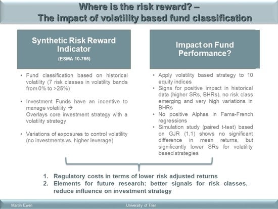
European regulation implicitly overlays the core strategy of a mutual fund under the UCITS (Undertakings for Collective Investment in Transferable Securities) regime with a long-term target volatility strategy, if investors are unwilling to accept a change in the risk class of their fund. Besides the implications for the risk profile of the fund stemming from the revised asset allocation and the potential systemic impact, this raises the question of how far it affects the returns that are delivered to investors. As the name Synthetic Risk Reward Indicator (SRRI) suggests, regulators have been aware that both dimensions have to be taken into account when assessing investment results.

Ewen and Rieger (2018) show that huge variations in exposures are required to maintain the risk classes prescribed. Notably very high levels of leverage are needed for higher risk classes to add variation in times of low volatilities. On the other hand, exposures are reduced massively in times of high volatilities. This mechanism may provide protection in downside markets. In this paper, we examine whether this interference in the investment process actually pays off for investors. The literature on volatility timing does not provide a clear-cut picture with respect to the effects on returns and, furthermore, focusses mostly on short-term volatilities in the analysis carried out. This paper extends research on volatility strategies by examining the impact on portfolio returns induced by a strategy that is using a long-term volatility as is introduced through the SRRI. As such a strategy is implicitly imposed by European regulators, the study also assesses the effects regulation have on investment results for investors. The findings of this paper may furthermore provide indications of how far the attribution of portfolio performance is diluted by the imposed trading signal.

The rest of the paper is organized as follows. Section 2 provides an overview of the regulatory background followed by a critical review of how it impacts fund management before concluding with a review of the literature on volatility timing. Section 3 describes in detail the investment strategy that is used to examine the impact of the SRRI. The subsequent Section 4 is dedicated to the application of this strategy to historical index data for ten worldwide equity indices. In Section 5, we conduct a simulation study to examine the differences on return distributions in a paired t-test. Section 6 concludes this paper.

2. Risk-Based Fund Classification

2.1. Regulatory Background

Since 1 July 2012, European investment funds that are incepted according to the UCITS regulation are obliged to publish a standard two-page document called the Key Investor Information Document (KIID), which aims to display general information and key figures of the fund to create more transparency and to enable investors to better compare investment alternatives. One key number to be displayed on this document is the SRRI (ESMA (2010)), which categorizes mutual funds with respect to their risk and return characteristics. As we will see below, the element “reward” in the nomenclature is somewhat misleading as the categorization is actually only carried out using risk characteristics. Generally, the SRRI aims to be a stable and comparable indicator of the riskiness of an investment alternative. It is based on the volatility of the weekly returns time series of the fund of the last five years as funds are classified according to the schedule shown in

Table 1. SRRI risk classes on corresponding volatility buckets as defined in the ESMA 10-673 guidelines.

SRRI Risk Classes
Risk Class	Volatility $\ge$	Volatility <
1	0%	0.5%
2	0.5%	2%
3	2%	5%
4	5%	10%
5	10%	15%
6	15%	25%
7	25%

.

The first step is to classify the mutual fund (or rather the targeted portfolio strategy) in one of five fund types (market, absolute return, total return, life cycle or structured fund). Without providing a clear-cut framework, European regulators (seem to) consider the following key determinants for the fund categorization:

• Investment across asset classes (if not and none of the others → market fund)
• Predefined risk limit (absolute return vs. total return)
• Change of the asset allocation over time (life cycle fund)
• Use of structured products (algorithm-based payoffs, date-specific payoffs, etc., → structured fund)

Depending on the fund type and data availability, the historical volatility of the time series of the fund’s returns or those of a representative asset mix (resp. benchmark) are considered to determine the SRRI. Further, in some cases, the volatility reverse engineered from the VaR limit or from a VaR number obtained in a simulation study is used to determine the SRRI. In the case of an absolute return or total return fund, the maximum of two or all three measures is taken, respectively. As mentioned earlier, the distinction between fund types is not determined clearly in the regulation. In any case, volatility plays an important role and will for most plain vanilla strategies for retail investors be the decisive metric for the SRRI.

If the current volatility of the fund falls outside the current bucket for more than 16 consecutive weeks, the SRRI (and consequently the KIID) has to be revised accordingly, and the portfolio migrates to the new risk class. Besides the administrative burden, this has further implications for the fund managers as the SRRI is intended to mirror the riskiness of the fund and to give investors a signal if the risk profile changes. The intended logic is as follows: if a fund, e.g., in Risk Class 4 migrates over time into Risk Class 6, this might not go along with a change in the risk appetite of its investors. Therefore, risk-averse investors could feel inclined to redeem their shares to invest in a less risky fund. Consequently, fund managers will have an incentive to manage the volatility of their portfolio in a way so as to keep it in a risk class that has been promised to investors.

2.2. Critical Review of the SRRI

2.2.1. Implications for Fund Returns

The implications of the SRRI will depend on the fund type chosen. However, for market funds and in certain cases for absolute/total return funds, the realized volatility is the decisive metric for the SRRI and as such needs to be monitored and controlled. Therefore, it is worth having a closer look at this metric with respect to its implications.

In the case of market funds, the concept of the SRRI effectively overlays the core investment strategy with a secondary investment principle based on the long-term ex-post volatility of the fund. This overlaying strategy will only be applied if investors are unwilling to accept the new risk class and exercise their power accordingly.

To avoid changes in the risk class, the portfolio manager either needs to reduce the risk in the portfolio, if the portfolio migrates to a riskier class, or increase the risk in the case of a transition to a less risky class. In the first case, the fund manager needs to deliver the realized mean of weekly returns in the upcoming weeks to add as little dispersion as possible and bring portfolio volatility back to the level he intends. In the second case, he needs to add as much variation (ideally to the positive side) as possible by raising the exposure, e.g., through derivatives. This will of course incur trading costs for investors, which will inevitably drag performance down.

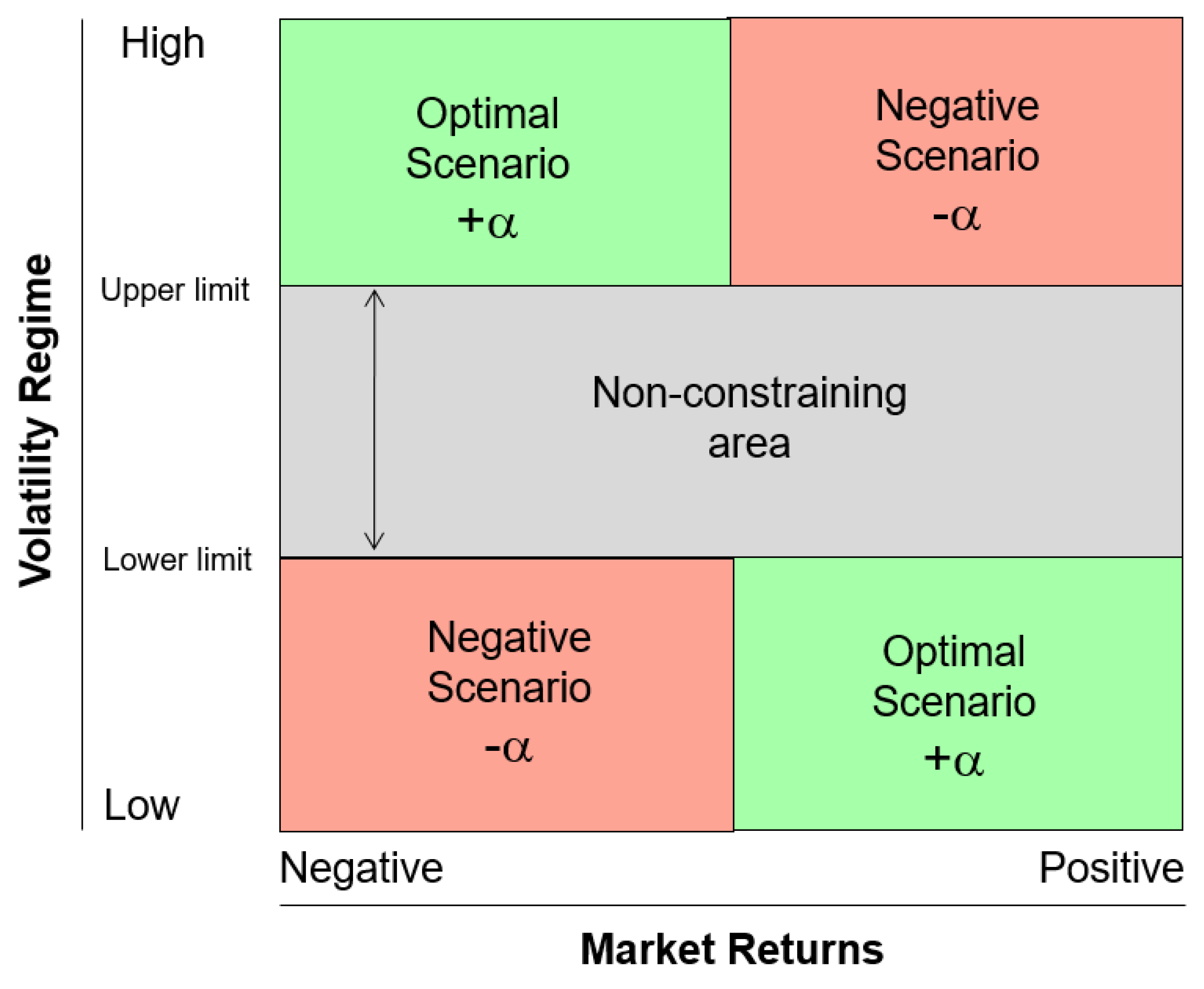
The revised investments will not only have an effect on the risk, but also on the return structure of the portfolio. Tail risk measures, such as the VaR, will indirectly be controlled by these volatility strategies, as well, due to the symmetrical nature of equity returns. This will of course only be the case if only linear assets are used to obtain market exposure.1

However, regarding the performance of such strategy, the situation is less clear cut. The potential scenarios for the overall impact on fund performance can be summarized in Figure 1. The table describes the different scenarios that arise if a binding restriction is created by the SRRI, that is to say if the current realized volatility falls outside the current band and the fund manager wants to avoid a migration to an adjacent risk class. If the periods with lower risk levels outside the current SRRI coincide with mostly positive returns, the over-investments will pay off, and vice versa for the case where the current volatility is higher. In this case, the portfolio can profit through avoided losses due to the under-investments triggered by the trading strategy, if these go along with higher negative returns. These situations are marked by the green boxes in the figure, whereas the red areas show the negative scenarios where the opposite is true, i.e., higher exposures to avoid a migration to lower risk classes in times of downside markets or reduced exposures to avoid higher risk classes in times of positive market trends.

2.2.2. Review of the Literature

Research on the intertemporal relation between risk and return does not provide a clear-cut picture. An extensive overview is for example provided in Bali (2008). Bali et al. (2009) found, using daily returns and time horizons from 1–6 months, that realized volatility has no predictive power for future returns. Ang et al. (2009) found that stocks with high idiosyncratic risk have low future returns. Harrison and Zhang (1999) found a positive relation between risk and return on horizons of one and two years. Further evidence for a positive relation was provided by Ghysels et al. (2005), Guo and Whitelaw (2006) and Bali (2008). Flemming et al. (2002) found that strategies based on volatilities outperform unconditionally-efficient strategies. Goyal and Santa-Clara (2003) also found a significant positive relation between risk and return, when both the systematic and idiosyncratic components are included. Adrian (2008) showed that long-term volatility has a positive relation to returns, whereas the short-term component is negatively related to the expected return. They suggest that this as a potential reason for the mixed results. Bali et al. (2009) presented evidence for a positive relation between return and downside risk.

Without providing conclusive evidence, some studies suggested that volatility may be used as a trading signal to generate overall positive returns. However, none of the studies used a long-term horizon, i.e., five-year volatility, as prescribed by the SRRI.

3. Investment Strategy Based on the SRRI

As mentioned above, if the SRRI creates a binding mechanism for fund managers, it basically introduces a long-term volatility trading strategy that overlays the core strategy of the portfolio. That is to say, it creates a trading signal to either reduce the amount of risk in the portfolio in times of high volatility (compared to the current volatility band) or to add more risk to the portfolio in times of lower volatility. To capture the impact of such trading strategy on the characteristics of fund performance, we carry out a historical backtesting and a simulation study that uses the SRRI as a trading signal.

Ewen and Rieger (2018) have shown that some portfolios that fall under the SRRI have limited possibilities to raise exposures in times of lower volatilities. These portfolios may not be able to maintain the risk classes. However, the analyses conducted revealed that those portfolios with unlimited leverage possibilities work quite well, maintaining the risk classes within the limits of practical constraints when high contributing observations shoot the strategies up in a higher risk band.

We therefore consider a trading rule that follows an equity index and only alters the exposure according to the following rule:

This leads to the following trading strategy:

$$E(\sigma ,n)=\left\{\begin{array}{cc}0,& \mathrm{if} {\sigma }_{t-1}>ub\hfill \\ 2^{\lfloor \frac{n}{4}+1\rfloor },& \mathrm{if} {\sigma }_{t-1,\dots ,t-s}<lb,n\in {\mathbb{N}}^{+}\hfill \\ 1,& \mathrm{else}\hfill \end{array}\right.$$

where:

• E = the exposure to the index
• $\sigma$ = the annual volatility of weekly returns calculated for the purposes of the synthetic risk reward indicator (ESMA 10-673)
• n = the number of weeks where $\sigma$ has been consecutively below lb, and $\lfloor x\rfloor$ denotes the integer part of x
• $ub$ = upper bound of the selected risk class
• $lb$ = lower bound of the selected risk class

Therefore, basically, the portfolio follows a risk on-risk off strategy if the SRRI of the previous period falls outside the current band. If the upper bound is breached, the exposure is reduced to zero, whereas the exposure is doubled for the next period if the previous SRRI falls below the the lower bound.2 The exposure is doubled again in case the lower bound is not reached within four weeks. This pattern is repeated until the volatility is high enough to fall in the desired risk class again. If it lies within the current band, the fund is just invested 100% in the index. When the portfolio is not invested in the index, we assume an investment in the risk-free rate.

Using passive indices has the advantage of isolating the effect of the SRRI implied trading rule on fund performance from any trading activity performed by fund managers. As in the previous section, our focus is on equity markets, so we focus on Risk Classes 5–7. Lower risk classes would obviously match with the risk levels associated with balanced or fixed income funds, requiring a different asset. Furthermore, these ranges for these risk classes have been closest historically to those of most equity indices. Furthermore, Ewen and Rieger (2018) showed that lower risk classes do not seem adequate for equity funds, as they would not allow for fund management within the realms of practicability. Our analyses is carried out on standard equity indices, where in practice, the variations in exposures could be easily obtained through futures contracts on the indices.

4. Backtesting on Historical Data for Equity Indices

We conduct our analysis on a set of worldwide equity indices. We use price indices that were obtained from the Thomson Reuters database. The risk-free rates were obtained from Kenneth French’s web page. We have access to weekly return data for the period 13 September 1991–27 February 2015. For comparison purposes, we also apply a traditional trading strategy, which permanently invests according to a 70/30 rule, 70% in the index and 30% in risk-free assets. We examine Risk Classes 5–7, which means that the strategies in our analysis have a minimum volatility of 10% per annum. The descriptive statistics of our sample are shown in

Table 2. This table shows the descriptive statistics of the equity indices used in our analysis. Volatility is calculated as per the ESMA 10-788 guidelines. The setup for the Value at Risk (VaR) is CI 0.99, 5 days (weekly returns). SR, Sharpe Ratio.

Metric/Index	S&P 500	Euro Stoxx 50	DAX	FTSE	CAC 40	IBEX 35	Hang Seng	Dow Jones	MSCI World	NASDAQ
Volatility	0.1671	0.1870	0.2219	0.1684	0.2116	0.2207	0.2461	0.1623	0.1602	0.2548
Mean	0.0016	0.0013	0.0021	0.0011	0.0012	0.0016	0.0021	0.0017	0.0013	0.0029
Min	−0.1820	−0.2318	−0.2161	−0.2105	−0.2216	−0.2120	−0.1806	−0.1815	−0.2007	−0.2530
Max	0.1203	0.1455	0.1612	0.1341	0.1324	0.1455	0.1493	0.1129	0.1237	0.2109
VaR	0.0603	0.0669	0.0742	0.0632	0.0751	0.0732	0.0979	0.0577	0.0553	0.0926
SR	0.0712	0.0505	0.0669	0.0453	0.0421	0.0526	0.0610	0.0765	0.0569	0.0817

.

4.1. Historical Performance Parameters of Volatility-Based Strategies

The results are given in

Table 3. Results of the SRRI-based trading strategy. If the realized volatility of the strategy falls outside the range defined by the risk class, the exposure is altered by a trading rule based on volatility buckets. The table shows the mean values for the respective metric of the strategies applied to weekly returns for the period from 13 September 1991–27 February 2015. For reference purposes, we also added the results for the index itself, representing a passive investment and a traditional 70/30 strategy (TR). The highest mean returns are obtained for Risk Class 7 (RC7), whereas a diverse pictures is shown regarding the SRs (Sharpe Ratios) with no risk class clearly emerging.

Metric	Strategy	S&P 500	SX5E	DAX	FTSE	CAC 40	IBEX 35	Hang Seng	DJ Ind	MSCI World	NASDAQ
Max	Index	0.1203	0.1455	0.1612	0.1341	0.1324	0.1455	0.1493	0.1129	0.1237	0.2109
	TR	0.0842	0.1021	0.1129	0.0939	0.0927	0.1021	0.1048	0.0791	0.0866	0.1480
	RC7	0.6157	0.3246	0.4585	0.4237	0.4270	0.4347	0.3093	0.6432	0.5780	0.4569
	RC6	0.3075	0.1689	0.1612	0.1341	0.1324	0.1455	0.1493	0.2629	0.2215	0.1243
	RC5	0.0758	0.1194	0.1612	0.0827	0.0888	0.0836	0.1687	0.0843	0.0814	0.0923
Mean	Index	0.0016	0.0013	0.0021	0.0011	0.0012	0.0016	0.0021	0.0017	0.0013	0.0029
	TR	0.0013	0.0011	0.0016	0.0009	0.0010	0.0013	0.0016	0.0014	0.0011	0.0022
	RC7	0.0029	0.0011	0.0027	0.0013	0.0022	0.0025	0.0029	0.0034	0.0022	0.0037
	RC6	0.0020	0.0014	0.0016	0.0011	0.0009	0.0015	0.0024	0.0022	0.0017	0.0035
	RC5	0.0013	0.0006	0.0022	0.0005	0.0003	0.0009	0.0020	0.0014	0.0010	0.0022
Min	Index	−0.1820	−0.2319	−0.2161	−0.2105	−0.2216	−0.2120	−0.1806	−0.1815	−0.2007	−0.2530
	TR	−0.1273	−0.1622	−0.1512	−0.1473	−0.1551	−0.1483	−0.1261	−0.1270	−0.1404	−0.1768
	RC7	−0.3682	−0.4127	−0.4263	−0.4418	−0.8164	−0.3350	−0.2365	−0.3429	−0.3901	−0.3244
	RC6	−0.1820	−0.2319	−0.2161	−0.2105	−0.2216	−0.2120	−0.1806	−0.1815	−0.2007	−0.1746
	RC5	−0.1820	−0.2319	−0.1289	−0.2105	−0.3089	−0.2120	−0.1200	−0.1815	−0.2007	−0.2530
SR	Index	0.0712	0.0505	0.0669	0.0453	0.0421	0.0526	0.0610	0.0765	0.0569	0.0817
	TR	0.0817	0.0599	0.0748	0.0557	0.0504	0.0605	0.0681	0.0873	0.0679	0.0886
	RC7	0.0746	0.0297	0.0701	0.0338	0.0505	0.0666	0.0733	0.0864	0.0557	0.0876
	RC6	0.0791	0.0505	0.0582	0.0448	0.0310	0.0511	0.0796	0.0882	0.0720	0.1208
	RC5	0.0727	0.0279	0.1059	0.0244	0.0122	0.0403	0.0876	0.0796	0.0536	0.1078
VaR	Index	0.0603	0.0669	0.0742	0.0632	0.0751	0.0732	0.0979	0.0577	0.0553	0.0926
	TR	0.0422	0.0469	0.0520	0.0443	0.0525	0.0514	0.0685	0.0406	0.0388	0.0649
	RC7	0.0905	0.0910	0.0936	0.0971	0.0990	0.0953	0.1065	0.1114	0.0872	0.1121
	RC6	0.0703	0.0777	0.0721	0.0721	0.0724	0.0696	0.0948	0.0690	0.0663	0.0744
	RC5	0.0464	0.0484	0.0543	0.0447	0.0538	0.0517	0.0762	0.0467	0.0408	0.0576
Vol	Index	0.1671	0.1870	0.2219	0.1685	0.2116	0.2207	0.2461	0.1623	0.1602	0.2548
	TR	0.1170	0.1309	0.1553	0.1179	0.1481	0.1545	0.1723	0.1136	0.1121	0.1784
	RC7	0.2808	0.2698	0.2769	0.2666	0.3121	0.2753	0.2805	0.2806	0.2791	0.3061
	RC6	0.1862	0.1972	0.2044	0.1801	0.2041	0.2071	0.2192	0.1809	0.1753	0.2063
	RC5	0.1295	0.1446	0.1485	0.1384	0.1586	0.1539	0.1650	0.1302	0.1290	0.1497

. The realized volatilities of the strategies show the expected pattern as they decline with the lower risk classes and raise with higher risk classes. Apart from some exceptions for Risk Class 5, all average volatilities lie in the targeted ranges. Higher volatilities outside the prescribed band are observed for Risk Class 5 for the IBEX 35 and Hang Seng. These are arguably high risk indices, so these results may not be surprising for Risk Class 5. Given the average volatilities for these two indices of 22.07% and 24.61%, respectively, Risk Class 5 may not be an adequate choice here.

The average volatilities of Risk Class 7 and also half of the indices in Risk Class 6 are higher than those of the respective index. The traditional strategy is aligned with Risk Class 5 when looking at the realized volatility. Looking at the VaR, one finds that the VaR develops along with the risk classes in a similar way as volatility, that is to say it declines with lower risk classes and raises with higher risk classes. Therefore, controlling the volatility of portfolio investing in linear assets effectively also controls the tail risk of the portfolio in a similar way. This result is expected given the mostly symmetrical distribution of equity returns.

Looking at the return side, the portfolios in Risk Class 7 show the highest mean returns, whereas on a (dispersion) risk adjusted basis, the picture is more diverse. For seven out of our 10 indices, the volatility-based strategies show the highest SRs without one of them clearly emerging. In three cases, the traditional strategy yields the best results. Generally, we can state that the volatility-based strategies yield better SRs than passive investments in the index for our observation window.

4.2. Buy and Hold Returns

In order to gain a more dynamic perspective, we examine the Buy and Hold Returns (BHR) of the strategies. They are are calculated over the whole sample period through the following formula:

$$BH{R}_{i,t}=\prod _{t=1}^n(1+r_{i,t})$$

(1)

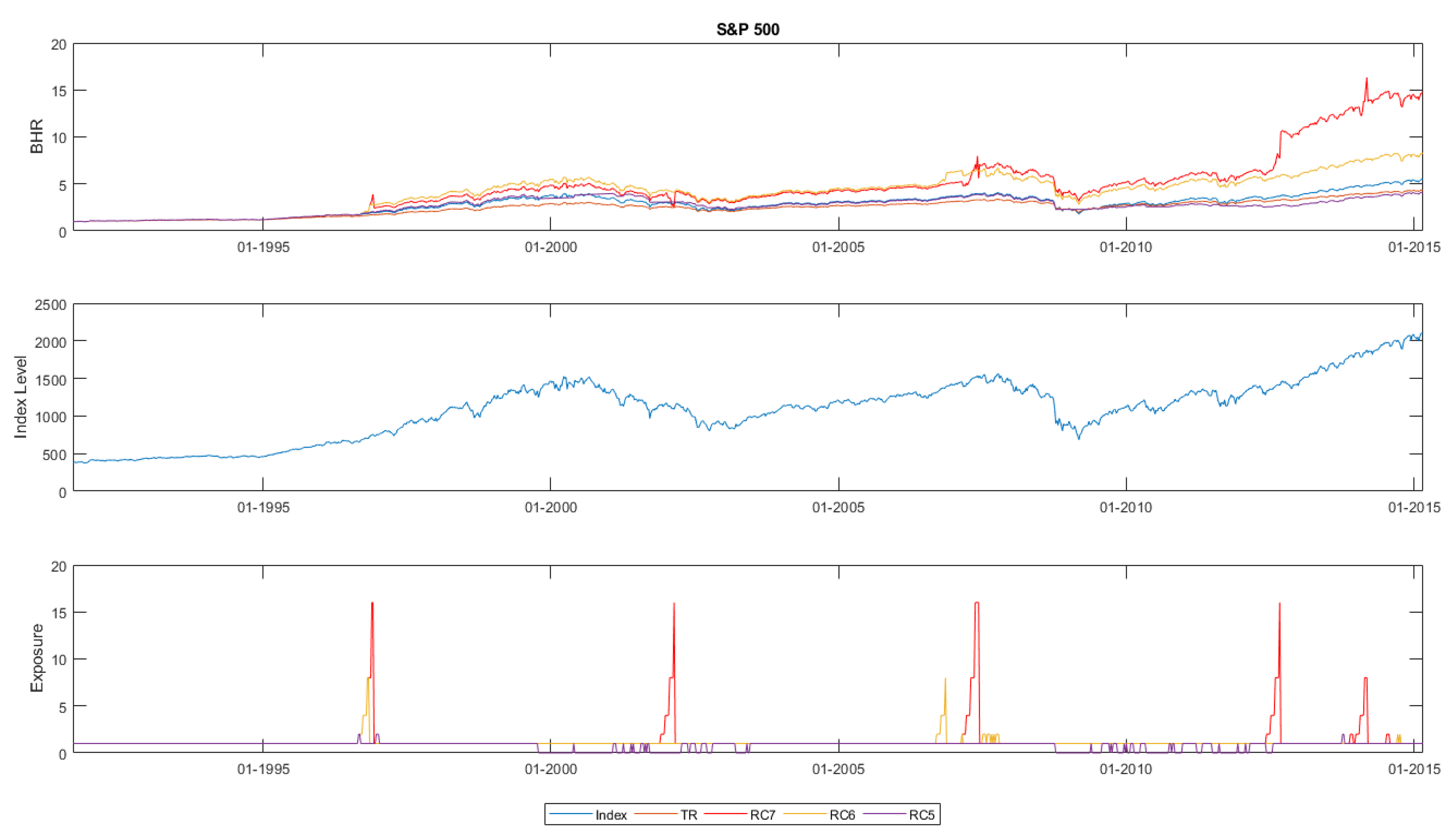
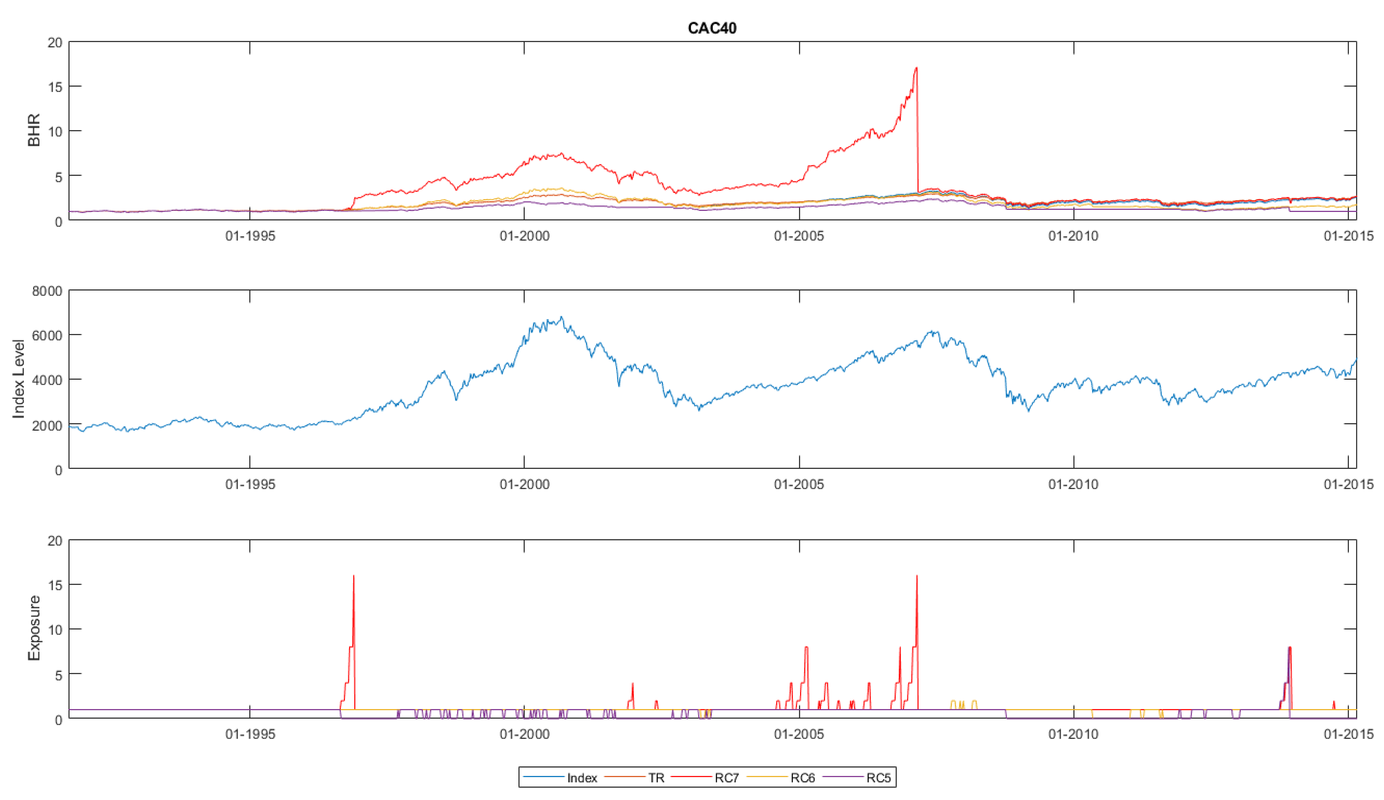
We find that for all of the indices, one of the volatility-based trading strategies displays higher BHRs than the passive index or the traditional strategies. For most of the indices, Risk Classes 6 or 7 yield the highest BHRs for our observation window. We can, however, also state that these go along with notably higher variations for these risk classes compared to a passive investment. The outperformance of the strategies comes in most of the cases from higher participations during the upside markets, e.g., during the 1990s or more recently in the years after the Lehman event (see, e.g., S&P or CAC 40 in Figure 2 and Figure 3).

It should be noted that Risk Classes 6 and 7 (the latter even more so) provide a very low level of protection in downside markets, which leads to more variations in the BHRs than, e.g., the passive investments. A very striking example of this is shown in Figure 3. We refer to Risk Class 7 for the CAC 40, which is invested with a leverage of 1600% during a steep downside market in 2007 and consequently suffers a massive reduction in BHRs. Such protection would on the other hand be expected with Risk Class 5. However, we observe that this mechanism only kicks in delayed also for Risk Class 5 in most of the cases. This pattern is particularly pronounced when disruptive events like the Lehman crisis happens.

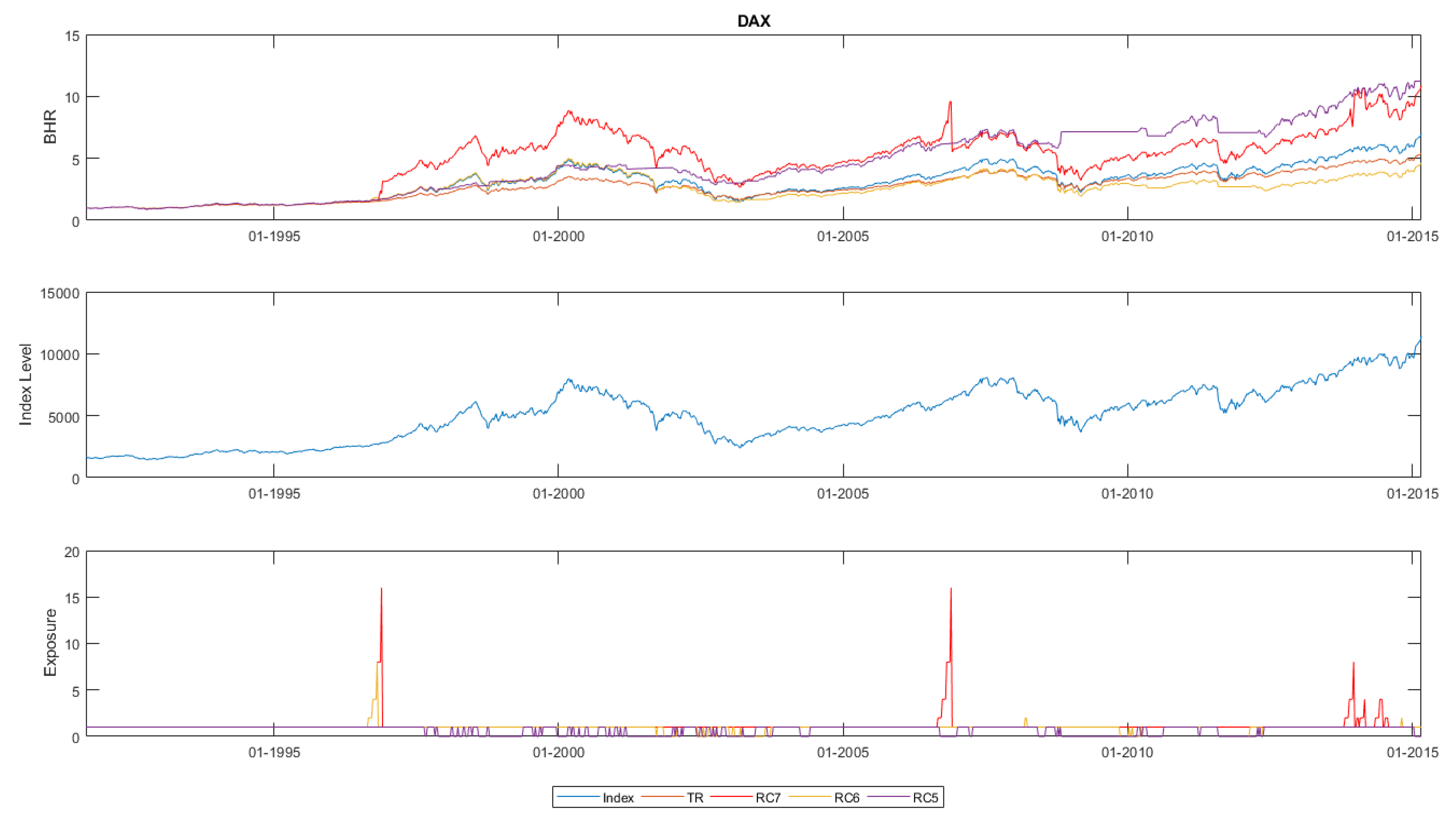
On the other side, the signal to re-invest again is given too late in some cases when markets rebound, so in particular, Risk Class 5 misses out on participating in upside markets in the second half of the 1990s or most recently after the Lehman event (e.g., refer to Figure 2 or Figure 3). In fact, full protection for downside markets in Risk Class 5 only proves to be valid for the DAX, where losses are avoided during both the technology and the Lehman event (Figure 4). Consequently Risk Class 5 yields the best BHRs in this index before transaction costs.

So far, we can state that from a return perspective our historical backtesting, the volatility-based strategies provide some evidence for better performance of these against indices. Regarding the BHRs, the higher levels of returns are also associated with higher variations in BHRs. We find indications that the signal prescribed by the SRRI tends to be late in dynamic market environments.3

4.3. Risk Adjusted Returns

Without providing a clear-cut picture, our analyses so far point to the better performance of the volatility-based strategies. Next, we run Fama and French (1992) three-factor regressions on the strategies to examine whether there is an economic value of the volatility strategy in equity markets accounting for the size and value effect. The factor data were obtained from Kenneth French’s website

$$E\left(r_i\right)={\beta }_0+{\beta }_1\ast E(r_m-r_f)+{\beta }_2\ast SMB+{\beta }_3\ast HML+{ϵ}_i$$

(2)

where:

• $E\left(r_i\right)$ = the expected return of asset i
• $rf$ = the risk-free rate
• $E\left(r_m\right)$ = the expected return of the market portfolio
• $SMB$ = the returns of the size factor
• $HML$ = the returns of the value factor
• ${ϵ}_i$ = the IID error term

The results are presented in

Table 4. This table shows the first set of results of the Fama–French three-factor regressions that were performed to verify if the volatility-based strategies yielded significant outperformance. Significance at a confidence level of 99%, 95%, 90% is indicated with ***, **, *, respectively. No significant alphas at the 99%-level could be found for the investment strategies based on the risk classes.

		S&P 500		SX5E		DAX		FTSE		CAC 40
		Beta	t-stat	Beta	t-stat	Beta	t-stat	Beta	t-stat	Beta	t-stat
RC7	Constant	0.0685	0.84	−0.0978	−1.14	0.0464	0.54	−0.0777	−0.89	−0.0138	−0.14
	Market	1.1343 ***	32.51	0.9613 ***	26.22	1.0226 ***	27.93	0.8963 ***	24.00	1.0552 ***	24.25
	SMB	−0.3428 ***	−5.28	−0.1035	−1.52	0.0476	0.70	−0.1317 *	−1.90	0.0009	0.01
	HML	0.0363	0.58	0.1218 *	1.87	0.1153 *	1.77	0.1924 ***	2.89	0.2126 ***	2.75
RC6	Constant	−0.0032	−0.12	−0.0497	−0.90	−0.0249	−0.41	−0.0752	−1.52	−0.1068	−1.84
	Market	1.0233 ***	87.60	0.8353 ***	35.60	0.8116 ***	31.64	0.7750 ***	36.83	0.8472 ***	34.19
	SMB	−0.2279 ***	−10.48	−0.1461 ***	−3.35	0.0217	0.46	−0.0592	−1.51	−0.0866 *	−1.88
	HML	0.0130	0.62	0.1144 ***	2.74	0.1188 ***	2.60	0.2034	5.43	0.1618 ***	3.67
RC5	Constant	−0.0001	0.00	−0.0602	−1.20	0.1048 **	1.99	−0.0681	−1.45	−0.0876	−1.53
	Market	0.5737 ***	40.30	0.4229 ***	19.83	0.3912 ***	17.43	0.4256 ***	21.27	0.3948 ***	16.18
	SMB	−0.2084 ***	−7.87	−0.1181 ***	−2.98	0.0113	0.27	−0.1478 ***	−3.97	−0.0211	−0.47
	HML	−0.1120 ***	−4.42	−0.0277	−0.73	−0.0591	−1.48	−0.0375	−1.05	−0.0319	−0.73

and

Table 5. This table shows the second set of results of the Fama–French three-factor regressions that were performed to verify if the volatility-based strategies yielded significant outperformance. Significance at a confidence level of 99%, 95%, 90% is indicated with ***, **, *, respectively. Apart from the NASDAQ, no significant alphas at the 99%-level could be found.

		IBEX 35		Hang Seng		DJ Ind		MSCI World		NASDAQ
		Beta	t-stat	Beta	t-stat	Beta	t-stat	Beta	t-stat	Beta	t-stat
RC7	Constant	0.0356	0.40	0.1103	1.10	0.1203	1.40	−0.0009	−0.01	0.1712 ***	2.41
	Market	0.9319 ***	24.36	0.7233 ***	16.89	1.0593 ***	28.87	1.0258 ***	27.50	1.2930 ***	42.69
	SMB	0.0581	0.82	0.0596	0.75	−0.4195 ***	−6.14	−0.2088 ***	−3.01	0.1175 **	2.08
	HML	0.2581 ***	3.79	0.0798	1.05	0.1551 ***	2.37	0.1370 **	2.06	−0.8828 ***	−16.37
RC6	Constant	−0.0367	−0.56	0.0971	1.22	0.0216	0.64	−0.0278	−0.80	0.1600 ***	3.31
	Market	0.7509 ***	27.03	0.5266 ***	15.50	0.9444 ***	65.04	0.9010 ***	60.92	0.9265 ***	44.89
	SMB	0.0104	0.20	0.0729	1.15	−0.3121 ***	−11.55	−0.0582 **	−2.11	0.1575 ***	4.10
	HML	0.1699 ***	3.44	0.0772	1.28	0.1214 ***	4.70	0.1450 ***	5.51	−0.2776 ***	−7.56
RC5	Constant	−0.0266	−0.48	0.1123 *	1.76	0.0139	0.40	−0.0279	−0.79	0.1054 **	2.14
	Market	0.3738 ***	15.71	0.2058 ***	7.57	0.5575 ***	37.25	0.5359 ***	35.49	0.4246 ***	20.17
	SMB	−0.0217	−0.49	0.1371 ***	2.71	−0.2898 ***	−10.41	−0.1524 ***	−5.42	0.2569 ***	6.56
	HML	−0.0122	−0.29	−0.0689	−1.42	−0.0503 *	−1.89	−0.1572 ***	−5.85	−0.1775 ***	−4.74

. As is visible from the tables, with one exception, none of the volatility-based strategies applied to the indices yielded alphas in either direction at relevant significance levels. Significant positive alphas at the 99%-level can be observed for the NASDAQ, here for all risk classes. Risk Class 5 for the DAX shows a positive alpha at the 95%-level, which supports the positive results for this risk class and the DAX from the analysis of the BHRs. Apart from these two exceptions, no significant alphas could be found, so overall, only a very limited positive impact of the SRRI could be found accounting for the size and value effect. On the other hand, we also did not find any indication for indirect costs induced by the volatility bands. Given the results above, we abstain from adding further factors capturing momentum (Carhart (1997)) or liquidity (Pastor and Stambaugh (2003)) to the analysis.

4.4. Discussion

Overall, we can state that the historical backtesting of a risk on-risk off trading strategy based on the SRRI proves to effectively control dispersion and tail risk on a long-term basis. Furthermore, we find evidence in our analysis on historical data for equity indices that the volatility strategy imposed by regulators would actually be beneficial for equity investors in terms of higher SRs and BHRs compared to a passive investment in the index. It should however be noted that none of strategies clearly emerges either regarding BHRs, nor the SRs. Further to this, very high variations of the BHRs are observable. We can also observe that high leverage induced by low volatility levels or lagged reaction to cut exposures in downside markets may be detrimental to performance.

This is a pitfall of the long-term orientation of the setup, which aims to generate stable risk classes. We should also mention at this stage that we abstract from trading costs in our analyses; this will of course further reduce the the performance of the volatility strategies, even if the exposure can be achieved in a cost-efficient way through futures contracts. Accounting for the size and value effect reveals no significant alphas in most of the cases. In the following, we conduct a simulation study to gain further evidence of the impact of the volatility strategy on the distribution parameters of returns. We should also point out at this stage that we abstract from trading costs in our analysis; these will of course reduce any positive impact induced by the SRRI.

5. Simulation Study

5.1. Design of the Simulation

The analysis so far has been carried out only on historical data and has not provided a clear picture. In order to examine the effect of the SRRI on the distribution parameters of portfolio returns in statistical tests, we conduct a simulation study. We estimate a GARCH model on the return time series of each index. These models are then used to generate 10,000 price paths of 1040 weekly returns (i.e., 20 years). The volatility strategy from Section 3 is then applied to these generated returns. We then use the obtained returns from the strategies to compute the distribution parameters and risk metrics for each price path. A paired t-test is subsequently performed on these parameters between the simulated passive returns and the returns of the strategies, maintaining the risk classes as defined above. To limit the impact of extreme scenarios, we constrain our investment strategy to a maximum leverage of 3200%. This level of leverage would only be surpassed after six months outside the selected risk band.

We generate the returns using two specifications. First, we use a GARCH(1,1)-model as, e.g., described in Engle (2001) or Engle and Patton (2001).

$${\sigma }_n^2=\gamma V_L+\alpha u_{n-1}^2+\beta {\sigma }_{n-1}^2$$

(3)

where:

• ${\sigma }_n^2$ = the conditional variance of returns in n
• $V_L$ = the unconditional variance of returns
• $u_{n-1}^2$ = the squared residuals for period $n-1$

Setting $\omega =\gamma V_L$, the GARCH(1,1) Equation (3) can be written as:

$${\sigma }_n^2=\omega +\alpha u_{n-1}^2+\beta {\sigma }_{n-1}^2$$

(4)

In the second setup, we estimate a GJR-GARCH(1,1)-model as, e.g., described in Glosten et al. (1993), which is then used to simulate the returns. This specification accounts for asymmetry (or leverage) within the volatility modelling and takes the following form:

$${\sigma }_n^2=\gamma V_L+\alpha u_{n-1}^2+\beta {\sigma }_{n-1}^2+{\gamma }_{+}I(u_{n-1}^2>0)+{\gamma }_{-}I(u_{n-1}^2<0)$$

(5)

The model parameters are estimated on the return data described above using the full time series available. Within the simulation, we assume a t-distribution for the innovations.

5.2. Results

As you can see from

Table 6. Results of the paired t-test on the distribution parameters. Significance at a confidence level of 99%, 95%, 90% is in indicated with ***, **, *, respectively. The returns are generated with a GJR(1,1)-model, where the parameters for each index are estimated on the full history available and a t-distribution is assumed for the innovations. We generate 10,000 price paths of 1040 weekly returns and apply the risk on-risk off strategy. Then, the distribution parameters and the Sharpe ratios are calculated, and the t-test is performed against the same parameters of the passive strategy. There is no significant difference in mean return, but the strategies based on volatility display significantly lower SRs.

	Strategy	S&P 500	SX5E	DAX	FTSE	CAC 40	IBEX 35	Hang Seng	DJ Ind	MSCI World	NASDAQ
RC7	Mean	−0.45	−0.15	0.67	1.00	0.47	0.52	1.27	−0.44	−2.14 **	1.06
	Volatility	223.61 ***	218.41 ***	151.93 ***	289.54 ***	181.54 ***	149.18 ***	71.90 ***	309.71 ***	495.76 ***	73.55 ***
	Skewness	−2.58 ***	−2.99 ***	−1.23	−1.90 *	−0.60	−0.60	−0.15	−2.00 **	−2.28 **	−0.41
	Kurtosis	49.40 ***	47.85 ***	35.92 ***	54.08 ***	43.09 ***	39.23 ***	22.91 ***	54.19 ***	61.87 ***	23.35 ***
	VaR	−152.95 ***	−151.11 ***	−111.59 ***	−177.70 ***	−126.74 ***	−109.31 ***	−57.70 ***	186.22 ***	−227.48 ***	−58.57 ***
	SR	−16.31 ***	−13.79 ***	−10.00 ***	−12.23 ***	−11.24 ***	−10.89 ***	−6.57 ***	−13.09 ***	−11.17 ***	−7.08 ***
RC6	Mean	0.77	0.53	−0.46	0.31	0.10	0.11	0.25	0.16	−0.30	0.60
	Volatility	−19.62 ***	−25.18 ***	−43.51 ***	−8.17 ***	−39.10 ***	−50.61 ***	−79.73 ***	−5.02 ***	68.79 ***	−78.83 ***
	Skewness	−7.80 ***	−8.98 ***	−11.37 ***	−4.38 ***	−11.84 ***	−11.13 ***	−7.81 ***	−4.67 ***	−1.73 *	−5.30 ***
	Kurtosis	16.82 ***	12.34 ***	3.50 ***	15.81 ***	10.02 ***	11.43 ***	38.42 ***	15.27 ***	26.10 ***	25.56 ***
	VaR	16.21 ***	18.79 ***	29.29 ***	8.20 ***	25.52 ***	32.54 ***	53.06 ***	6.07 ***	−42.59 ***	52.31 ***
	SR	−15.12 ***	−12.19 ***	−11.62 ***	−12.02 ***	−10.76 ***	−11.22 ***	−10.68 ***	−11.50 ***	−10.66 ***	−10.56 ***
RC5	Mean	−0.87	−0.84	−1.15	−0.22	−0.68	−0.80	−0.47	−0.47	−1.10	−0.44
	Volatility	−91.68 ***	−134.49 ***	−241.36 ***	−111.24 ***	−233.53 ***	−251.96 ***	−176.97 ***	−103.69 ***	−78.84 ***	−177.97 ***
	Skewness	−8.04 ***	−4.77 ***	−0.30	−11.58 ***	−3.84 ***	−1.66	5.26 ***	−7.93 ***	−12.31 ***	4.41 ***
	Kurtosis	21.85 ***	26.29 ***	46.92 ***	24.02 ***	66.47 ***	79.86 ***	99.96 ***	12.55 ***	10.91 ***	82.13
	VaR	56.56 ***	73.28 ***	111.20 ***	64.02 ***	104.82 ***	109.13 ***	89.16 ***	60.56 ***	46.49 ***	89.21
	SR	−15.62 ***	−11.95 ***	−7.13 ***	−12.97 ***	−7.79 ***	−7.37 ***	−4.83 ***	−12.89 ***	−12.32 ***	−4.89 ***

, we find that applying the strategies has a significant impact on the volatilities of the portfolios. That is to say, for the strategy in Risk Class 7, the volatility is significantly higher at the 99%-level than the index volatility and vice versa for Risk Classes 5 and 6.4 The same picture with switched signs emerges for the tail risk measure (VaR), so overall, the findings indicate that the volatility-based strategies without leverage constraints have a significant effect on volatility and VaR. This is a pattern one would expect given the results from the analyses of historical data and once again underpins the effectiveness of the trading rule applied in controlling portfolio volatility.

Apart from Risk Class 7, where most of the indices do not show any significant difference in skewness, we observe significantly lower skewness for Risk Classes 5 and 6. The volatility-based strategies show higher levels of kurtosis than the index itself, which is a result of the risk on-risk off strategy, as they will cumulate many returns close to zero due to the periods of under-investments. The higher levels of kurtosis also show that the volatility strategy would broaden the occurrences of returns, i.e., more extreme or higher values and less occurrences around the mean induced by higher leverage. So far, the results are as expected considering the trading rule applied.

We could not find significant differences in the mean returns between the two samples, so the long-term volatility strategy imposed by the SRRI does not seem to affect average returns materially. Looking at the risk adjusted measure, we can observe negative t-statistics for the SRs for all the indices. This indicates a negative impact on performance considering both risk and return. We can therefore state that the indications for positive impact found in the historical analysis were not confirmed in our simulation study. To the contrary, our results suggest a negative impact on the results for investors. For robustness checks, we change the time window taken into account when estimating the model parameters for both models. The results remain unchanged.5

Overall, we can state that the SRRI yields significantly lower risk adjusted returns, while average returns do not seem to be affected in the same way. This suggests that higher variations induced by the volatility signal do not pay off on a risk adjusted basis. It should also be noted at this stage that our analysis is before trading costs, which will have a further negative impact on the final result for investors.

As we have shown above, this finding may be related to the fact that the long-term volatility is used as a signal (weekly data from the last five years). Consequently, the strategy will be notoriously late as it will only react if there is a clear trend or a very large move that leads to a rather quick adaptation of the estimate. Short-term volatilities might prove to be more efficient in creating a trading signal in the context of a volatility trading strategy, potentially at the cost of less stable risk classes, though.

6. Conclusions

We examine the impact of the long-term volatility strategy imposed by the SRRI on the returns of equity investment strategies. In our historical backtesting of the volatility strategies, we initially found indications that for some indices, they actually yielded higher SRs and also higher BHRs than passive investments in the index; the latter albeit at the cost of notably higher variations. Besides a few exceptions, the analyses of the BHRs revealed that realized volatility as the signal chosen for the risk classes did not provide robust protection in downside markets. It should also be noted that none of the risk classes clearly stood out as an optimal risk class.

For most of the worldwide indices, no significant alphas emerged for the SRRI-based strategies accounting for the size and value effect. In further analyses through a simulation study, we could not find evidence for a significant effect on mean returns in a paired t-test. The results did, however, reveal significantly lower Sharpe ratios earned by the volatility-based strategies. This suggests that investors may have to bear additional indirect costs through lower risk adjusted returns. Consequently, controlling a portfolio’s volatility according to the SRRI can lead to additional regulatory costs. Furthermore, distortions when attributing fund performance were evident.

Potential future research could focus on improvements regarding the return effects induced by the SRRI by, e.g., considering flexible boundaries or a more refined set of indicators for the determination of the risk class.