On a Multiplicative Multivariate Gamma Distribution with Applications in Insurance

Abstract

One way to formulate a multivariate probability distribution with dependent univariate margins distributed gamma is by using the closure under convolutions property. This direction yields an additive background risk model, and it has been very well-studied. An alternative way to accomplish the same task is via an application of the Bernstein–Widder theorem with respect to a shifted inverse Beta probability density function. This way, which leads to an arguably equally popular multiplicative background risk model (MBRM), has been by far less investigated. In this paper, we reintroduce the multiplicative multivariate gamma (MMG) distribution in the most general form, and we explore its various properties thoroughly. Specifically, we study the links to the MBRM, employ the machinery of divided differences to derive the distribution of the aggregate risk random variable explicitly, look into the corresponding copula function and the measures of nonlinear correlation associated with it, and, last but not least, determine the measures of maximal tail dependence. Our main message is that the MMG distribution is (1) very intuitive and easy to communicate, (2) remarkably tractable, and (3) possesses rich dependence and tail dependence characteristics. Hence, the MMG distribution should be given serious considerations when modelling dependent risks.

1. Introduction

Let $\mathcal{X}$ be a collection of actuarial risks, that is let it contain random variables (r.v.’s) $X:\Omega \to \mathbf{R}$ defined on the probability space $(\Omega ,\mathcal{F},\mathbf{P})$ and interpreted as the financial risks an insurer is exposed to. Often, for applications in insurance, actuaries would consider those $X\in \mathcal{X}$, whose distributions are supported on the non-negative real half-line, have positive skewness, and allow for a certain degree of heavy-tailness. One such distribution, which has been of prominent importance in insurance applications, is gamma. We refer to Hürlimann (2001), Dornheim and Brazauskas (2007), Furman et al. (2018), and Zhou et al. (2018) for applications in solvency assessment, loss reserving, and aggregate risk approximation, respectively.

Furthermore, let $\gamma \in {\mathbf{R}}_{+}$ and $\sigma \in {\mathbf{R}}_{+}$ denote, correspondingly, the shape and scale parameters, then the r.v. X is said to be distributed gamma, succinctly $X\sim Ga(\gamma ,\sigma )$, if it has the probability density function (p.d.f.)

$$f\left(x\right)=\frac{1}{\Gamma \left(\gamma \right)}{e}^{-x/\sigma }{x}^{\gamma -1}{\sigma }^{-\gamma }\mathrm{for}\mathrm{all}x\in {\mathbf{R}}_{+},$$

(1)

where $\Gamma (·)$ stands for the complete gamma function. The popularity of the r.v.’s distributed gamma in insurance applications is not surprising: the p.d.f.’s of the (aggregate) insurance losses have as a rule the same shape as p.d.f. (1), i.e., they are positively skewed, unimodal and have positive supports; p.d.f. (1) is log-convex for $\gamma \in (0,1)$ and so has decreasing failure rate, thus allowing for moderate heavy-tailness (Klugman et al. 2012); p.d.f. (1) has been very well studied and has turned out remarkably tractable.

When it comes to multivariate extensions of p.d.f. (1), there are an ample number of dependence structures with univariate margins distributed gamma to consider (e.g., Kotz et al. 2000; Balakrishnan and Ristić 2016, for a recent development and a comprehensive reference, respectively). However, irrespective of whether the two-steps copula approach or the more ‘natural’ stochastic representation approach to formulate the desired multivariate gamma distribution is pursued, the tractability of the end-result is often an issue. For the former approach, the cumulative distribution function (c.d.f.) of (1) cannot be written in a closed form, and consequently intensive numerical algorithms are often needed to implement copula-based multivariate gamma models (e.g., Cossette et al. 2018; Bahraoui et al. 2015). For the latter approach, consider the following example. Let $Y_j\sim Ga({\gamma }_j,\sigma )$ for ${\gamma }_j\in {\mathbf{R}}_{+}$ and $j=1,\dots ,n+1$ be mutually independent r.v.’s, and set $\mathbf{X}={(X_1,\dots ,X_n)}^{\prime }={(Y_1+Y_{n+1},\dots ,Y_n+Y_{n+1})}^{\prime }$. Then the distribution of the r.v. $\mathbf{X}$ is the multivariate gamma of Mathai and Moschopoulos (1991) (also, e.g., Avanzi et al. 2016; Furman and Landsman 2005, for recent applications in insurance). Consequently, for the p.d.f. of the r.v. $\mathbf{X}$, we have

$$f(x_1,\dots ,x_n)\propto {\int }_0^{{\min }_{i=1,\dots ,n}{x}_i}{x}^{{\gamma }_{n+1}-1}{e}^{-x/\sigma }\prod _{i=1}^n{(x_i-x)}^{{\gamma }_i-1}{e}^{-(x_i-x)/\sigma }dx$$

(2)

for all ${(x_1,\dots ,x_n)}^{\prime }\in {\mathbf{R}}_{+}^n$, which inconveniently takes distinct forms for each of the $n!$ orderings of $x_1,\dots ,x_n$.

Remark 1.

The r.v.’s $Y_1,\dots ,Y_n$ and $Y_{n+1}$ are often interpreted as, respectively, the specific and systematic risk factors. The systematic risk factor, $Y_{n+1}$, has also been referred to as the background risk (Gollier and Pratt 1996), and so the distribution of the r.v. $\mathbf{X}={(X_1,\dots ,X_n)}^{\prime }$ can be associated with an Additive Background Risk Model with risk components distributed gamma (G-ABRM). Succinctly, for $\gamma ={({\gamma }_1,\dots ,{\gamma }_n)}^{\prime }$, we write $\mathbf{X}\sim G{a}_n^{+}(\gamma ,{\gamma }_{n+1},\sigma )$, where ${\gamma }_{n+1}$ serves as the dependence parameter.

An alternative way to link the specific risk factors and the systematic (or background) risk factor is with the help of multiplication. Namely, in order to formulate a Multiplicative Background Risk Model with the risk components distributed gamma (G-MBRM), we must find a sequence of $(n+1)$ independent r.v.’s $Z_1,\dots ,Z_n,Z_{n+1}$, say, such that $\mathbf{X}={(X_1,\dots ,X_n)}^{\prime }={(Z_1{Z}_{n+1},\dots ,Z_n{Z}_{n+1})}^{\prime }$ results in the coordinates of the r.v. $\mathbf{X}$ being distributed gamma. One solution of this exercise, which is of pivotal importance for this paper, can be found in Feller (1968) (also, Albrecher et al. 2011; Sarabia et al. 2018). We organize the rest of the paper as follows: in Section 2, we explore the basic distributional properties of—what we call—the multiplicative multivariate gamma (MMG) distribution. Then, in Section 3 and Section 4, respectively, we discuss in detail and elucidate with examples of actuarial interest the aggregation and (tail) dependence properties of the MMG distribution. Section 5 concludes the paper. All proofs are relegated to Appendix A to facilitate the reading.

2. Definition and Basic Properties

Multivariate distributions lay the very foundation of the successful (insurance) risk measurement—and thus of the consequent risk management—processes. However, the toolbox of the available stochastic dependencies that can be used to link stand-alone risk components into risk portfolios is somewhat overwhelming. Indeed, there are infinitely many ways to formulate the joint distribution of two dependent risk r.v.’s, whereas there is a single way only to write this distribution under the assumption of independence. The case of the multivariate distributions with the margins distributed gamma is of course not an exception (e.g., Kotz et al. 2000).

Nevertheless, real applications impose significant constraints on the model choice. Namely, practitioners often opt for those multivariate distributions that: (i) admit meaningful and relevant interpretations; (ii) allow for an adequate fit to the modelled data, be it in the ‘tail’, in the ‘body’, and/or in the dependence; and (iii) can be readily implemented. We feel that the multivariate distribution with the univariate margins distributed gamma that we put forward next (also, Albrecher et al. 2011; Sarabia et al. 2018) is exactly such.

Formally, let $E_{\lambda }$ and $\Lambda$ denote, respectively, an exponentially distributed r.v. with the rate parameter $\lambda \in {\mathbf{R}}_{+}$ and an arbitrarily distributed r.v. with the range $\Lambda \in {\mathbf{R}}_{+}$; assume that the r.v.’s $E_{\Lambda }$ and $\Lambda$ are independent. In addition, let ‘∗’ represent the mixture operator (e.g., Feller 1968; Su and Furman 2017a), such that, for ‘$\stackrel{d}{=}$’ denoting equality in distribution, it holds that $E_{\lambda }\ast \Lambda \stackrel{d}{=}{E}_{\Lambda }$. We note in passing that the just-mentioned mixture operator is referred to as ‘randomization’ in Feller (1968), and is closely related—via the Bernstein–Widder theorem—to the notion of the Laplace transform of the p.d.f. of $\Lambda$. More specifically, if $f_{\Lambda }$ and $\mathcal{L}\left\{f_{\Lambda }\right\}$ denote, correspondingly, the p.d.f. of $\Lambda$ and its Laplace transform, which is

$$\mathcal{L}\left\{f_{\Lambda }\right\}\left(x\right)={\int }_{\Lambda }{e}^{-x\lambda }{f}_{\Lambda }\left(\lambda \right)d\lambda ,$$

(3)

then (3) establishes the decumulative distribution function (d.d.f.) of the r.v. $E_{\Lambda }$.

Recall that in this paper we are interested in formulating a multivariate distribution with the univariate margins distributed gamma and a dependence. To this end, we assume that the r.v. $\Lambda$ is distributed as a special shifted inverse Beta, succinctly $\Lambda \sim IB\left(\gamma \right)$, with the p.d.f.

$$\begin{array}{ccc}\hfill f_{\Lambda }\left(\lambda \right)& =& \frac{{\lambda }^{-1}{\left(\lambda -1\right)}^{-\gamma }}{\Gamma (1-\gamma )\Gamma \left(\gamma \right)}\mathrm{for}\mathrm{all}\lambda >1,\hfill \end{array}$$

(4)

where $\gamma \in (0,1)$ is the shape parameter. In our context, the choice of p.d.f. (4) is unique, which readily follows from the Bernstein–Widder theorem. The next few facts are used frequently later on in the paper, and are hence formulated as a lemma. In the following, the k-th order derivative of the Laplace transform is denoted by ${\psi }^{\left(k\right)},k\in \mathbf{N}:=\{1,2,\dots \}$, also ${\mathbf{R}}_{0,+}:=[0,\infty )$.

Lemma 1.

Let $\Lambda \sim IB\left(\gamma \right),\gamma \in (0,1)$ with p.d.f. (4), then:

(i) 

The Laplace transform of (4) is

$$\mathcal{L}\left\{f_{\Lambda }\right\}\left(x\right)=\Gamma (\gamma ,x)/\Gamma \left(\gamma \right)\mathrm{for}\mathrm{all}x\in {\mathbf{R}}_{0,+},$$

where $\Gamma (\gamma ,x):={\int }_x^{\infty }{t}^{\gamma -1}{e}^{-t}dt$ denotes the upper incomplete gamma function.

(ii) 

The negative k-th order moment of the r.v. Λ is

$$\mathbf{E}\left[{\Lambda }^{-k}\right]=\frac{\Gamma (\gamma +k)}{\Gamma \left(\gamma \right)\Gamma (k+1)}\mathrm{for}\mathrm{all}k\in \mathbf{N}.$$

(iii) 

The alternating sign k-th order derivative of $\mathcal{L}\left\{f_{\Lambda }\right\}$ is

$${(-1)}^k{\psi }_{\Lambda }^{\left(k\right)}\left(x\right)=\sum _{i=0}^{k-1}\left(\genfrac{}{}{0pt}{}{k-1}{i}\right)\frac{\Gamma (i-\gamma +1)}{\Gamma (1-\gamma )\Gamma \left(\gamma \right)}{e}^{-x}{x}^{-(i-\gamma +1)}\mathrm{for}\mathrm{all}k\in \mathbf{N}.$$

(5)

Let $E_{\lambda ,1},\dots ,E_{\lambda ,n}$ denote independent copies of $E_{\lambda }$, and let $\Lambda \sim IB\left(\gamma \right),\gamma \in (0,1)$. In addition, let $\sigma ={({\sigma }_1,\dots ,{\sigma }_n)}^{\prime }$ denote a vector of positive parameters.

Definition 1.

Set $X_j={\sigma }_j{E}_{\lambda ,j}\ast \Lambda ,j=1,\dots ,n$, and then the r.v. $\mathbf{X}={(X_1,\dots ,X_n)}^{\prime }$ has a multiplicative multivariate distribution with univariate margins distributed gamma, and we succinctly write $\mathbf{X}\sim G{a}_n^{\times }(\gamma ,\sigma )$, where $\gamma \in (0,1)$ and $\sigma \in {\mathbf{R}}_{+}^n$ are parameters.

Remark 2.

Let $E_j:=E_{1,j},j=1,\dots ,n$ denote independent copies of a r.v. distributed exponentially with unit scale, then the joint distribution of the r.v. $\mathbf{X}={(X_1,\dots ,X_n)}^{\prime }$ in Definition 1 admits the following multiplicative background risk model representation (see, Asimit et al. 2016; Frank et al. 2006, for the corresponding economic implication and application)

$$\mathbf{X}={(X_1,\dots ,X_n)}^{\prime }\stackrel{d}{=}{({\sigma }_1{E}_1/\Lambda ,\dots ,{\sigma }_n{E}_n/\Lambda )}^{\prime }.$$

(6)

Above, the r.v. Λ can be interpreted as the systematic risk factor that endangers every risk component of the portfolio $\mathbf{X}={(X_1,\dots ,X_n)}^{\prime }$ in Equation (6). The Monte Carlo simulation of Equation (6) is immediate.

Theorem 1.

Let $\Lambda \sim IB\left(\gamma \right),\gamma \in (0,1)$, and let ${\sigma }_1,\dots ,{\sigma }_n$ be positive scale parameters, then the following assertions hold:

(i) 

The r.v. $X=\sigma E_{\lambda }\ast \Lambda$ has the d.d.f.

$$\overline{F}\left(x\right)=\Gamma (\gamma ,x/\sigma )/\Gamma \left(\gamma \right)\mathrm{for}\mathrm{all}x\in {\mathbf{R}}_{0,+},$$

which is X is distributed gamma with the shape and scale parameters equal to $\gamma \in (0,1)$ and $\sigma \in {\mathbf{R}}_{+}$, respectively.

(ii) 

The r.v. $\mathbf{X}={(X_1,\dots ,X_n)}^{\prime }$ with the j-th coordinate $X_j={\sigma }_j{E}_{\lambda ,j}\ast \Lambda$, has the joint d.d.f.

$$\overline{F}(x_1,\dots ,x_n)=\frac{\Gamma (\gamma ,x_1/{\sigma }_1+\cdots +x_n/{\sigma }_n)}{\Gamma \left(\gamma \right)},$$

(7)

for all ${(x_1,\dots ,x_n)}^{\prime }\in {\mathbf{R}}_{0,+}^n$.

(iii) 

The p.d.f. that corresponds to d.d.f. (7) is, for all ${(x_1,\dots ,x_n)}^{\prime }\in {\mathbf{R}}_{+}^n$,

$$\begin{array}{ccc}\hfill f(x_1,\dots ,x_n)& =& \frac{1}{{\prod }_{i=1}^n{\sigma }_i}\sum _{i=0}^{n-1}\left(\genfrac{}{}{0pt}{}{n-1}{i}\right)\frac{\Gamma (i-\gamma +1)}{\Gamma (1-\gamma )\Gamma \left(\gamma \right)}{e}^{-{\sum }_{j=1}^n\frac{x_j}{{\sigma }_j}}{\left(\sum _{j=1}^n\frac{x_j}{{\sigma }_j}\right)}^{-(i-\gamma +1)}.\hfill \end{array}$$

(8)

The following facts are immediate from Theorem 1: (i) the distribution of $\mathbf{X}\sim G{a}_n^{\times }(\gamma ,\sigma )$ is marginally closed, namely, $X_j\sim Ga(\gamma ,{\sigma }_j),j=1,\dots ,n$; (ii) the mathematical expectation of the j-th coordinate is $\mathbf{E}\left[X_j\right]=\gamma {\sigma }_j$; and (iii) the variance of the j-th coordinate is $\mathbf{Var}\left[X_j\right]=\gamma {\sigma }_j^2$.

We further explore some less obvious properties of the MMG/G-MBRM and note with satisfaction that the risk portfolios with the joint distributions within this class are often more tractable than the portfolios having stochastically independent risk components distributed gamma. At the outset, we note in passing that the MMG distribution put forward in Definition 1 is a non-exchangeable generalization of the multivariate distributions having univariate margins distributed gamma that are discussed in Albrecher et al. (2011); Sarabia et al. (2018). As such, the MMG distribution requires a more delicate treatment when deriving the results below, which hinge crucially on the stochastic characteristics of the univariate margins of the r.v. $\mathbf{X}\sim G{a}_n^{\times }(\gamma ,\sigma )$.

We look into the minima and maxima r.v.’s first; both are of evident importance in insurance. To this end, denote by $X_{\min }={\min }_{i=1,\dots ,n}{X}_i\sim F_{\min }$ and by $X_{\max }={\max }_{i=1,\dots ,n}{X}_i\sim F_{\max }$ the minima and maxima r.v.’s. Then we have—unlike in the independent case—that the coordinates of the r.v. $\mathbf{X}={(X_1,\dots ,X_n)}^{\prime }$ in Definition 1 are closed under minima.

Theorem 2.

Let $\mathbf{X}\sim G{a}_n^{\times }(\gamma ,\sigma )$, then $X_{\min }$ is distributed gamma. More specifically, we have $X_{\min }\sim Ga(\gamma ,{\sigma }^{\ast })$, where ${\sigma }^{\ast }={\left({\sum }_{j=1}^{n}1/{\sigma }_j\right)}^{-1}$ is the positive scale parameter, and $\gamma \in (0,1)$ is the shape parameter. In addition, the d.d.f. of $X_{\max }$ is a linear combination of the d.d.f.’s of the univariate r.v.’s distributed gamma, such that

$$\begin{array}{c}\hfill {\overline{F}}_{\max }\left(x\right)=\sum _{\mathcal{S}\subseteq \{1,\dots ,n\}}{(-1)}^{\left|\mathcal{S}\right|-1}{\overline{F}}_{X_{\mathcal{S}}}\left(x\right)\mathrm{for}\mathrm{all}x\in {\mathbf{R}}_{0,+},\end{array}$$

where $X_{\mathcal{S}}={\min }_{s\in \mathcal{S}\subseteq \{1,\dots ,n\}}{X}_s$ and $X_{\mathcal{S}}\sim Ga(\gamma ,{\sigma }_{\mathcal{S}}^{\ast })$ with ${\sigma }_{\mathcal{S}}^{\ast }={({\sum }_{j\in \mathcal{S}}1/{\sigma }_j)}^{-1}$.

Another r.v. of pivotal interest in insurance is the aggregate risk r.v. denoted by $X_{+}=X_1+\cdots +X_n$; in addition, let $X_{+}\sim F_{+}$. It is well known that, if $X_1,\dots ,X_n$ are mutually independent and distributed gamma with arbitrary parameters, then $F_{+}$ admits an infinite sum representation (Moschopoulos 1985; Provost 1989). We further show that for $\mathbf{X}\sim G_n^{\times }(\gamma ,\sigma )$ and when all the scale parameters are distinct, then $F_{+}$ is noticeably more elegant. The derivation of $F_{+}$ in the general case—i.e., for arbitrary (possibly equal) scale parameters—is more cumbersome and is presented in Section 3.

Let

$$w_i\left(\sigma \right)=\prod _{j=1,j\ne i}^n\frac{1}{1-{\sigma }_j/{\sigma }_i}\mathrm{for}i=1,\dots ,n.$$

(9)

We often write $w_i$ omitting the vector of scale parameters $\sigma$ for the simplicity of notation.

Proposition 1.

Let $\mathbf{X}\sim G{a}_n^{\times }(\gamma ,\sigma )$ and assume that all the scale parameters are distinct, which is ${\sigma }_i\ne {\sigma }_j$ for $i\ne j\in \{1,\dots ,n\}$, then the d.d.f. of $X_{+}=X_1+\cdots +X_n$ is

$${\overline{F}}_{+}\left(x\right)=\sum _{i=1}^n{w}_i\frac{\Gamma (\gamma ,x/{\sigma }_i)}{\Gamma \left(\gamma \right)}\mathrm{for}\mathrm{all}x\in {\mathbf{R}}_{0,+}.$$

(10)

The last result in this section provides an expression for the higher-order (product) moments of the r.v. $\mathbf{X}\sim G_n^{\times }(\gamma ,\sigma )$. We employ a special form of this expression later on in Section 4 to derive the formula for the Pearson index of linear correlation.

Theorem 3.

Let $\mathbf{X}\sim G_n^{\times }(\gamma ,\sigma )$, then, for $h_1,\dots ,h_n\in \mathbf{N}$, we have

$$\mathbf{E}\left[\prod _{i=1}^n{X}_i^{h_i}\right]=\frac{\Gamma (\gamma +{\sum }_{i=1}^n{h}_i)}{\Gamma \left(\gamma \right)\Gamma ({\sum }_{i=1}^n{h}_i+1)}\prod _{i=1}^n{\sigma }_i^{h_i}\Gamma (h_i+1).$$

(11)

We conclude the discussion in the present section by noticing that joint p.d.f. (8) can be used to estimate the parameters of the MMG distribution via the (numerical) maximum likelihood approach, whereas expression (11) is of interest if the moment-based estimation is being pursued.

3. Aggregation Properties of the Multiplicative Multivariate Gamma Distribution

One of the key paradigms in the modern enterprise risk management requires that all risks are treated on a holistic basis. As a result, risk aggregation is of fundamental importance for the effective conglomerate-wide risk management, risk-sensitive supervision, and a great variety of other business decision making processes. In the context of the MMG distribution, when all scale parameters are distinct, the decumulative distribution function of the aggregate risk r.v. is given by (10). The situation with arbitrary (possibly equal) scales is more involved. We further show that, within the MMG/G-MBRM class, that is for $\mathbf{X}\sim G{a}_n^{\times }(\gamma ,\sigma )$ with arbitrary scale parameters and $\gamma \in (0,1)$, the d.d.f. of the aggregate risk r.v. $X_{+}$ admits a finite sum representation. To this end, we employ the well-studied machinery of divided differences (e.g., Milne-Thomson 2000, for a comprehensive treatment). The rest of the section is divided into two: theoretical considerations and applications.

3.1. Theoretical Considerations

We remind at the outset that the divided differences, denoted by $\omega (y_1,\dots ,y_m)$, on a grid $\Delta =\{y_1,\dots ,y_m\}$ for a function $\omega :\mathbf{R}\to \mathbf{R}$ can be written as (e.g., Milne-Thomson 2000)

$$\omega (y_1,\dots ,y_m)=\sum _{i=1}^m\prod _{1\le j\ne i\le m}\frac{\omega \left(y_i\right)}{y_i-y_j}.$$

(12)

Denote

$$g\left(y\right)=\frac{\Gamma (\gamma ,y)}{y\Gamma \left(\gamma \right)}\mathrm{for}\mathrm{all}y\in {\mathbf{R}}_{0,+}.$$

(13)

Then the following corollary is merely a rearrangement of Equation (10).

Corollary 1 (of Proposition 1).

The d.d.f. of the r.v. $X_{+}$ can be formulated, for distinct ${\sigma }_j,j=1,\dots ,n$, as

$${\overline{F}}_{+}\left(x\right)=\frac{{(-1)}^{n-1}{x}^n}{{\prod }_{i=1}^n{\sigma }_i}g(x/{\sigma }_1,\dots ,x/{\sigma }_n)\mathrm{for}\mathrm{all}x\in {\mathbf{R}}_{0,+},$$

where $g(x_1/{\sigma }_1,\dots ,x/{\sigma }_n)$ is the divided differences representation of $g(·)$ defined as per Equation (13).

Obviously, Equation (12) does not yield sensible results when some of the scale parameters of the r.v. $\mathbf{X}\sim G{a}_n^{\times }(\gamma ,\sigma )$ are equal. To circumvent this inconvenience, we formulate and prove the following lemma.

Lemma 2.

Consider $\omega :\mathbf{R}\to \mathbf{R}$, and the grid $\Delta =\{y_1,\dots ,y_m\}$ as before. For $n_i\in \mathbf{N}$, $i=1,\dots ,m$, assume ω is at least $k={\max }_{i=1,\dots ,m}{n}_i-1$ times differentiable; then, we have

$$\begin{array}{c}\omega (\underset{n_1}{\underbrace{y_1,\dots ,y_1}},\dots ,\underset{n_m}{\underbrace{y_m,\dots ,y_m}})\hfill \\ =\sum _{i=1}^m\frac{1}{\Gamma \left(n_i\right)}\sum _{h_1+\dots +h_m=n_i-1}\left(\genfrac{}{}{0pt}{}{n_i-1}{h_1,\dots ,h_m}\right)\frac{{\partial }^{h_i}}{\partial y_i^{h_i}}w\left(y_i\right)\prod _{1\le j\ne i\le m}{(-n_j)}_{h_j}{(y_i-y_j)}^{-n_j-h_j},\hfill \end{array}$$

where ${\left(p\right)}_n:=p(p-1)\dots (p-n+1)$ for $n\in \mathbf{N}$ denotes the falling factorial, ${\left(p\right)}_0:=1$.

The next assertion establishes the distribution of the aggregate risk r.v. with arbitrary scale parameters. Its proof follows by rearranging d.d.f. (10) using the divided differences operator and consequently evoking Lemma 2.

Theorem 4.

Consider $\mathbf{X}\sim G{a}_n^{\times }(\gamma ,\alpha )$, where $\gamma \in (0,1)$ and $\sigma ={({\sigma }_1,\dots ,{\sigma }_n)}^{\prime }$ with arbitrary coordinates in the latter vector of parameters. Let $\sigma ={({\underbrace{{\sigma }_1,\dots ,{\sigma }_1}}_{n_1},\dots ,{\underbrace{{\sigma }_m,\dots ,{\sigma }_m}}_{n_m})}^{\prime }$ for $m\in \mathbf{N}$ and $n_1+\cdots +n_m=n$, then, for $x\in {\mathbf{R}}_{0,+}$, the d.d.f. of $X_{+}$ admits the following finite sum form:

$$\begin{array}{ccc}\hfill {\overline{F}}_{+}\left(x\right)& =& \frac{1}{{\prod }_{i=1}^m{\sigma }_i^{n_i}}\sum _{i=1}^m\sum _{h_1+\dots +h_m=n_i-1}{g}^{\ast }\left(\frac{x}{{\sigma }_i}\right){\sigma }_i^{h_i+1}\prod _{1\le j\ne i\le m}\frac{{(-n_j)}_{h_j}}{\Gamma (h_j+1)}{\left(\frac{1}{{\sigma }_j}-\frac{1}{{\sigma }_i}\right)}^{-n_j-h_j},\hfill \end{array}$$

where

$$g^{\ast }\left(y\right)=\sum _{k=0}^{h_i}\frac{1}{\Gamma (k+1)}{y}^k{(-1)}^k{\psi }_{\Lambda }^{\left(k\right)}\left(y\right).$$

Remark 3.

A close look at Theorem 4 reveals that the distribution of the r.v. $X_{+}$ can be considered a finite mixture of the r.v.’s distributed Erlang with stochastic scale parameters. To see this, first note that

$$\begin{array}{ccc}\hfill g^{\ast }(x/{\sigma }_i)& =& \sum _{k=0}^{h_i}\frac{1}{\Gamma (k+1)}{(x/{\sigma }_i)}^k{(-1)}^k{\psi }_{\Lambda }^{\left(k\right)}(x/{\sigma }_i)\hfill \\ & =& \mathbf{E}\left[\sum _{k=0}^{h_i}\frac{1}{\Gamma (k+1)}{(x\Lambda /{\sigma }_i)}^k{e}^{-\Lambda x/{\sigma }_i}\right]\hfill \\ & =& {\overline{F}}_{{\mathbf{e}}_{i,h_i}}\left(x\right)\mathrm{for}\mathrm{all}x\in {\mathbf{R}}_{0,+},\hfill \end{array}$$

in which ${\mathbf{e}}_{i,h_i}$ denotes the r.v. distributed Erlang with the shape parameter $h_i+1$ and the random scale parameter ${\sigma }_i/\Lambda$. Then rewrite ${\overline{F}}_{+}$ as

$$\begin{array}{ccc}\hfill {\overline{F}}_{+}\left(x\right)& =& \frac{1}{{\prod }_{i=1}^m{\sigma }_i^{n_i}}\sum _{i=1}^m\sum _{h_i=0}^{n_i-1}\left[{\sigma }_i^{h_i+1}\sum _{h_1+\dots +h_m=n_i-1}\prod _{1\le j\ne i\le m}\frac{{(-n_j)}_{h_j}}{\Gamma (h_j+1)}{\left(\frac{1}{{\sigma }_j}-\frac{1}{{\sigma }_i}\right)}^{-n_j-h_j}\right]{\overline{F}}_{{\mathbf{e}}_{i,h_i}}\left(x\right)\hfill \\ & =& \sum _{i=1}^m\sum _{h_i=0}^{n_i-1}{p}_{i,h_i}{\overline{F}}_{{\mathbf{e}}_{i,h_i}}\left(x\right),\hfill \end{array}$$

where

$$\begin{array}{ccc}\hfill p_{i,h_i}& =& \frac{{\sigma }_i^{h_i+1}}{{\prod }_{i=1}^m{\sigma }_i^{n_i}}\left[\sum _{h_1+\dots +h_m=n_i-1}\prod _{1\le j\ne i\le m}\frac{{(-n_j)}_{h_j}}{\Gamma (h_j+1)}{\left(\frac{1}{{\sigma }_j}-\frac{1}{{\sigma }_i}\right)}^{-n_j-h_j}\right].\hfill \end{array}$$

By setting $x=0$, it is clear that $p_{i,h_i}$ are generalized weights in the sense that ${\sum }_{i=1}^m{\sum }_{h_i=0}^{n_i-1}{p}_{i,h_i}=1$. However, these weights are not necessarily positive. For an example, consider the bivariate case with $n=m=2$ and $n_1=n_2=1$. A simple calculation yields

$${\overline{F}}_{+}\left(x\right)=p_{1,0}{\overline{F}}_{{\mathbf{e}}_{1,0}}\left(x\right)+p_{2,0}{\overline{F}}_{{\mathbf{e}}_{2,0}}\left(x\right)\mathrm{for}\mathrm{all}x\in {\mathbf{R}}_{0,+},$$

where $e_{i,0}\sim Ga(1,{\sigma }_i/\Lambda )$, $i=1,2$, $p_{1,0}={\sigma }_2^{-1}{(1/{\sigma }_2-1/{\sigma }_1)}^{-1}$, and $p_{2,0}={\sigma }_1^{-1}{(1/{\sigma }_1-1/{\sigma }_2)}^{-1}$. Therefore, depending on the values of ${\sigma }_1$ and ${\sigma }_2$, one of the weights must be negative.

3.2. Applications

Herein we confine the discussion to the individual and collective risk models. In this respect, recall that we call the r.v. $S_n=X_1+\cdots +X_n,n\in \mathbf{N}$ the individual risk model, where we let the severity r.v.’s $X_j,j=1,\dots ,n$ be possibly non-homogeneous. In the collective risk model case, for $N\in {\mathbf{Z}}_{0,+}:=\{0,1,2,\dots \}$ denoting the frequency r.v., we are interested in exploring the distribution of the random sum $S_N=X_1+\cdots +X_N$. In the context of the MMG/G-MBRM, we have

$$S_n={\sigma }_1\frac{E_1}{\Lambda }+\cdots +{\sigma }_n\frac{E_n}{\Lambda },$$

(14)

and

$$S_N=\sigma \frac{E_1}{\Lambda }+\cdots +\sigma \frac{E_N}{\Lambda }.$$

(15)

P.d.f.’s—rather than d.d.f.’s—often play an important role in the individual/collective risk model contexts. Therefore, the p.d.f.’s of $S_n$ and $S_N$ engage us in the rest of this section. We start with the p.d.f. of the former r.v. in the following proposition. Recall that $p_{i,h_i}$ are given in (14), and ${\psi }^{\left(k\right)}$ denotes the k-th order derivative of the Laplace transform.

Proposition 2.

Let $\mathbf{X}\sim G{a}_n^{\times }(\gamma ,\sigma )$ with $\sigma ={({\underbrace{{\sigma }_1,\dots ,{\sigma }_1}}_{n_1},\dots ,{\underbrace{{\sigma }_m,\dots ,{\sigma }_m}}_{n_m})}^{\prime }$ for $m\in \mathbf{N}$ and $n_1+\cdots +n_m=n$, then, for $x\in {\mathbf{R}}_{+}$, the p.d.f. of the r.v. $S_n$ is given by

$$f_{S_n}\left(x\right)=\sum _{i=1}^m\sum _{h_i=0}^{n_i-1}{p}_{i,h_i}\frac{{(-{\sigma }_i)}^{-(h_i+1)}{x}^{h_i}}{\Gamma (h_i+1)}{\psi }_{\Lambda }^{(h_i+1)}(x/{\sigma }_i).$$

The next corollary follows immediately from Proposition 2, by setting $m=1$ and $n_1=n$.

Corollary 2.

Let $\mathbf{X}\sim G{a}_n^{\times }(\gamma ,\sigma )$, where $\gamma \in (0,1)$ and ${\sigma }_1=\cdots ={\sigma }_n\equiv \sigma \in {\mathbf{R}}_{+}$. Then, for $x\in {\mathbf{R}}_{+}$, the p.d.f. of the r.v. $S_n$ is given by

$$\begin{array}{c}{f}_{S_n}\left(x\right)=\sum _{i=0}^{n-1}\frac{1}{\Gamma (i+1)\Gamma (n-i)}\frac{\Gamma (i-\gamma +1)}{\Gamma (1-\gamma )\Gamma \left(\gamma \right)}{\sigma }^{-(n-i+\gamma -1)}{e}^{-x/\sigma }{x}^{n-i+\gamma -2}.\hfill \end{array}$$

(16)

Remark 4.

It is not difficult to see that p.d.f. (16) admits the following finite mixture representation

$$f_{S_n}\left(x\right)=\sum _{i=0}^{n-1}{p}_i{f}_{{\mathbf{e}}_i}\left(x\right),$$

where ${\mathbf{e}}_i\sim Ga(n-i+\gamma -1,\sigma )$ and the weights are given by

$$p_i=\frac{\Gamma (n-i+\gamma -1)}{\Gamma (i+1)\Gamma (n-i)}\frac{\Gamma (i-\gamma +1)}{\Gamma (1-\gamma )\Gamma \left(\gamma \right)}$$

for $i=0,\dots ,n-1$. Remarkably, in this special case, the weights $p_i$ are ‘proper’ in the sense that $p_i>0$ and ${\sum }_{i=0}^{n-1}{p}_i=1$. This observation complements Theorem 6 in Sarabia et al. (2018).

We further derive the p.d.f. of the r.v. $S_N$.

Proposition 3.

Let $\mathbf{X}\sim G{a}_n^{\times }(\gamma ,\sigma )$ with ${\sigma }_1=\cdots ={\sigma }_n\equiv \sigma \in {\mathbf{R}}_{+}$, then, for $x\in {\mathbf{R}}_{+}$, the p.d.f. of the r.v. $S_N$ is

$$\begin{array}{ccc}\hfill f_{S_N}\left(x\right)& =& \left\{\begin{array}{cc}\frac{x^{\gamma -1}{e}^{-x/\sigma }}{\Gamma \left(\gamma \right){\sigma }^{\gamma }}\sum _{i=0}^{\infty }\sum _{m=0}^{\infty }\frac{{⟨1-\gamma ⟩}_i}{i!m!}{\left(\frac{x}{\sigma }\right)}^m\mathbf{P}[N=m+i+1],\hfill & \mathit{for}x>0,\hfill \\ \mathbf{P}[N=0],\hfill & \mathit{for}x=0,\hfill \end{array}\right.\hfill \end{array}$$

(17)

where ${⟨p⟩}_n=p(p+1)\dots (p+n-1)$ for $n\in \mathbf{N}$ denotes the rising factorial, ${⟨p⟩}_0:=1$.

We conclude this section by specializing the p.d.f. of the r.v. $S_N$ reported in Proposition 3 for particular choices of the frequency r.v. In actuarial science, some popular choices of the r.v. N are, e.g., the Poisson, negative binomial, and logarithmic (e.g., Klugman et al. 2012). Below, we first remind the reader in passing the probability mass functions (p.m.f.’s) of the just-mentioned r.v.’s, and we then present the p.d.f.’s of the aggregate r.v.’s within the framework of the corresponding collective risk models.

• If $N\sim Poisson\left(\lambda \right)$ with $\lambda \in {\mathbf{R}}_{+}$, then the p.m.f. is given by

  $$\mathbf{P}[N=n]=\frac{{\lambda }^n}{n!}{e}^{-\lambda }\mathrm{for}\mathrm{all}n\in {\mathbf{Z}}_{0,+}.$$
• If $N\sim NB(\beta ,p)$, the negative binomial distribution with $\beta \in {\mathbf{R}}_{+}$ and $p\in (0,1)$, then

  $$\mathbf{P}[N=n]=\frac{\Gamma (n+\beta )}{\Gamma (n+1)\Gamma \left(\beta \right)}{p}^{\beta }{(1-p)}^n\mathrm{for}\mathrm{all}n\in {\mathbf{Z}}_{0,+}.$$
• If $N\sim Logm\left(\theta \right)$, the logarithmic distribution with $\theta \in (0,1)$, then the p.m.f. is

  $$\mathbf{P}[N=n]=\frac{-{\theta }^n}{n\log (1-\theta )}\mathrm{for}\mathrm{all}n\in {\mathbf{Z}}_{+}.$$

Let ${\Phi }_1$ and ${\Phi }_3$, respectively, denote the two-variable confluent hypergeometric series of the first and third kind (see, e.g., Srivastava and Karlsson 1985), that is with $a_1,a_2,a_3\in {\mathbf{R}}_{+}$,

$$\begin{array}{ccc}\hfill {\Phi }_1(a_1,a_2;a_3;x,y)& =& \sum _{i=0}^{\infty }\sum _{j=0}^{\infty }\frac{{⟨a_1⟩}_{(i+j)}{⟨a_2⟩}_{\left(j\right)}}{{⟨a_3⟩}_{(i+j)}i!j!}{x}^i{y}^j,\hfill \end{array}$$

for $x\in \mathbf{R}$, $\left|y\right|<1$, and

$$\begin{array}{ccc}\hfill {\Phi }_3(a_1;a_2;x,y)& =& \sum _{i=0}^{\infty }\sum _{j=0}^{\infty }\frac{{⟨a_1⟩}_{\left(j\right)}}{{⟨a_2⟩}_{(i+j)}i!j!}{x}^i{y}^j,\hfill \end{array}$$

for $x,y\in \mathbf{R}$. The following corollary follows readily.

Corollary 3 (of Proposition 3).

In the context of the collective risk model, we have, for all $x\in {\mathbf{R}}_{+},\gamma \in (0,1)$ and $\sigma \in {\mathbf{R}}_{+}$, that

• If $N\sim Poisson\left(\lambda \right)$, then

  $$f_{S_N}\left(x\right)=\lambda \frac{x^{\gamma -1}{e}^{-x/\sigma -\lambda }}{\Gamma \left(\gamma \right){\sigma }^{\gamma }}{\Phi }_3(1-\gamma ,2,x\lambda /\sigma ,\lambda ).$$
• If $N\sim NB(\beta ,p)$, then

  $$f_{S_N}\left(x\right)=\beta p^{\beta }(1-p)\frac{x^{\gamma -1}{e}^{-x/\sigma }}{\Gamma \left(\gamma \right){\sigma }^{\gamma }}{\Phi }_1(1+\beta ,1-\gamma ,2,x(1-p)/\sigma ,1-p).$$
• If $N\sim Logm\left(\theta \right)$, then

  $$f_{S_N}\left(x\right)=-\frac{\theta }{\log (1-\theta )}\frac{x^{\gamma -1}{e}^{-x/\sigma }}{\Gamma \left(\gamma \right){\sigma }^{\gamma }}{\Phi }_1(1,1-\gamma ,2,x\theta /\sigma ,\theta ).$$

4. Dependence Properties of the Multiplicative Multivariate Gamma Distribution

At first sight, the dependence structure that underlies the MMG distribution—that is d.d.f. (7)— is not as versatile as the one behind the additive counterpart of Mathai and Moschopoulos (1991). This is because the Pearson correlation, $\rho$, for the former class of distributions does not attain every value in the interval $[0,1]$, whereas it does so in the context of the latter class of distributions (e.g., Das et al. 2007; Su and Furman 2017a, 2017b, for a similar constraint in the context of default risk). More formally, we have the following proposition, the proof of which is a direct application of Theorem 3 and is thus omitted.

Proposition 4.

Let $\mathbf{X}\sim G{a}_n^{\times }(\gamma ,\sigma )$, then the Pearson correlation between any pair of $X_i$ and $X_j$, for $i\ne j\in \{1,\dots ,n\}$ is

$$\rho [X_i,X_j]=(1-\gamma )/2,$$

(18)

where $\gamma \in (0,1)$. In addition, we have $\rho [X_i,X_j]\in (0,1/2)$ and it is a decreasing function of $\gamma \in (0,1)$.

In the rest of this section, we show that the just-mentioned seeming shortcoming should in fact be attributed to the Pearson index of correlation, $\rho$, itself, rather than to the dependence structure of the MMG distribution. As hitherto, we divide our observations herein into two subsections.

4.1. Theoretical Considerations

At the outset, we observe that the dependence structure that underlies the MMG/G-MBRM is not linear in the—common—background r.v. $\Lambda$. Therefore, the machinery of copulas lands itself very naturally to exploring the relevant dependence properties. The next theorem states the copula function (e.g., Joe 1997) of $\mathbf{X}\sim G{a}_n^{\times }(\gamma ,\sigma )$.

Theorem 5.

Assume that $\mathbf{X}\sim G{a}_n^{\times }(\gamma ,\sigma )$, then the copula function underlying the d.d.f. of $\mathbf{X}$ is given, for $\gamma \in (0,1)$, by

$$C_{\gamma }(u_1,\dots ,u_n)=\frac{1}{\Gamma \left(\gamma \right)}\Gamma \left(\gamma ,\sum _{i=1}^n{\Gamma }^{-1}\left(\gamma ,u_i\Gamma \left(\gamma \right)\right)\right),$$

(19)

where ${(u_1,\dots ,u_n)}^{\prime }\in {[0,1]}^n,$ and ${\Gamma }^{-1}(·,s)$ denotes the inverse incomplete gamma function evaluated at $s\in {\mathbf{R}}_{+}$. Moreover, the p.d.f. associated with $C_{\gamma }$ is given by

$$\begin{array}{ccc}\hfill c_{\gamma }(u_1,\dots ,u_n)& =& {(-1)}^n{\psi }_{\Lambda }^{\left(n\right)}\left(\sum _{i=1}^n{\Gamma }^{-1}\left(\gamma ,u_i\Gamma \left(\gamma \right)\right)\right)\prod _{i=1}^n\frac{1}{f\left({\Gamma }^{-1}(\gamma ,u_i\Gamma \left(\gamma \right))\right)},\hfill \end{array}$$

(20)

where f denotes the p.d.f. of $Ga(\gamma ,1)$, and ${(-1)}^n{\psi }^{\left(n\right)}$ is obtained in Lemma 1.

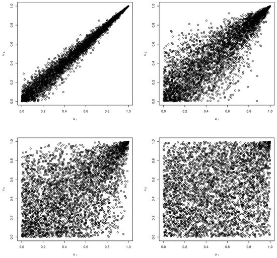
Figure 1 depicts the simulated scatter plots of the copula function $C_{\gamma }$ for varying values of the $\gamma$ parameter.

Figure 1. Scatter plots of the MMG copula (4000 simulation points) for varying values of the $\gamma$ parameter: $\gamma =0.05$ (top left), $\gamma =0.2$ (top right), $\gamma =0.5$ (bottom left), $\gamma =0.8$ (bottom right).

Remark 5.

Copula function (19) is a member of the encompassing class of the Archimedean copulas. Specifically, set

$$\varphi \left(s\right)=\frac{\Gamma (\gamma ,s)}{\Gamma \left(\gamma \right)}\mathit{for}\mathit{all}s\in {\mathbf{R}}_{0,+},$$

and observe that (19) admits the following form, for ${(u_1,\dots ,u_n)}^{\prime }\in {[0,1]}^n$,

$$C_{\varphi }(u_1,\dots ,u_n)=\varphi ({\varphi }^{-1}\left(u_1\right)+\cdots +{\varphi }^{-1}\left(u_n\right)),$$

where $\varphi :[0,\infty )\to [0,1]$ is a legitimate completely monotonic function—known as the Archimedean generator—and ${\varphi }^{-1}$ is its inverse (e.g., McNeil and Nešlehová 2009). The MMG copula therefore enriches the encompassing toolbox of the distinct Archimedean copulas available to researchers and practitioners.

We have already mentioned at the end of Section 2 that the maximum likelihood approach can be used in order to numerically estimate the parameters of the MMG distribution. An alternative way to estimate the parameters is via the two-step copula approach. That is, we first fit the MMG copula to the pseudo uniform samples based on the empirical c.d.f.’s of $X_i$, $i=1,\dots ,n$ and estimate the $\gamma$ parameter (e.g., Embrechts and Hofert 2013; Genest et al. 2011, and references therein), and we then estimate the ${\sigma }_i$ parameters based on the univariate marginal distributions assuming that the $\gamma$ parameter is known. Given the cumbersome form of p.d.f. (8), the copula-based approach is computationally simpler.

Besides the just-mentioned statistical inference, a useful contribution of copulas to the vast literature of multivariate modelling is that they have given rise to a number of indices of dependence that circumvent the known fallacies of the Pearson $\rho$. Such indices of dependence are, e.g., the Kendall $\tau$ and Spearman ${\rho }_S$ measures of rank correlation, and we derive these two in the next subsection in the context of the MMG copula function $C_{\gamma }$.

In the rest of this subsection, we build up the theoretical groundwork necessary for exploring the tail dependence of $C_{\gamma }$. As tail dependence represents the co-movement of extreme risks, it is of particular importance in the era following the financial crisis of 2007–2009. We note in passing that, since the majority of the existing methods for quantifying tail dependence mainly aim at random pairs, we specialize the discussion in this part of the present report to the bivariate case only.

Let $\widehat{C}$ denote the survival copula that corresponds to C, that is $\widehat{C}(u_1,u_2):=u_1+u_2-1+$$C(1-u_1,1-u_2)$, for $u_1,u_2\in [0,1]$. Then the first order lower and upper tail dependence parameters (e.g., Joe 1997) are given by

$$\begin{array}{c}\hfill {\lambda }_L:=\underset{u\downarrow 0}{\lim }\frac{C(u,u)}{u}\mathrm{and}{\lambda }_U:=\underset{u\downarrow 0}{\lim }\frac{\widehat{C}(u,u)}{u},\end{array}$$

(21)

whereas the second order tail dependence parameters (Coles et al. 1999) are given by

$$\begin{array}{c}\hfill {\chi }_L:=\underset{u\downarrow 0}{\lim }\frac{2\log u}{\log C(u,u)}-1\mathrm{and}{\chi }_U:=\underset{u\downarrow 0}{\lim }\frac{2\log u}{\log \widehat{C}(u,u)}-1.\end{array}$$

(22)

Recently, an argument has been put forward that tail dependence measures (21) and (22) may underestimate the extent of the tail dependence inherent in a copula. More specifically, Furman et al. (2015) claim and elucidate with numerous examples that as measures (21) and (22) are computed along the main diagonal $(u,u),u\in [0,1]$, their values are not necessarily maximal when alternative paths in ${[0,1]}^2$ are considered. This motivated the following definitions of the admissible paths and the paths of maximal dependence in ibid.

Definition 2.

A function $\phi :[0,1]\to [0,1]$ is called admissible if it satisfies the following conditions:

(C1) 

$\phi \left(u\right)\in [u^2,1]$ for every $u\in [0,1]$; and

(C2) 

$\phi \left(u\right)$ and $u^2/\phi \left(u\right)$ converge to 0 when $u\downarrow 0$.

Then the path ${(\phi \left(u\right),u^2/\phi \left(u\right))}_{0\le u\le 1}$ is admissible whenever the function φ is admissible. In addition, we denote by $\mathcal{A}$ the set of all admissible functions φ.

Definition 3.

The path(s) ${(\phi \left(u\right),u^2/\phi \left(u\right))}_{0\le u\le 1}$ in $\mathcal{A}$ are called paths of maximal dependence if they maximize the probability

$${\Pi }_{\phi }\left(u\right)=C\left(\phi \left(u\right),u^2/\phi \left(u\right)\right)$$

or, equivalently, the distance function

$$d_{\phi }\left(C,C^{\perp }\right)\left(u\right)=C\left(\phi \left(u\right),u^2/\phi \left(u\right)\right)-C^{\perp }(\phi \left(u\right),u^2/\phi \left(u\right)),$$

where $C^{\perp }$ is the independence copula, i.e., $C^{\perp }(u_1,u_2)=u_1{u}_2$ for all $0\le u_1,u_2\le 1$.

Obviously, the function ${\phi }_0\left(u\right)=u$ is admissible and yields the representation of the diagonal path that serves as a building block for classical indices (21) and (22). For the Archimedean class of copulas, the following property of the maximal dependence path holds. The verification of the condition stated in Lemma 3 below is not trivial, and is carried out for the MMG copula $C_{\gamma }$ in Theorem 6.

Lemma 3 

(Furman et al. 2015). For an Archimedean copula with generator ϕ, if $x\frac{\partial }{\partial x}{\varphi }^{-1}\left(x\right)$ is increasing on $x\in (0,1),$ then the path of maximal dependence coincides with the main diagonal.

The next lemma on a L’Hospital type rule for monotonicity, plays an importantly auxiliary role when deriving the maximal dependence path for $C_{\gamma }$.

Lemma 4 

(Pinelis 2002). Let $-\infty \le a<b\le \infty$, also $g_1$ and $g_2$ be differentiable functions over the interval $(a,b)$. Assume that $g_2^{\prime }\left(s\right)<0$ for $s\in (a,b)$, and ${\lim }_{s\downarrow a}{g}_1\left(s\right)=0$ and ${\lim }_{s\downarrow a}{g}_2\left(s\right)=0$. Then, $g_1/g_2$ is increasing on $(a,b)$ if $g_1^{\prime }/g_2^{\prime }$ is increasing.

Our last result in this subsection implies that measures of tail dependence (21) and (22) are in fact maximal in the context of the MMG copula $C_{\gamma }$.

Theorem 6.

The maximal dependence path of the copula function $C_{\gamma }$ in (19) is diagonal.

4.2. Applications

The next assertion reports the Kendall tau and Spearman rho rank correlations, implied by the MMG copula (19). The hypergeometric function plays a pivotal role in deriving the Spearman rho correlation in the following proposition, and it is given in Gradshteyn and Ryzhik (2014)

$$\begin{array}{c}\hfill {}_{q+1}{F}_q(a_1,\dots ,a_{q+1};b_1,\dots ,b_q;z)=\sum _{k=0}^{\infty }\frac{{⟨a_1⟩}_k,\dots ,{⟨a_{q+1}⟩}_k}{{⟨b_1⟩}_k,\dots ,{⟨b_q⟩}_k}\frac{z^k}{k!}.\end{array}$$

(23)

For $a_1,\dots ,a_{q+1}$ all positive, and these are the cases of interest in the present report. The radius of convergence of the series is the open disk $\left|z\right|<1$. On the boundary $\left|z\right|=1$, the series converges absolutely if $d=b_1+\cdots +b_q-a_1-\cdots -a_{q+1}>0$, and it converges except at $z=1$ if $0\ge d>-1$.

Proposition 5.

For the copula $C_{\gamma }$, the Kendall τ rank correlation is given by

$$\tau \left(C_{\gamma }\right)=1-\frac{2\Gamma (\gamma +1/2)}{\sqrt{\pi }\Gamma \left(\gamma \right)},$$

and the Spearman ${\rho }_S$ rank correlation is given by

$${\rho }_S\left(C_{\gamma }\right)=6\left(\frac{8^{-\gamma }\Gamma \left(3\gamma \right)}{\Gamma (\gamma +1)\Gamma \left(2\gamma \right)}{}_2{F}_1(1,3\gamma ;2\gamma +1;1/2)-1/2\right).$$

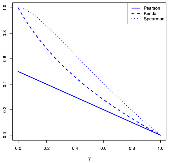
Figure 2 depicts the values for the Pearson $\rho$, Kendall $\tau$ and Spearman ${\rho }_S$ indices of correlation with varying $\gamma \in (0,1)$. The figure confirms that, while the Pearson $\rho$ does not attain all values in $[0,1]$ for the MMG/G-MBRM distribution, the other two indices are able to achieve this goal.

Figure 2. The plot of the Pearson rho, Kendall tau, and Spearman rho measures of correlation for varying values of $\gamma \in (0,1)$.

Proposition 6.

Assume that $\mathbf{X}\sim G{a}_n^{\times }(\gamma ,\sigma )$ has copula $C_{\gamma }$, the lower maximal tail dependence of $C_{\gamma }$ is

$${\lambda }_L\left(C_{\gamma }\right)={\chi }_L\left(C_{\gamma }\right)=0.$$

The upper maximal tail dependence of $C_{\gamma }$ is

$${\lambda }_U\left(C_{\gamma }\right)=2-2^{\gamma },\mathit{and}{\chi }_U\left(C_{\gamma }\right)=1.$$

Proposition 6 readily implies—recall to this end that the copula $C_{\gamma }$ is in fact a survival copula (by construction)—that the coordinates of $\mathbf{X}\sim G{a}_n^{\times }(\gamma ,\sigma )$ are asymptotically dependent in the lower tail, but independent in the upper tail. Speaking bluntly, this means that $\mathbf{X}$ is more likely to take smaller values simultaneously, but less likely to form a cluster of large values. This conforms to the already made intuitive observation that the copula $C_{\gamma }$ can serve as a reflected variant of the well-studied Clayton copula.

5. Conclusions

In the present report, we have systematically studied a class of multivariate multiplicative gamma distributions. We have demonstrated that the MMG distribution admits a very meaningful background risk model representation, where the interdependencies among risks are implied by a common systematic risk factor. Moreover, we have shown that the MMG distribution enjoys a remarkable level of analytical tractability, that is, the risk r.v.’s distributed MMG are straightforward to simulate, easy to aggregate and take maxima, closed under minima, and have attractive dependence and tail dependence characteristics. In view of the above, we think that the potential applications of the MMG distribution in actuarial science are vast, and we hope to draw the attention of the community to this class of distributions. In fact, reduced forms of the proposed MMG distribution have been recently heuristically adopted in the actuarial literature to model a variety of dependent insurance risks (e.g., Sarabia et al. 2018, also, Albrecher et al. 2011).

References

- Akkouchi, Mohamed. 2008. On the convolution of exponential distributions. Journal of the Chungcheong Mathematical Society 21: 501–10. [Google Scholar]
- Albrecher, Hansjörg, Corina Constantinescu, and Stephane Loisel. 2011. Explicit ruin formulas for models with dependence among risks. Insurance: Mathematics and Economics 48: 265–70. [Google Scholar] [CrossRef] [Scilit]
- Asimit, Alexandru V., Raluca Vernic, and Ricardas Zitikis. 2016. Background risk models and stepwise portfolio construction. Methodology and Computing in Applied Probability 18: 805–27. [Google Scholar] [CrossRef] [Scilit]
- Avanzi, Benjamin, Greg Taylor, Phuong Anh Vu, and Bernard Wong. 2016. Stochastic loss reserving with dependence: A flexible multivariate Tweedie approach. Insurance: Mathematics and Economics 71: 63–78. [Google Scholar] [CrossRef] [Scilit]
- Bahraoui, Zuhair, Catalina Bolancé, Elena Pelican, and Raluca Vernic. 2015. On the bivariate Sarmanov distribution and copula. An application on insurance data using truncated marginal distributions. Statistics & Operations Research Transactions 39: 209–30. [Google Scholar]
- Balakrishnan, Narayanaswamy, and Miroslav M. Ristić. 2016. Multivariate families of gamma-generated distributions with finite or infinite support above or below the diagonal. Journal of Multivariate Analysis 143: 194–207. [Google Scholar] [CrossRef] [Scilit]
- Bingham, Nicholas H., Charles M. Goldie, and Jef L. Teugels. 1987. Regular Variation. Cambridge: Cambridge University Press. [Google Scholar]
- Coles, Stuart, Janet Heffernan, and Jonathan Tawn. 1999. Dependence measures for extreme value analyses. Extremes 2: 339–65. [Google Scholar] [CrossRef] [Scilit]
- Cossette, Hélène, Etienne Marceau, Itre Mtalai, and Déry Veilleux. 2018. Dependent risk models with Archimedean copulas: A computational strategy based on common mixtures and applications. Insurance: Mathematics and Economics 78: 53–71. [Google Scholar] [CrossRef] [Scilit]
- Das, Sanjiv R., Darrell Duffie, Nikunj Kapadia, and Leandro Saita. 2007. Common failings: How corporate defaults are correlated. Journal of Finance 62: 93–117. [Google Scholar] [CrossRef] [Scilit]
- Dornheim, Harald, and Vytaras Brazauskas. 2007. Robust and efficient methods for credibility when claims are approximately gamma distributed. North American Actuarial Journal 11: 138–58. [Google Scholar] [CrossRef] [Scilit]
- Embrechts, Paul, and Marius Hofert. 2013. Statistical inference for copulas in high dimensions: A simulation study. ASTIN Bulletin 43: 81–95. [Google Scholar] [CrossRef] [Scilit]
- Feller, William. 1968. An Introduction to Probability Theory and Its Applications. New York: Wiley. [Google Scholar]
- Frank, Günter, Harris Schlesinger, and Richard C. Stapleton. 2006. Multiplicative background risk. Management Science 52: 146–53. [Google Scholar] [CrossRef] [Scilit]
- Furman, Edward, Daniel Hackmann, and Alexey Kuznetsov. 2018. On Log-Normal Convolutions: An Analytical-Numerical Method with Applications to Economic Capital Determination. Technical Report. Haifa: Actuarial Research Center—University of Haifa. [Google Scholar]
- Furman, Edward, and Zinoviy Landsman. 2005. Risk capital decomposition for a multivariate dependent gamma portfolio. Insurance: Mathematics and Economics 37: 635–49. [Google Scholar] [CrossRef] [Scilit]
- Furman, Edward, Jianxi Su, and Ričardas Zitikis. 2015. Paths and indices of maximal tail dependence. ASTIN Bulletin 45: 661–78. [Google Scholar] [CrossRef] [Scilit]
- Genest, Christian, Johanna Nešlehová, and Johanna Ziegel. 2011. Inference in multivariate archimedean copula models. Test 20: 223–56. [Google Scholar] [CrossRef] [Scilit]
- Gollier, Christian, and John W. Pratt. 1996. Risk vulnerability and the tempering effect of background risk. Econometrica 64: 1109–23. [Google Scholar] [CrossRef] [Scilit]
- Gradshteyn, Izrail Solomonovich, and Iosif Moiseevich Ryzhik. 2014. Table of Integrals, Series, and Products, 8th ed. New York: Academic Press. [Google Scholar] [CrossRef] [Scilit]
- Hürlimann, Werner. 2001. Analytical evaluation of economic risk capital for portfolios of gamma risks. ASTIN Bulletin 31: 107–22. [Google Scholar] [CrossRef] [Scilit]
- Joe, Harry. 1997. Multivariate Models and Dependence Concepts. London: Chapman and Hall. [Google Scholar]
- Klugman, Stuart A., Harry H. Panjer, and Gordon E. Willmot. 2012. Loss Models: From Data to Decisions, 4th ed. Hoboken: Wiley. [Google Scholar]
- Kotz, Samuel, Narayanaswamy Balakrishnan, and Norman L. Johnson. 2000. Continuous Multivariate Distributions: Models and Applications. New York: Wiley. [Google Scholar]
- Kunz, Karls S. 1956. High accuracy quadrature formulas from divided differences with repeated arguments. Mathematical Tables and Other Aids to Computation 10: 87–90. [Google Scholar] [CrossRef] [Scilit]
- Mathai, Arak M., and Panagis G. Moschopoulos. 1991. On a multivariate gamma. Journal of Multivariate Analysis 39: 135–53. [Google Scholar] [CrossRef] [Scilit]
- McNeil, Alexander J., and Johanna Nešlehová. 2009. Multivariate Archimedean copulas, d-monotone functions and l1-norm symmetric distributions. Annals of Statistics 37: 3059–97. [Google Scholar] [CrossRef] [Scilit]
- Milne-Thomson, Louis Melville. 2000. The Calculus of Finite Differences. Rhode Island: American Mathematical Society. [Google Scholar]
- Moschopoulos, Peter G. 1985. The distribution of the sum of independent gamma random variables. Annals of the Institute of Statistical Mathematics 37: 541–44. [Google Scholar] [CrossRef] [Scilit]
- Pinelis, Iosif. 2002. L’Hospital type rules for monotonicity: Applications to probability inequalities for sums of bounded random variables. Journal of Inequalities in Pure and Applied Mathematics 3: 7. [Google Scholar]
- Provost, Serge. 1989. On sums of independent gamma eandom yariames. Statistics 20: 583–91. [Google Scholar] [CrossRef] [Scilit]
- Sarabia, José María, Emilio Gómez-Déniz, Faustino Prieto, and Vanesa Jordá. 2018. Aggregation of dependent risks in mixtures of exponential distributions and extensions. ASTIN Bulletin. [Google Scholar] [CrossRef] [Scilit]
- Srivastava, Hari M., and Per Wennerberg Karlsson. 1985. Multiple Gaussian Hypergeometric Series. Chichester: Ellis Horwood. [Google Scholar]
- Su, Jianxi, and Edward Furman. 2017a. A form of multivariate Pareto distribution with applications to financial risk measurement. ASTIN Bulletin 47: 331–57. [Google Scholar] [CrossRef] [Scilit]
- Su, Jianxi, and Edward Furman. 2017b. Multiple risk factor dependence structures: Distributional properties. Insurance: Mathematics and Economics 76: 56–68. [Google Scholar] [CrossRef] [Scilit]
- Su, Jianxi, and Lei Hua. 2017. A general approach to full-range tail dependence copulas. Insurance: Mathematics and Economics 77: 49–64. [Google Scholar] [CrossRef] [Scilit]
- Temme, Nico. 1996. Special Functions: An Introduction to the Classical Functions of Mathematical Physics. New York: Wiley. [Google Scholar]
- Zhou, Ming, Jan Dhaene, and Jing Yao. 2018. An approximation method for risk aggregations and capital allocation rules based on additive risk factor models. Insurance: Mathematics and Economics 79: 92–100. [Google Scholar] [CrossRef] [Scilit]
© 2018 by the authors. Licensee MDPI, Basel, Switzerland. This article is an open access article distributed under the terms and conditions of the Creative Commons Attribution (CC BY) license (http://creativecommons.org/licenses/by/4.0/).