Article

Robust Estimation of Value-at-Risk through Distribution-Free and Parametric Approaches Using the Joint Severity and Frequency Model: Applications in Financial, Actuarial, and Natural Calamities Domains

Systems Engineering & Operations Research, George Mason University, Fairfax, VA 22030, USA
*
Author to whom correspondence should be addressed.
Risks 2017, 5(3), 41; https://doi.org/10.3390/risks5030041
Submission received: 31 May 2017 / Revised: 5 July 2017 / Accepted: 21 July 2017 / Published: 26 July 2017

Abstract

:
Value-at-Risk (VaR) is a well-accepted risk metric in modern quantitative risk management (QRM). The classical Monte Carlo simulation (MCS) approach, denoted henceforth as the classical approach, assumes the independence of loss severity and loss frequency. In practice, this assumption does not always hold true. Through mathematical analyses, we show that the classical approach is prone to significant biases when the independence assumption is violated. This is also corroborated by studying both simulated and real-world datasets. To overcome the limitations and to more accurately estimate VaR, we develop and implement the following two approaches for VaR estimation: the data-driven partitioning of frequency and severity (DPFS) using clustering analysis, and copula-based parametric modeling of frequency and severity (CPFS). These two approaches are verified using simulation experiments on synthetic data and validated on five publicly available datasets from diverse domains; namely, the financial indices data of Standard & Poor’s 500 and the Dow Jones industrial average, chemical loss spills as tracked by the US Coast Guard, Australian automobile accidents, and US hurricane losses. The classical approach estimates VaR inaccurately for 80% of the simulated data sets and for 60% of the real-world data sets studied in this work. Both the DPFS and the CPFS methodologies attain VaR estimates within 99% bootstrap confidence interval bounds for both simulated and real-world data. We provide a process flowchart for risk practitioners describing the steps for using the DPFS versus the CPFS methodology for VaR estimation in real-world loss datasets.

1. Introduction

Research activities in quantitative risk management (QRM) have been steadily growing, due to its capability to analyze, quantify, and mitigate risks associated with various events that cause losses. Three types of quantitatively measurable risks are well understood: market risk, credit risk, and operational risk. These risks have established definitions and processes for quantification (Hull 2015). To manage risks, regulatory agencies require financial institutions to hold economic capital (EC) to absorb potential losses (Balthazar 2006). The key question of interest concerns the amount of capital a financial institution should hold to absorb a certain level (percentage) of loss over a certain time frame. Value-at-Risk (Guharay 2016; Böcker and Klüppelberg 2005; Böcker and Sprittulla 2006; Guharay et al. 2016; Panjer 2006; Aue and Kalkbrener 2006; Wipplinger 2007; OpRisk Advisory and Towers Perrin 2010; Guharay and Chang 2015; Gomes-Gonçalves and Gzyl 2014; Rachev et al. 2006; Embrechts et al. 2015; Li et al. 2014), denoted as VaR, is a quantitative risk metric used to answer this key question. Developing methods for the robust estimation of VaR for a generalized setting is a problem which is currently of interest in QRM. In the context of risk analysis, this paper develops and implements two distinct statistical approaches for VaR estimates covering different types of relationships, including both independence and dependence, between loss severity and loss frequency. We have tested this methodology through verification via simulation and validation using publicly available real-world datasets. We have demonstrated that this approach outperforms the classical approach (Aue and Kalkbrener 2006; OpRisk Advisory and Towers Perrin 2010; Gomes-Gonçalves and Gzyl 2014; Rachev et al. 2006; Li et al. 2014), which assumes independence between loss frequency and loss severity. The three key contributions of this work are highlighted below:
(a)
We provide mathematical analyses for scenarios in which the assumption of the independence of frequency and severity does not hold, and show that the classical approach incurs large and systematic errors in the estimation of VaR, thus exposing a limitation in the approach.
(b)
We propose two methods that do not assume the independence of frequency and severity and subsequently provide robust estimates for VaR for diverse QRM applications. The first method, the data-driven partitioning of frequency and severity (DPFS), is non-parametric. It performs a clustering analysis to separate the loss data into clusters in which the independence assumption (approximately) holds. The second method, copula-based parametric modeling of frequency and severity (CPFS), parametrically models the relationship between loss frequency and loss severity using a statistical machinery known as a copula. We extend CPFS to the recently developed Gaussian mixture copula (Bilgrau et al. 2016; Wu et al. 2014; Bayestehtashk and Shafran 2015) along with the classical Gaussian and students-t copula in order to deal with instances of nonlinear, linear, and tail dependencies between loss frequency and loss severity.
(c)
We investigate the performance of the classical and DPFS and CPFS methodologies using both simulation experiments and publicly available real-world datasets from a diverse range of application domains; namely, financial market losses (Data available from Yahoo Finance 2017), chemical spills handled by the US Coast Guard (Data available at National Response Center 1990), automobile accidents (Charpentier 2014), and US hurricane losses (Charpentier 2014). The use of publicly available data sets this work distinctly apart from the majority of the empirical research into modern QRM which uses proprietary data (Aue and Kalkbrener 2006; OpRisk Advisory and Towers Perrin 2010; Gomes-Gonçalves and Gzyl 2014; Rachev et al. 2006; Embrechts et al. 2015; Li et al. 2014). Tests using simulations and real-world data demonstrate the merit of the two statistical approaches. A flowchart is provided for risk practitioners to select a methodology for VaR estimation depending on the loss data characteristics.
We give a brief background on Value-at-Risk in Section 2, followed by a description of the methodology in Section 3. Next, we present both simulated data (for verification) and real-world data (for validation) in Section 4, followed by the results in Section 5. Section 6 compares and discusses the performances of the methodologies. Conclusions are narrated in Section 7, in which we summarize our primary findings from this work and discuss areas for future research. Finally, in Appendix A and Appendix B, we describe, respectively, the theoretical calculations and simulation methodology in detail.

2. Background on Value-at-Risk

For a pre-specified quantile κ (0, 1) and time horizon T, the VaRκ,T is defined as the smallest number s such that the probability of the aggregated loss S exceeding s is less than κ for time horizon T:
VaR κ , T ( S ) = inf { s R : Pr ( S > s ) κ }
We use F S ( s ) to denote the cumulative distribution function (CDF) of the aggregated loss S. An alternative metric is the conditional VaR (CVaR) or the expected shortfall (ES), which measures the average loss amount exceeding a given VaR. Detailed descriptions and the backgrounds of different risk measures can be found in Embrechts et al. (2015). In addition to operational risk, this measure has applications in the market risk and credit risk domains (Embrechts and Hofert 2014; Dias 2013; Andersson et al. 2001). Both gains and losses are included for market risk, while the probability of default is the main quantity of interest in calculating VaR for credit risk. Robust VaR measures have been developed to estimate the predictive distributions of generalized auto-regressive conditional heteroskedasticity (GARCH) models (Mancini and Trojani 2011). This method uses a semiparametric bootstrap to obtain robust VaR predictions in the market risk contexts in which a GARCH model is applicable. The operational risk framework uses a generalized approach of looking at the statistical characteristics of the losses based on their magnitude (severity) and the number of occurrences (frequency). This joint severity-frequency model is defined following the guidelines from the Basel committee on banking supervision (BCBS) (Balthazar 2006). The aggregated loss, S, is modeled as a random sum in the following manner:
S = i = 0 N ( T ) L i , L i ~ i . i . d . F γ .
The loss magnitudes (severity) are described by the independent and identically distributed (i.i.d.) sequence of continuous random variables {Li} with a CDF of Fγ, which is assumed to belong to a parametric family of distributions, γ in Equation (2). The discrete counting process N(T) describes the frequency of loss events as a function of the total time T. In Equation (2), there is an implicit assumption of independence between severity and frequency. This assumption allows one to estimate a univariate discrete probability distribution for the frequency and a univariate continuous probability distribution for the severity from the loss data. In modern QRM, the frequency is typically modeled using the Poisson (Pois) distribution, where the sample mean and the sample variance are equal (Panjer 2006). Since the magnitudes of losses are always non-negative, the severity is modeled using continuous distributions with positive support, such as log-normal (LN), Type XII Burr, generalized Pareto, Weibull, and log-normal-gamma distributions (OpRisk Advisory and Towers Perrin 2010). Recent work has also explored the use of the extreme value theory for modeling loss data depending on covariates (Chavez-Demoulin et al. 2016). Statistical goodness-of-fit (GoF) tests can be used to determine the adequacy of fit and help in selecting a distribution model to use for loss severity and loss frequency. Once the frequency and severity distribution models are estimated from the loss data, one can use the Monte Carlo simulation (MCS) to first generate the number of loss events and then, independently, the severity of each loss event. Then, the individual loss severities are summed up for the loss events which occurred in the fixed time horizon of interest T, to obtain a sample from the aggregate loss distribution. The primary reason for using MCS is that there is no closed-form expression for the CDF given in Equation (2). In other words, as there is no generalized closed form analytical expression for the aggregate loss S, VaR can be only estimated using a numerical procedure such as MCS. We refer to the aforementioned approach as the classical VaR estimation process for a loss model. A graphical representation of the process is shown in Figure 1.

3. Methodology

In this section, we first present a mathematical analysis of the classical VaR estimation approach, in which the loss data consists of the correlated frequency and severity. This analytical setup provides motivation as to why one should expand upon the classical method for VaR estimation and in what type of situations the classical method is not reliable for estimating VaR. We then provide the details of the proposed two statistical methodologies; namely, the non-parametric DPFS and the parametric CPFS method for estimating VaR.

3.1. VaR Estimation Bias using the Classical Method

The assumption of frequency and severity independence enables the classical approach to decompose the estimation of VaR. This decomposition involves the estimation of the marginal densities of loss severity and loss frequency from the aggregated loss distribution. When this assumption does not hold, the reliability of the classical approach in producing accurate VaR estimates is unknown. To test this hypothesis, we analyze the estimation of VaR for two scenarios.
Suppose that the data-generating process (DGP) produces losses as a mixture of two independent compound Poisson processes SX, SY with loss severity components X, Y and loss frequency components M, N. Suppose both X and Y follow a log-normal distribution, i.e., X ~ LN(μ, σ), Y ~ LN(μ/k, σ), and that the loss frequencies follow a Poisson distribution with M ~ Pois(λ/l) and N ~ Pois(λ), where k, l are fixed constants with a magnitude greater than one. The two compound Poisson processes are represented as the following:
S X = j = 1 M X j , S Y = i = 1 N Y i ,
where SX represents the “high severity/low frequency” regime and SY represents the “low severity/high frequency” regime. The compound Poisson process for the aggregated loss SZ is the following:
S Z = S X + S Y ,
where the individual loss event Z comes from the DGP of loss severities X and Y. Let us now define probability p, as the chance that the loss Z comes from the loss severity X. This is defined as the following:
Z = { X   with   probability   p = λ l λ l + λ = 1 l + 1 Y   with   probability   1 p = l l + 1
It is important to note that at this stage it is not known whether an individual loss event is a realization from either severity distribution X or severity distribution Y. The frequency and severity of the loss events Z and its sum Sz are the only observable quantities. The variables X, M, Y, and N are all independent. Let Pr{ S Z z} = F( S Z ) be the CDF of S Z and let VaRκ( S Z ) = F−1( S Z |κ) be defined for a right tail quantile κ (we drop the time horizon T to simplify the notation since T is usually 1 month/year); while individual loss events Z’s are still i.i.d., the frequency and severity distributions are no longer independent. For example, if a particular time period has a much higher frequency than average, it implies that most loss events are more likely to have come from the S Y process, instead of S X , and thus consist of smaller loss magnitudes.
The classical approach independently fits marginal distributions to the loss frequency and loss severity based on the observations of the individual loss events Z, then estimates VaR for a quantile κ using MCS. We denote this as VaR κ ( C ) . Since the underlying independence assumption is not valid under the current setting, we calculate VaR κ ( C ) and check the value with respect to the true VaR, which we denote as VaR κ ( * ) . We analyze how VaR κ ( C ) differs, if at all, from the VaR κ ( * ) for the following two cases (we fix 0 < σ < 1 ) :
  • Case (I): μ = O ( e λ ) . This corresponds to a regime in which the mean severity dominates the frequency; i.e., a relatively small number of loss events but each loss is large (in magnitude).
  • Case (II): λ = O ( e e μ ) . This corresponds to a regime in which frequency dominates severity; i.e., a large number of small (in magnitude) losses.
It is important to note that p, being the proportion of losses coming from X, is neither 1 nor 0 in both cases. This is because p = 1 means that Z consists solely of X. This is not the setup for Case (I): the setup here is that the mean severity (μ) dominates the mean frequency (λ) and vice versa for Case (II). It is important to note that p is not correlated with the size of the losses, but on average p = 1/(l+1). The reason for setting this mathematical framework is to diagnose the effect of the assumption of independence among severity and frequency in the two extreme cases of high degrees of correlation (i.e., functional dependence). These two cases examine the “high severity/low frequency” region (Case (I)) and the “high frequency/low severity” region (Case (II)). Previous literature (Guharay and Chang 2015; Gomes-Gonçalves and Gzyl 2014) has shown that the severity process dominates the final VaR estimate over a frequency when both are of similar magnitudes. In order to ensure that the frequency is the dominating factor in the VaR estimation process, we use a double exponential relationship of mean frequency dominating the mean severity in Case (II). We have the following proposition on the systematic bias in VaR κ ( C ) for these two cases.
Proposition 1.
Suppose that the loss severity distribution is log-normal and the loss frequency follows a Poisson distribution. As κ 1 , V a R κ ( C ) < V a R κ ( * ) in Case (I) and V a R κ ( C ) > V a R κ ( * ) in Case (II).
Proposition 1 formally establishes the conjecture that the classical approach incorrectly estimates the VaR when the frequency and severity independence assumption does not hold. Specifically, the classical approach systematically underestimates VaR for Case (I) and overestimates VaR for Case (II). The proof is given in Appendix A. The argument uses the Fenton–Wilkinson approximation (Mehta et al. 2007) to calculate VaR κ ( C ) , and compare it to VaR κ ( * ) . VaR κ ( * ) is computed using the single-loss VaR approximation (Böcker and Klüppelberg 2005) for Case (I) and the mean-adjusted single-loss VaR approximation (Böcker and Sprittulla 2006) using the conditions specified on μ and λ . These conditions imply that either S X (Case I) or S Y (Case II) dominates the other, and thus VaR κ ( * ) can be calculated using an analytical approximation.

3.2. Non-Parametric DPFS Method for VaR Estimation

The two-component mixture regime studied in Section 3.1 can be extended to general cases with K components, where K is an arbitrary positive integer, and can model the relationship between severity and frequency in the aggregated loss process. K may be equal to 1 when the independence assumption holds. In Wang et al. (2016), different banking business lines were treated as components within which the independence assumption holds, and the aggregate VaR estimate was computed using mutual information. However, in general settings, one may not be able to identify such pre-defined components to work with, and it is also not clear if the independence assumption holds true within each component. In this section, we propose a non-parametric approach that can identify such components from data and model dependencies in which finite partitions between loss frequency and loss severity are possible.
The premise of the DPFS is to identify the types of relationships between the loss frequency and loss severity through a non-parametric clustering analysis. It partitions the data into clusters within which the independence assumption between loss frequency and loss severity approximately holds true. The term “distribution-free” refers to the overall goal of using a non-parametric approach to determine the relationship, if any, between loss frequency and loss severity. The marginal severity and frequency distributions can be estimated reliably for each cluster and used to estimate VaR. This clustering framework allows for both paradigms of independence and dependence between frequency and severity. We use the K-means algorithm (MacKay 2003; Martinez and Martinez 2007; Kaufman and Rousseeuw 2009). The number of clusters (K) is determined using the Silhouette Statistic (SS) (Kaufman and Rousseeuw 2009; Xu et al. 2012). SS provides a heuristic method for measuring how well each data point lies within a cluster object. This is one of several metrics (MacKay 2003; Martinez and Martinez 2007; Kaufman and Rousseeuw 2009; Xu et al. 2012) which can be used to determine the optimal number of clusters (K).
We propose two different methods to partition the loss frequency and loss severity components under the aggregated loss model. Method I performs a two-dimensional clustering analysis on the mean severity and frequency; this is computed for all individual loss events occurring during one unit of the time horizon of interest (e.g., monthly/annually). For instance, for loss data calculated for a monthly horizon, we first group individual losses by the months of their occurrence. We compute the mean severity of all losses and then count the frequency of loss events for each month. DPFS Method I then uses the K-means algorithm to cluster these monthly data points into K clusters. The optimal value of K is determined using the SS. Since the independence of frequency and severity holds approximately true within each cluster, the marginal severity and frequency distributions are fit for the loss events belonging to each cluster.
DPFS Method II clusters data solely based on the severity of individual loss events. Suppose that the loss severity consists of daily loss data, while the loss frequency consists of counts of the number of losses that occurs in a month. Assume that there are N total daily loss data and m total months (where by definition m < N). Suppose that the severity only data (i.e., losses L1,...,LN) are split into K groups, where the optimal number K is determined by the SS. For each month from 1 to m, we compute the frequency in each group; for instance, ni for i = 1,2,...K. The implied frequency for group i is the average of ni taken over all m months. The reason that the term “implied frequency” is used here is because the frequency is calculated after the K-means is computed on the loss severity portion. This frequency is implied from the K-means loss severity only. Once this clustering is completed and the implied frequencies are determined, the independence assumption holds true within each cluster. Once all loss events have been grouped into K clusters, we compute the implied frequency of each cluster and use this information in the VaR estimation. We fit the marginal distribution for the loss frequency and loss severity and use a simulation for VaR estimation. To summarize both Methods (I) and (II), we describe the DPFS procedure in Algorithm 1.
Algorithm 1 Data-driving partitioning of frequency and severity (DPFS) (Methods I and II) VaR estimation
  • Cluster loss data by either mean severity/frequency (Method I) or severity only (Method II) into K clusters.
  • Estimate the marginal severity and frequency distributions for each cluster (K) using the classical approach, as the independence of severity and frequency holds approximately true within each cluster.
  • Use MCS to estimate aggregate losses for each cluster using the marginal severity and frequency distributions estimated in Step 2.
  • The overall VaR is calculated through concatenating the individual losses from each cluster (K)

3.3. Parametric CPFS Method for VaR Estimation

Copula is a statistical method for modeling probabilistic dependence among random variables. Copulas have been used extensively in various applications in QRM (Nelsen 2007; Tewari et al. 2011; Sklar 1959; Kojadinovic and Yan 2010; Panchenko 2005; Kojadinovic and Yan 2011; Kole et al. 2007). In this paper, we propose to use the copula model in a generalized QRM setting where the losses are broken down in the joint severity/frequency model.
A q-dimensional copula C: [0, 1]q→[0, 1] is a multivariate CDF function with marginal densities being a uniform distribution. The connection between copulas and the joint distribution of multivariate random variables is established by Sklar’s Theorem (Kaufman and Rousseeuw 2009), which states that the copula for q random variables X1, ..., Xq can be expressed as the following:
C ( u 1 , ... , u q ) = F ( F 1 1 ( u 1 ) , ... , F 1 q ( u q ) ) ,
where F is the joint CDF of (X1, ..., Xq), F 1 1 , , F q 1 are the inverse of marginal CDFs and ( u 1 , ... , u q ) are i.i.d. uniform random variables with a support of (0, 1). In other words, a joint probability distribution function of any set of dependent random variables can be specified by their given marginal distributions and a chosen copula function. Well-known copula functions include Gaussian, Archimedean, and the student’s t (Nelsen 2007).
In this study, we choose the Gaussian copula and the student’s t-copula (t-copula) for their ease of interpretation and their general applicability in various QRM domains. The Gaussian copula can be expressed as the following for a specified correlation matrix Σ:
C Gaussian ( u 1 , ... , u q   |   Σ ) = Φ Σ ( Φ 1 ( u 1 ) , ... , Φ 1 ( u q ) ) ,
where Φ(·) is the standard normal CDF and ΦΣ(·) is the CDF of a multivariate normal with a zero mean vector and a covariance matrix of Σ. The t-copula is defined for a specified correlation matrix Σ and ν degrees of freedom as the following:
C t ( u 1 , ... , u q   |   Σ , ν ) = t ν , Σ ( t ν 1 ( u 1 ) , ... , t ν 1 ( u q ) ) ,
where t ν ( · ) is the CDF of a student’s t distribution, with a degree of freedom ν , and t ν , Σ ( · ) is the CDF of a multivariate t distribution with a covariance matrix of Σ and ν degrees of freedom.
In addition to the standard Gaussian/t-copulas, we also apply the recently developed Gaussian mixture copula model (GMCM). GMCM extends beyond the linear relationship between frequency and severity as detected by the Gaussian/t-copula. The mathematical formulation assumes an m-component Gaussian mixture model. The technical details are presented in Kojadinovic and Yan (2010) and Panchenko (2005). Empirical GoF tests (Panchenko 2005; Kojadinovic and Yan 2011) are used to validate the model.
Gaussian copulas can model linear dependencies using the Pearson’s correlation coefficient. The student’s t-copula can capture dependencies in the tail region without sacrificing flexibility to model dependence in the body (Kole et al. 2007). The GMCM offers more flexibility than the Gaussian copula, as the Gaussian copula is a special case (m = 1). The GMCM can detect clusters of loss data points with different linear correlations.
CPFS models the relationship between frequency and severity by estimating a copula model for the statistical parameters for loss frequency and loss severity models. The fundamental premise is that the triplets (λi, µi, σi) for all time periods i = 1, 2,…, m are i.i.d. realizations from a random vector (λ, µ, σ). We use the copula model to estimate the joint density of the severity and frequency. To illustrate this procedure, let us consider a loss data set which is aggregated monthly and has m months. For each month i = 1, 2,…, m, we fit the severity of the losses occurring in this month by LN( μ i , σ i ) (other parametric severity loss distributions can be used too), and fit the loss frequency by Pois( λ i ) using a maximum likelihood estimation. Thus, for month i, there will be a 3-parameter triplet ( λ i , μ i , σ i ) estimate. The strength of this approach is that it can model a continuous relationship between severity and frequency, as opposed to a discrete relationship as dictated by the DPFS partition number, K, from the clustering approach. The CPFS method is described in Algorithm 2 below.
Algorithm 2 Copula-based parametric modeling of frequency and severity (CPFS) VaR estimation
  • Estimate triplets ( λ ^ i , μ ^ i , σ ^ i ) for i = 1, 2,…, m time periods for a specified parametric severity model and frequency model using the maximum likelihood method.
  • Fit a copula model C ( λ , μ , σ ) to ( λ ^ i , μ ^ i , σ ^ i ) for i = 1,2,…,m.
  • For n = 1, 2, …, N (simulation size), do the following:
    (a)
    Randomly draw an i.i.d. realization ( λ n ˜ , μ n ˜ , σ n ˜ ) from the estimated joint probability density function F ( λ , μ , σ ) .
    (b)
    Follow the classical approach to generate the aggregated loss S n .
  • Sort S n such that S [ 1 ] S [ 2 ] S [ N ] . Return the appropriate quantile for VaR estimate.
The primary reason that we decompose the CPFS approach into the empirical marginal for the loss severity and loss frequency parameters of interest is due to the fact that the data-generating process inherently consists of finite time horizons. This is because the VaR metric is calculated on a fixed time horizon (which is known a priori). The CPFS approach is analogous to a hierarchical modeling paradigm where the parameters of the frequency and severity distribution (i.e., (λ, µ, σ)) are treated as random, and we are estimating their joint probability density accordingly.

4. Simulated and Real-World Data

The majority of the research publications which use real-world data in modern QRM rely on proprietary data (Aue and Kalkbrener 2006; OpRisk Advisory and Towers Perrin 2010; Gomes-Gonçalves and Gzyl 2014; Rachev et al. 2006; Embrechts et al. 2015; Li et al. 2014). In some rare cases, the data cited is available only in loss data exchanges where users must pay a fee or donate their own specialized loss data in order to access and analyze the data (Aue and Kalkbrener 2006; Gomes-Gonçalves and Gzyl 2014; Rachev et al. 2006; Li et al. 2014). Contrary to the prior approaches, all of the empirical analysis in this paper consists of data freely available to the general public. We first discuss five simulated data sets created using five distinct scenarios for verification purposes in Section 4.1. We then describe the real-world data sets in Section 4.2.

4.1. Simulated Data for Verification

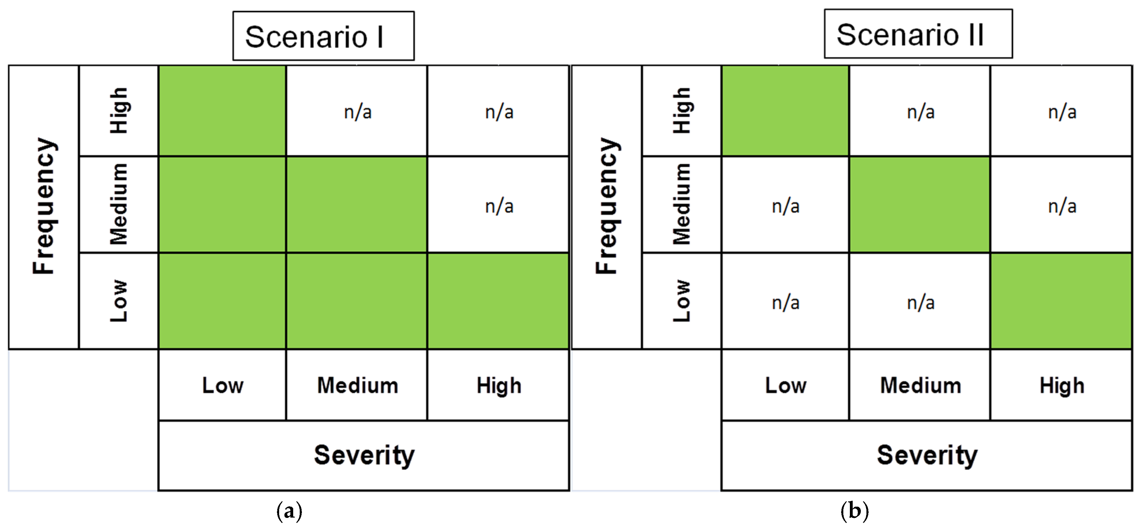
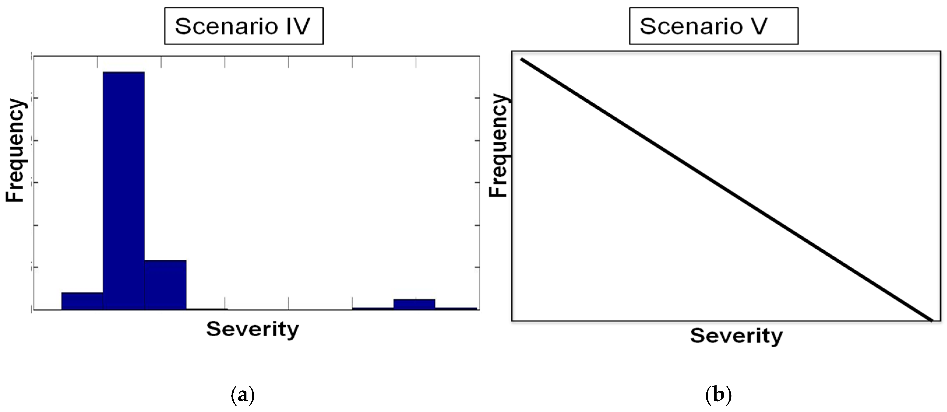
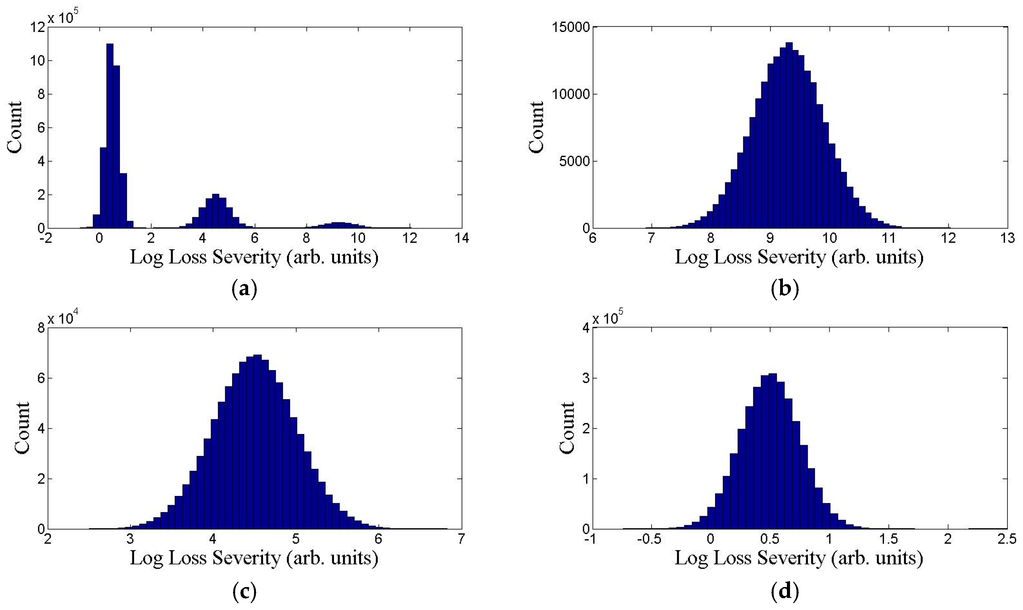
Five distinct scenarios are created to verify the methodologies; namely, the DPFS and CPFS in a controlled experimental environment, in which the true relationship between frequency and severity is known a priori. In all scenarios, we generate the loss severity from a logn-ormal distribution and the loss frequency from a Poisson distribution. Four scenarios—namely, Scenarios (I, II, IV, and V)—are designed to violate the assumption of independence between loss frequency and loss severity, while Scenario (III) satisfies the independence assumption. Scenario (I) and Scenario (II) partition the frequency and severity into high/medium/low regions. For Scenario (I), there is a one-to-many relationship between frequency and severity. In Scenario (II), there is a one-to-one relationship between frequency and severity. An illustration representing the relationship between the partitioning of severity and frequency for Scenarios (I) and (II) is shown in Figure 2. Scenario (IV) and (V) are cases with clustered or perfect correlation between frequency and severity, and the nature of the relationship is shown in Figure 3. Note that Scenarios (I) and (II) represent data which can be finitely partitioned into loss severity and loss frequency. Scenario (III) follows the independence assumption between loss severity and loss frequency. Scenario (IV) includes the two-mixture region introduced in Section 3.1. Scenario (V) represents a continuous linear correlation between loss frequency and loss severity. We present the details of the simulation experiments for generating loss data from Scenarios (I)–(V) in Appendix B.

4.2. Real-World Data for Validation

We test the new methodologies for validation purposes in four different application domains: (1) financial market losses; (2) government insured losses; (3) private insurance based losses; and (4) natural calamity losses.
For the first domain, we consider the closing price data from Standard and Poor’s (S & P) 500 and the Dow Jones industrial average (DJIA). Daily log returns, i.e., log(Pt+1/Pt) (Pt represents the daily closing price on day t), are computed, and only losses are kept in the data set (since we are not interested in the gains). Without loss of generality, we scale the daily log returns by $10,000 to approximate a portfolio level loss. For S & P 500, the data analyzed involves the daily closing prices from 1928–2015, while for DJIA the data analyzed is daily closing prices from 1950–2015. The severity time unit is daily losses, while the loss frequency involves counting the number of losses that have occurred during each month. There are approximately 10,000 loss severity data points for the S & P 500, with about 1000 months during the time window. For DJIA, there are approximately 7500 daily loss severity data points, with around 800 months during the data time window. The VaR time horizon T of interest is one month for the financial data.
For the second domain of government insured losses, we use the publicly available US Coast Guard’s Chemical Spills loss database (Data available at National Response Center 1990) from 1990 to 2015. The spills occur anytime during the day. Overall, there are approximately 5000 individual losses over approximately 300 months. The VaR time horizon T of interest is one month for the chemical spills data.
For private insurance-based losses, we use the publicly available data on automobile accidents in Australia from 1989 to 1999 (Charpentier 2014). Accidents occur at any time during the day. There are approximately 22,000 individual losses which span over approximately 120 months. The VaR time horizon T of interest is one month for the automobile accidents data.
For natural calamity losses, we use the publicly available data on US hurricane losses from 1900 to 2005 (Charpentier 2014). The loss event occurs at any time during the year. This dataset consists of approximately 200 loss severity data points spanning over approximately 100 years. The VaR time horizon T of interest is one year for the hurricane loss data.

5. Results

5.1. DPFS Performance

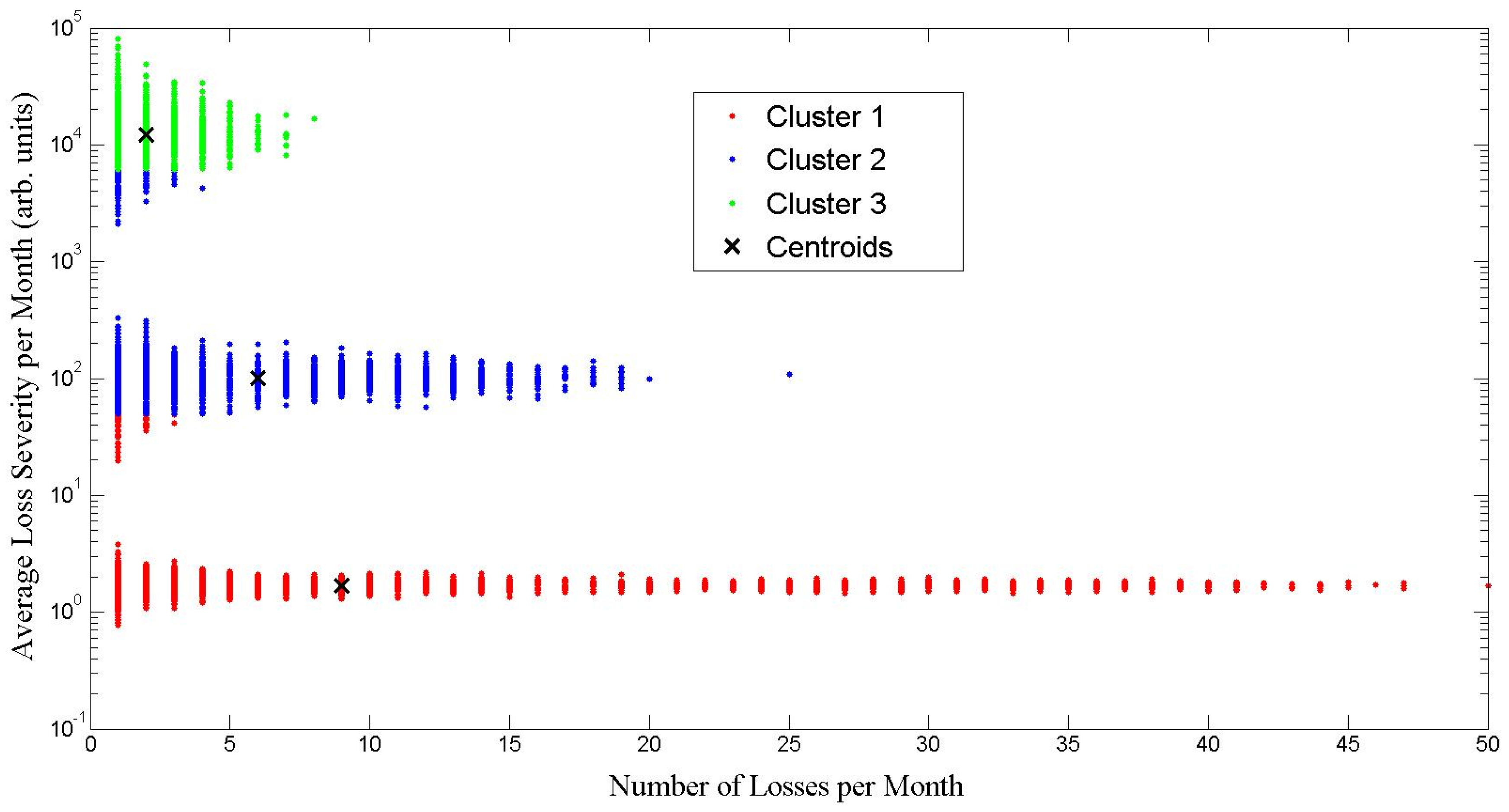
We describe results for two sample cases and show how the DPFS approach splits the loss frequency and loss severity data. The DPFS has two specific implementations, referred to as Method I and Method II, as described in Section 3. Figure 4 shows the results of DPFS Method I for the Scenario (I) simulated data. Note that the clustering algorithm finds three clusters (K = 3); namely, red, green and blue. The red points show the low loss severity region consisting of all types of loss frequencies; namely, high/medium/low. The green points represent the high loss severities which occur only in low frequency. The blue points symbolize the medium loss severity which occurs in low and medium frequencies. The clustering algorithm for Scenario (I) has a misclassification rate of less than 5%, as visually noted from the incorrect green and blue points in Clusters 1 and 2 in Figure 4. Through verification from a simulated dataset (where the results are known), we observe the merit of the clustering algorithm in finding the frequency/severity relationship into three categories: (1) low severity with all categories of frequency (high/medium/low); (2) medium severity with two categories of frequency (low/medium); (3) high severity, which only occurs with low frequency.
Figure 5 shows VaR estimation results for DPFS Method II applied to the simulated data: Scenario (II). This scenario consists of the separation of frequency and severity into three distinct regions: high frequency/low severity, medium frequency/medium severity, and low frequency/high severity. DPFS Method II correctly identifies three distinct frequency/severity regions with less than a 1% misclassification rate for the Scenario (II) simulated data. The clustering algorithm separates the data into three clusters of different severity levels. The upper right figure is a magnification of the high severity/low frequency region, while the lower left is the medium severity/medium frequency and the lower right corresponds to the low frequency/high severity case. Through this verification exercise using synthetic data from Scenario (II), the effectiveness of the DPFS Method II is demonstrated. We obtain similar results, as in Figure 4 and Figure 5, for all five simulated scenarios and five real-world datasets.

5.2. CPFS Performance

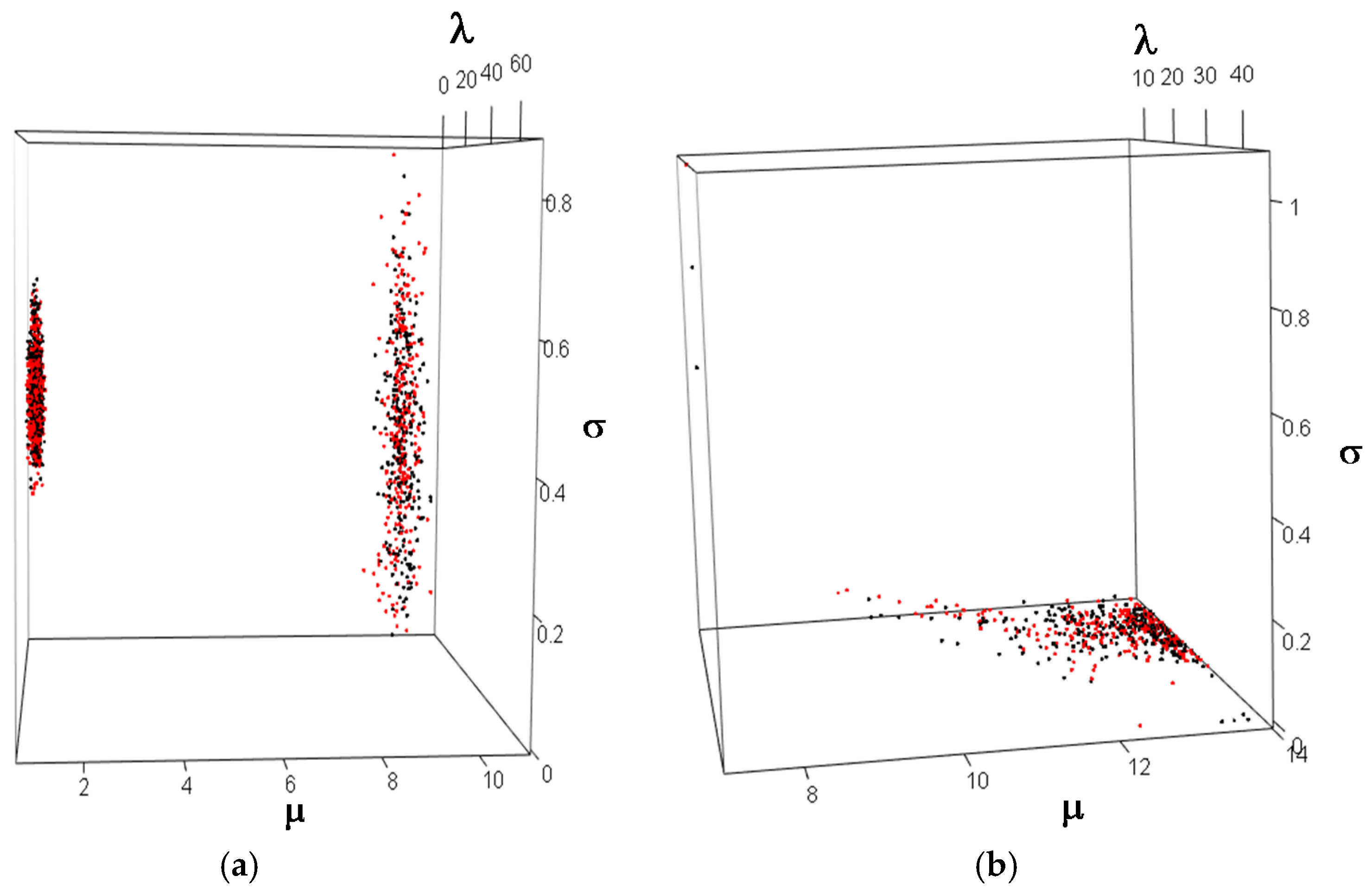
Two sample cases are given to show how the CPFS splits the frequency and severity loss data into three dimensions: the mean ( μ ) and the standard deviation ( σ ) of the severity parameters and the mean of the frequency parameter ( λ ). While the CPFS machinery can handle different types of copulas, we study the following cases: Gaussian, t, and Gaussian mixture. Figure 6a shows the performance of CPFS with a Gaussian mixture copula on Scenario (IV) (a clustered correlation between frequency and severity). Note that the Gaussian mixture copula surface (red points in the figure) fits the original simulated loss data (black points in the figure) closely. The performance of CPFS with the Gaussian copula on the chemical spills dataset is shown in Figure 6b. We observe that the Gaussian copula fits most of the data, including a few extreme points in the upper quadrant. We obtain similar figures, as in Figure 6a,b, for all five simulated scenarios and five real-world datasets.

5.3. VaR Estimation Comparisons between Classical, CPFS and DPFS Approaches

We compare the VaR estimation accuracy of the two new methodologies developed with the classical method on all simulated and real data sets. In order to benchmark the VaR estimation results, we use back-testing procedures. Since the simulation parameters are known a priori, we know the ground truth for the VaR estimate of the simulated data. For real datasets, we construct lower and upper 99% bootstrap confidence intervals for VaR using the original aggregated loss data (aggregate based on the frequency time unit of interest; i.e., monthly/annually) and use the bootstrap confidence intervals as the benchmark. Bootstrapping involves generating a large number (>10,000) of bootstrap datasets by sampling with replacement from the original loss data, then computing the sample VaR of each bootstrap dataset. The lower 0.5% and upper 99.5% percentiles are then taken as the lower and upper limits of the bootstrap 99% confidence interval. This approach follows the standard backtesting procedures which are used in VaR estimation (Campbell 2006).
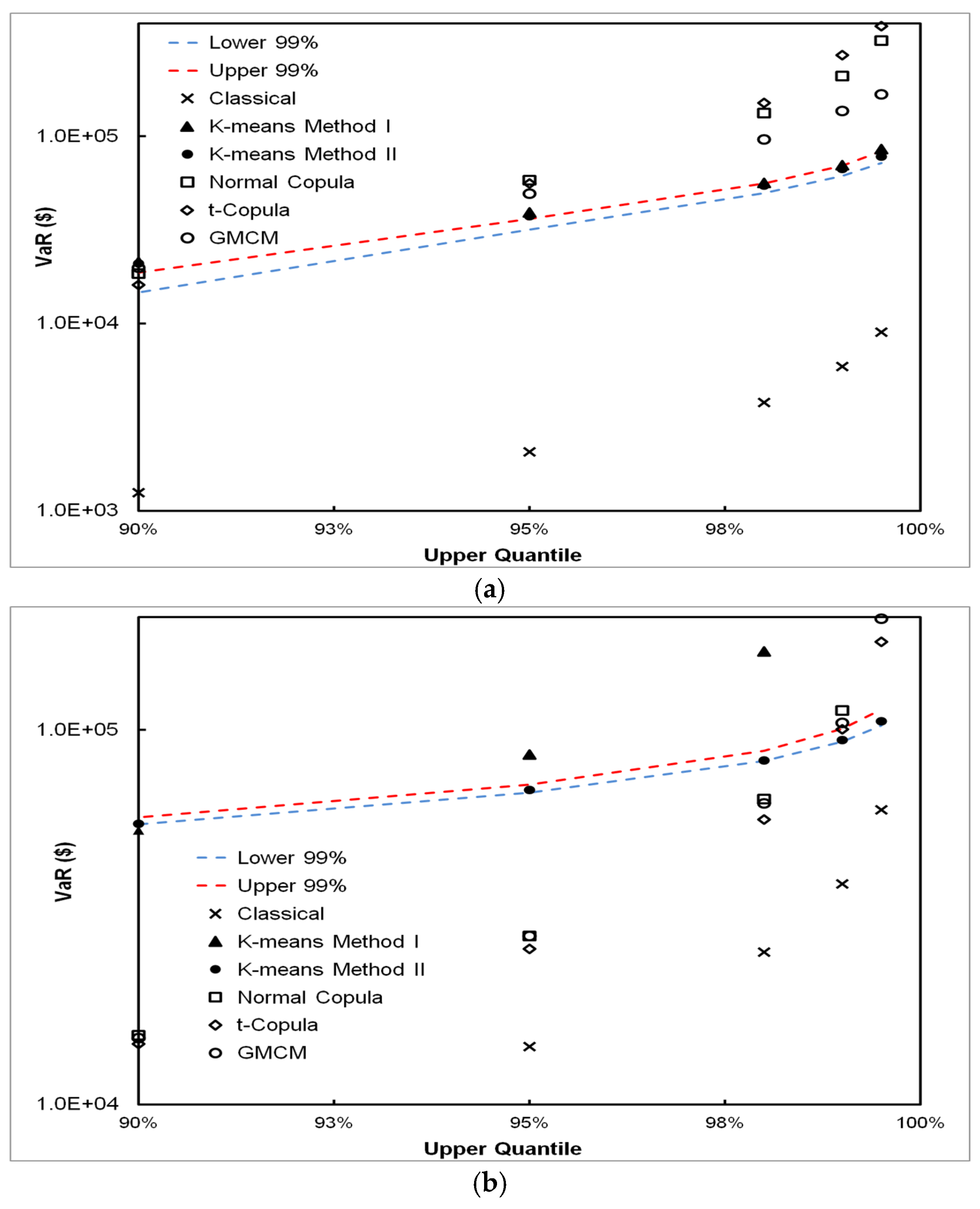
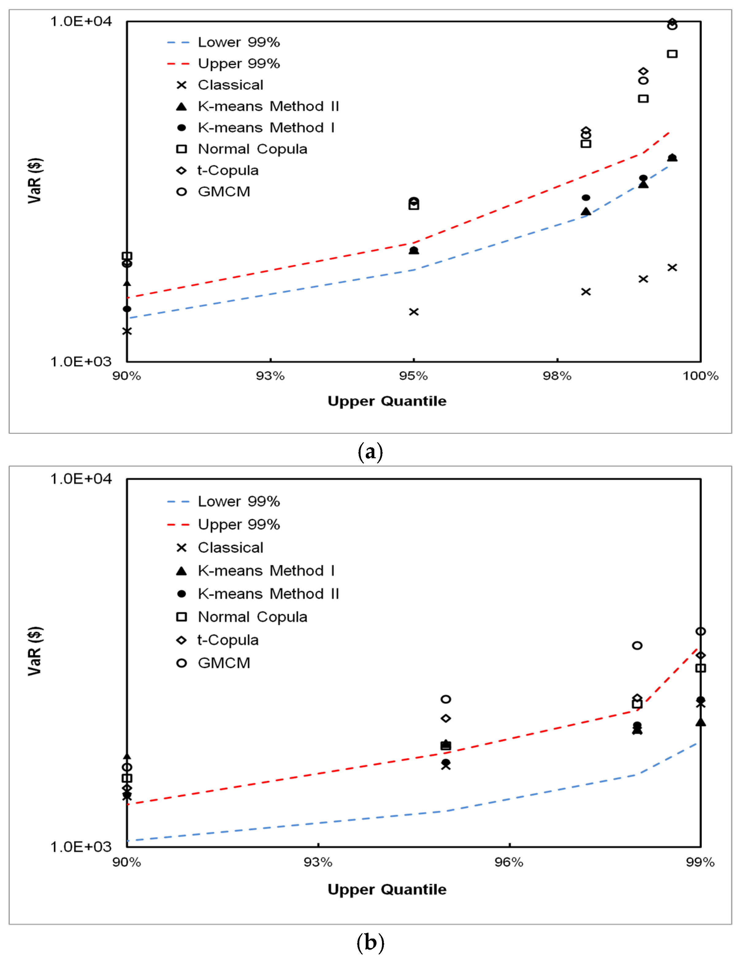
The upper panel in Figure 7 shows the 90%, 95%, 99%, 99.5%, and 99.9% VaR estimates for Scenario (I), together with the upper and lower bands of the 99% confidence intervals. For graphical analysis purposes, we show the confidence intervals for all cases, even though it is not needed for simulation data (where the true VaR is known a priori). The classical method underestimates VaR while DPFS VaR estimates fall within the interval for Scenario (I). The lower panel in Figure 7 shows the results obtained for Scenario (II). We observe that the DPFS Method II performs well, while the classical methodology grossly underestimates VaR and falls outside the confidence bands. For the extreme tails (99% and above), the t and Gaussian mixture copulas also fit the simulated data well.
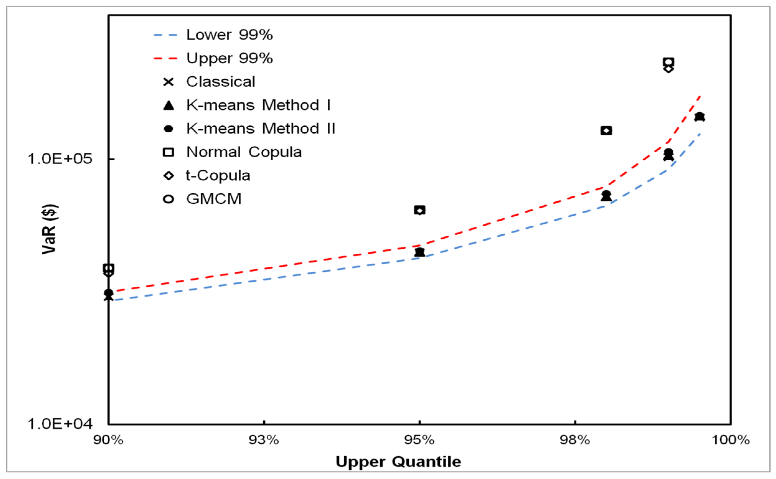
The results for Scenario (III) are presented in Figure 8; this is the scenario in which loss severity and loss frequency are independent. We observe that DPFS Method II and the classical method perform equally well. This shows that DPFS can handle loss data in which frequency and severity are independent, and that it is a viable alternative to the classical methodology.
Scenario (IV) and Scenario (V) results are presented in the upper and lower panels of Figure 9 respectively. Both the CPFS with Gaussian mixture copula in Scenario (IV) and t-copula in Scenario (V) performs well for 99% and higher VaR estimation, while all other methods either severely over-estimate or under-estimate the true VaR. In many risk management contexts, the 99% and higher VaR figures are of interest. Therefore, this shows that the CPFS method (with a Gaussian mixture copula) performs well for similar types of loss data situations. The DPFS K-means method does not perform well in Scenario (V) as there is a continuous linear relationship between loss frequency and loss severity, and one is therefore not able to model this relationship discretely, as required by the K-means algorithm.
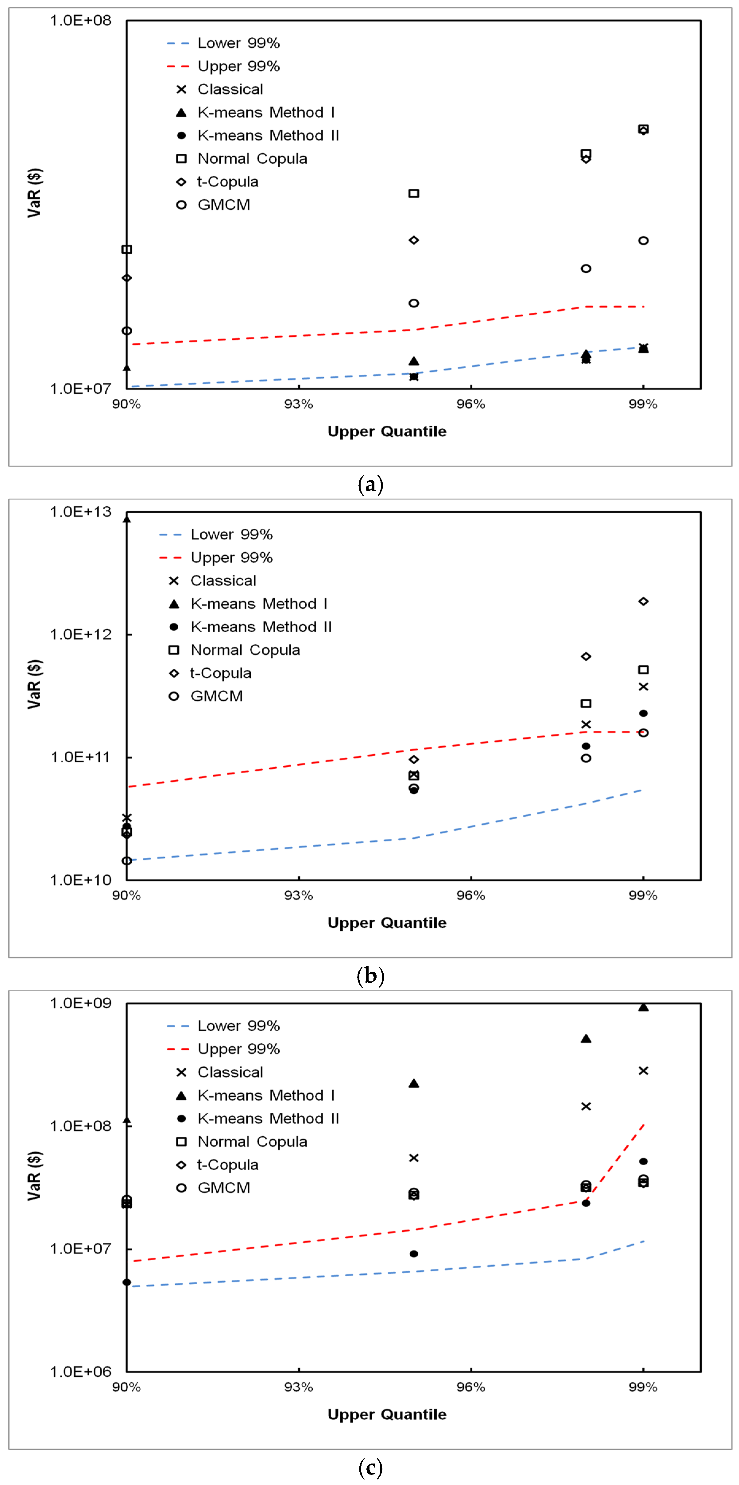
We present the validation results of these methodologies with real-world data, beginning with the data from the financial domain in Figure 10. The S & P 500 and DJIA results are presented in the upper and lower panels of Figure 10 respectively. For S & P 500, both DPFS Method I and Method II perform well in estimating VaR. The CPFS methods overestimate the VaR while the classical method severely underestimates the VaR. For the DJIA data, the DPFS Method II and the classical method perform well.
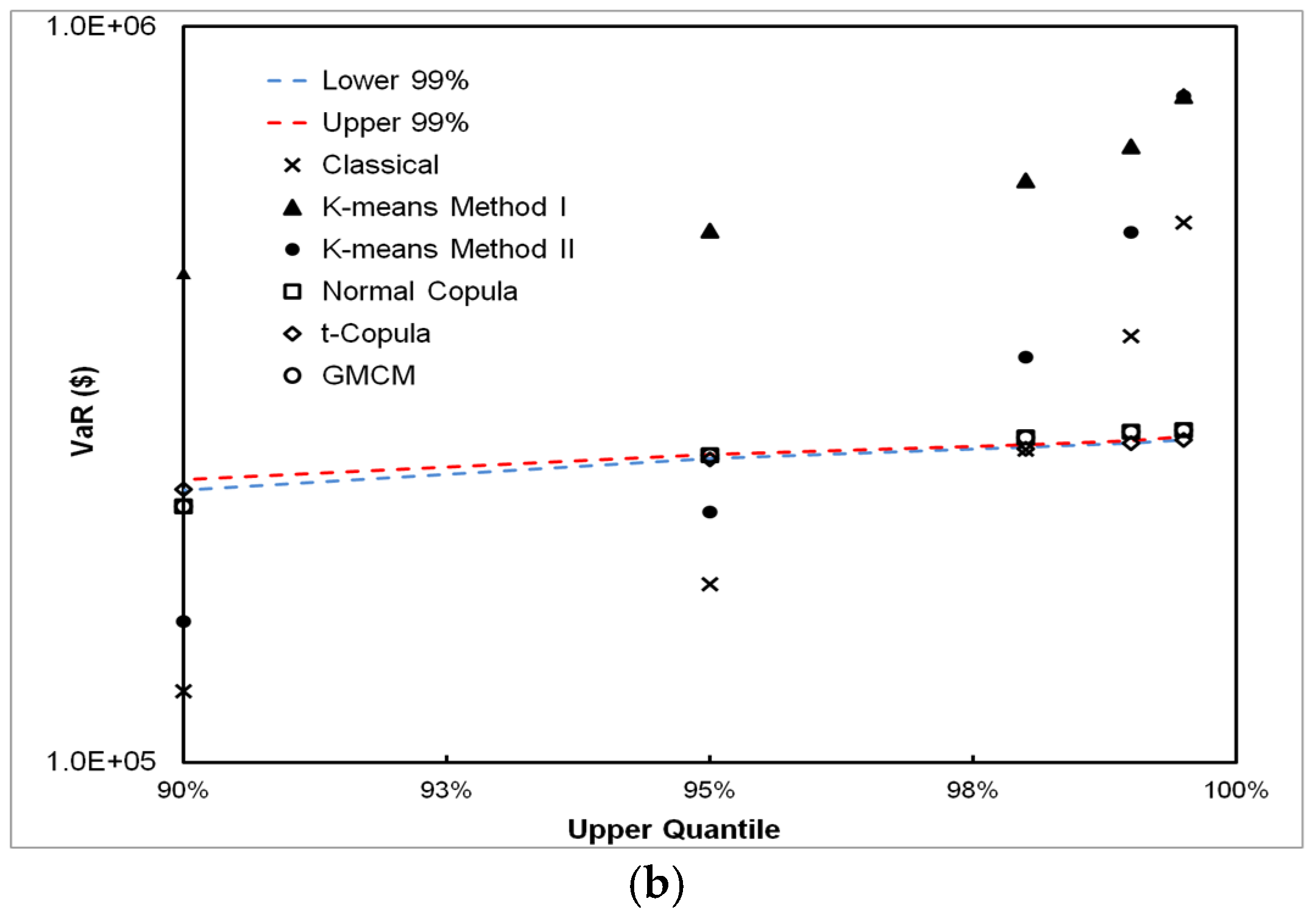
The results from the real-world datasets consisting of the non-financial domain are presented in Figure 11. The automobile accidents from the Australian VaR results are presented in the upper panel of Figure 11. The DPFS Method I performs the best in accurately estimating VaR. The classical method also provides reasonable estimates, and is only slightly outside (within 1%) the lower confidence band. The US hurricanes results are shown in the middle panel of Figure 11. The CPFS with a Gaussian mixture copula performs the best throughout the entire upper tail region. The classical method fails in the upper tail regions (98% and above). Finally, the chemical spills results are presented in the lower panel of Figure 11. The DPFS Method II performs well in all quantiles of VaR estimation, while for 99% and higher quantiles, CPFS estimates the VaR well (according to the bootstrap confidence bands). The classical methodology overestimates the VaR in this case by an order of magnitude. A strong correlation in the loss frequency and loss severity is observed in this dataset.
To summarize, the classical method performs poorly in 4 out of 5 of the simulated scenarios in which the independence assumption is violated. For the real datasets, the classical method fails to estimate the VaR within the 99% bootstrap confidence interval in 3 out of the 5 datasets. In comparison, the proposed new methodologies—DPFS or CPFS—provide accurate VaR estimates in instances when the classical method fails and also in instances where the classical method correctly estimates the VaR. This is observed in both simulated and real-world data.

6. Discussion

Scenarios (I) and (II) correspond to the discrete partitioning of the loss data based on severity and frequency. The DPFS method performs well for this type of data, as the DPFS adaptively clusters the data when there exist finite partitions between the loss frequency and the loss severity. For these two scenarios, the classical method grossly underestimates the VaR. In the risk-management context, underestimating the VaR exposes the institution to severe risks and even the potential of a catastrophic failure.
Scenario (III) satisfies the assumption of the independence between loss severity and loss frequency. The classical method robustly estimates VaR in this scenario. DPFS also matches the performance of the classical because it chooses not to partition the data (K = 0) when there exists independence of severity and frequency in the data.
Scenarios (IV) and (V) represent ideal cases for using the CPFS methodology in order to estimate VaR, as there is a high degree of continuous correlation between loss frequency and loss severity. Specifically, for Scenario (IV), the data comes from a mixture process, thus the Gaussian mixture copula provides the best VaR estimates. In Scenario (V), the synthetic data is generated with a perfect linear correlation between loss frequency and loss severity. The classical method fails to accurately estimate VaR in these two scenarios, as the independence assumption is violated. It is interesting to observe that the DPFS method did not work well in this context; this is because there is a continuous relationship between frequency and severity. In order to robustly estimate VaR in this situation, DPFS would need to generate a large number of clusters to mimic a continuous process from a discrete paradigm. This would result in a potential over-fitting of the data.
For the real-world data, we do not know a priori if the independence assumption holds true between loss severity and loss frequency. Looking at the non-financial domain, the chemical spills data bears similar distributional characteristics with the simulated Scenario (II), in that the loss frequency/severity relationship is discretely multi-modal. Therefore, DPFS performs well while the classical method overestimates the VaR. Our mathematical analysis in Section 3 confirms this empirical observation. Specifically, the overestimation is primarily due to the fact that the true aggregated loss process involves a scenario where the frequency component dominates the severity portion. The Australian automobile accident data, on the other hand, shows no relationship between loss frequency and loss severity, and thus the performance of the classical method along with DPFS works well for estimating VaR. Finally, the US hurricanes data also shows a multi-modal pattern for loss frequency and loss severity. CPFS, with a Gaussian mixture copula, performs well in estimating VaR, while the classical method performs poorly, due to the complex relationship found between loss severity and loss frequency.
The financial market loss data results provide some interesting insights. The difference between the DJIA and the S & P 500 results can be attributed to the fact that the losses during the US Great Depression of the 1920s and 1930s and the Second World War are included in the S & P 500 dataset. The DJIA data, on the other hand, started from the 1950s, when there was economic expansion in the US. Therefore, the S & P data had more instances of extreme loss events. Loss severity and loss frequency are known to be correlated in the case of extreme loss events, and the classical approach does not perform well. It is also interesting to note that the DJIA data did include small perturbations such as Black Monday 1987 and the 2007 credit crisis in the US. However, the markets recovered quickly (within days for 1987 and within a few years for 2007), and a prolonged effect on the overall VaR estimation might not have occurred. The Great Depression of the 1930s had a prolonged effect on US markets; this is also true of the start of the Second World War. This might have attributed to the major difference in the VaR estimation among these two similar loss data types. A summary chart of the overall performance across both simulated and real-world data is given in Table 1.
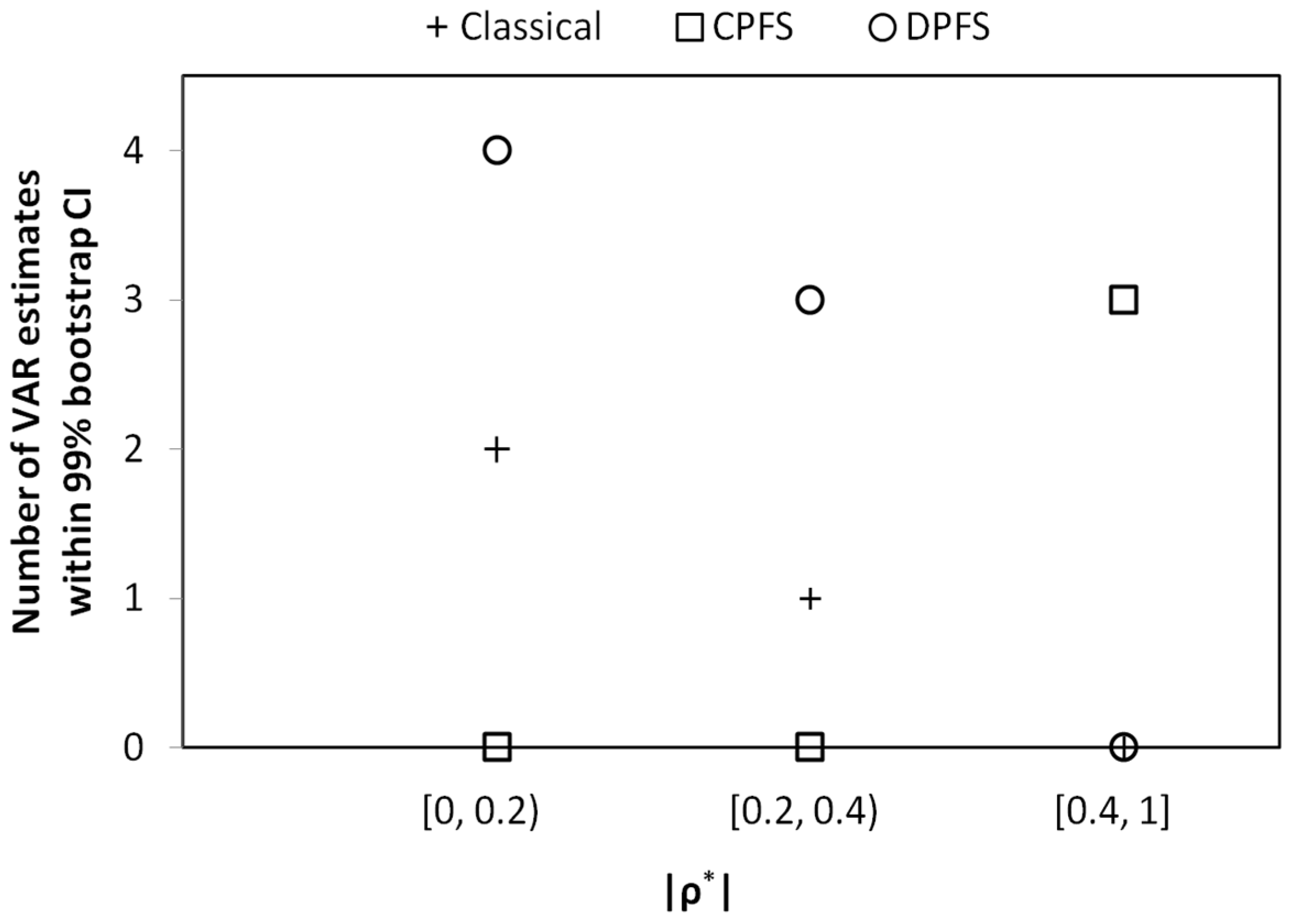
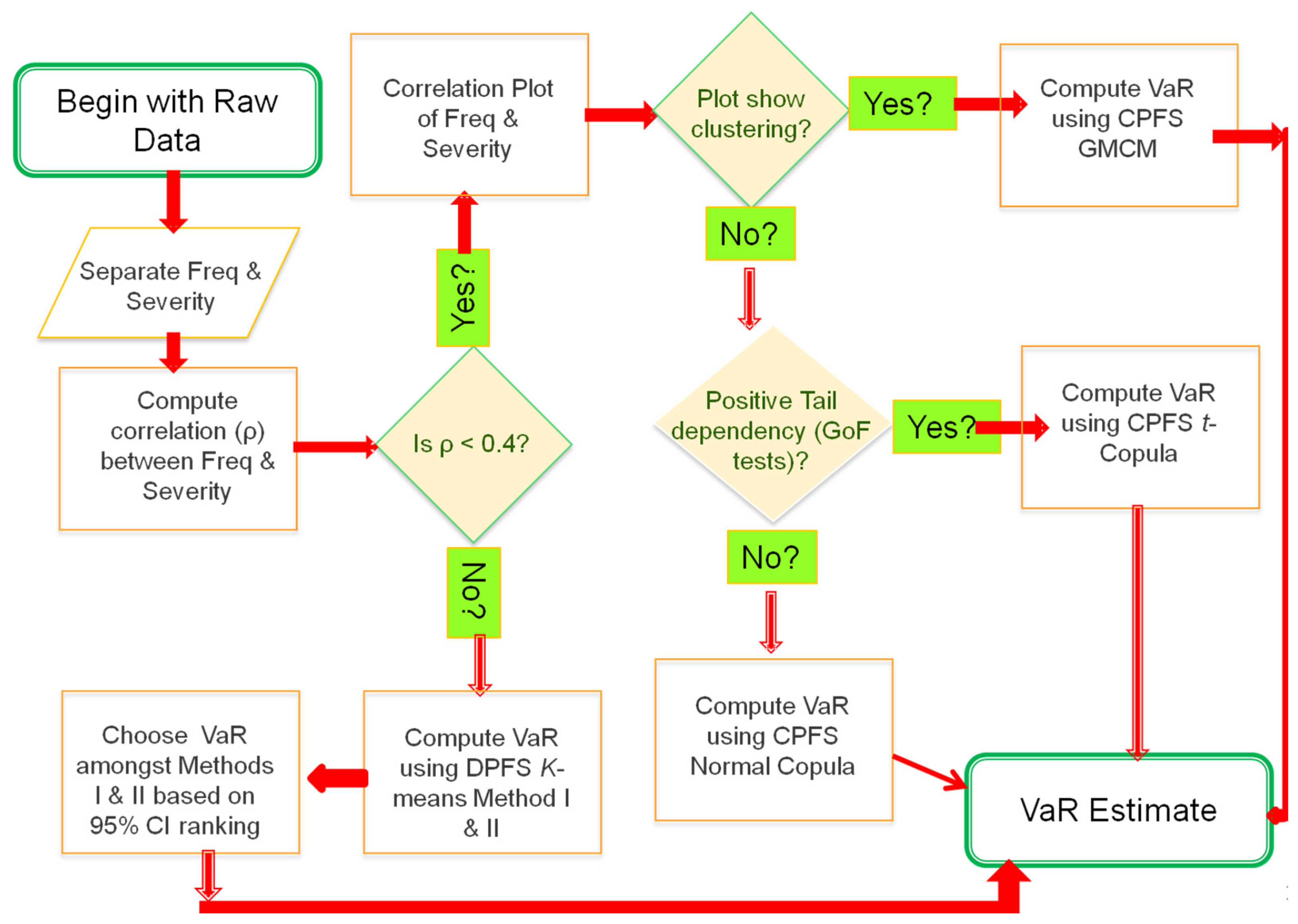
We note that both the DPFS and CPFS methodologies provide accurate VaR estimates in different loss data situations. To provide a practical guideline on how to choose the appropriate VaR method for a given data set, we plot the number of instances (where the VaR estimates are within the 99% historical bootstrap confidence intervals) versus the correlation values for the three methodologies of interest; namely, classical, CPFS and DPFS in Figure 12. It is interesting to note that, as the absolute magnitude of the correlation increases from zero, the accuracy of the classical methodology in estimating VaR goes down. The non-parametric DPFS methodology accurately estimates VaR consistently in the low/medium correlation range—namely, | ρ * | < 40%—while the CPFS method accurately estimates the VaR above 0.4. We thus observe a benchmark for using the CPFS methodology in VaR estimation when | ρ * | 40% and where ρ * is the correlation between loss severity and loss frequency as shown in Figure 12. Overall, we note that a single methodology does not universally estimate the VaR accurately in all instances of both simulated and real-world loss data. In Figure 13, we show a flowchart for selecting the appropriate method to robustly estimate VaR based on the loss data characteristics. To determine when to use the t-Copula from the Gaussian copulas, we note that the tail dependency between the loss severity and loss frequency needs to be tested. This is determined using statistical GoF tests. If the tail dependency is detected, then the t-copula should be used for the CPFS procedure instead of the Gaussian copula. This is because “t-copulas induce heavier joint tails than Gaussian copulas” (Cossin et al. 2010), as found in credit risk models.

7. Conclusions

This paper demonstrates the limitation of the classical approach in modern QRM for estimating Value-at-Risk. The classical approach underestimates the VaR in instances where there is a discrete partitioning of loss frequency and loss severity. In the cases in which a continuous correlation exists between loss frequency and loss severity, i.e., | ρ | 40%, the classical approach overestimates VaR. The classical approach estimates VaR accurately only in instances in which the independence assumption holds true. We implement two independent statistical methods; namely, the non-parametric DPFS method and the parametric CPFS method, which can more accurately estimate VaR for both independent and dependent relationships between loss frequency and loss severity. The strengths and weaknesses of DPFS and CPFS are investigated using both numerical simulation experiments and real-world data across multiple domains. No single method accurately estimates VaR within 99% bootstrap confidence bounds in different types of simulated and real-world data. We provide a procedure to guide practitioners in selecting the methodology for reliable VaR estimation for specific applications. We summarize the key findings below.
(i)
The classical approach works well if the independence assumption between frequency and severity approximately holds; however, it can grossly under or over-estimate VaR when this assumption does not hold. This is shown in both experiments on simulated and real-world data and through mathematical analysis, as described in the appendix.
(ii)
The DPFS method adapts to different frequency/severity relationships in which a finite partition can be found. In these situations, DPFS yields a robust VaR estimation.
(iii)
The CPFS method works best where a reasonable positive/negative correlation, e.g., | ρ | 0.4, between loss frequency and loss severity exists.
(iv)
We have found that, for all simulated and real-world datasets, either the CPFS or the DPFS methodology provides the best VaR estimate. We have not found a single case where either CPFS or DPFS performs worse than the classical method in estimating VaR. Therefore, even in instances of loss datasets where independence between loss frequency and loss severity is observed, the classical methodology is not necessarily needed for robust VaR estimation.
(v)
We provide a flowchart that can help risk practitioners in selecting the appropriate VaR estimation methodology.
To continue this work, one may explore the use of other unsupervised clustering techniques, such as the K-medoids (Chen and Hu 2006) and fuzzy clustering (Bose and Chen 2015; Byeon and Kwak 2015; Hirschinger et al. 2015) algorithms. Fuzzy clustering uses an artificial intelligence method for clustering data components instead of the standard distance metric as used by K-means and K-medoids. Optimization-based clustering can also be explored, using various validity indices to determine the quality of the clustering solution (Xu et al. 2010, 2012). Unlike the K-means approach, these methods are usually more computationally expensive. Mixture model-based clustering provides an alternative to the non-parametric clustering approaches in order to handle the complex relationships between loss severity and loss frequency (Xu and Wunsch 2009). However, computational challenges creep in for mixtures which combine a discrete Poisson distribution for frequency and a continuous lognormal distribution for severity. For example, a failure to converge to a global optimum can occur in numerical optimization. The study of trade-offs between the computational efficiency and the accuracy of the VaR estimation by different methodologies, e.g., classical, DPFS, CPFS, and the aforementioned mixture-based clustering can further advance our knowledge, and this topic can be addressed in the future.

Acknowledgments

This research has been partially supported by the National Science Foundation (NSF) and the Air Force Office of Scientific Research (AFOSR) under grant no. ECCS-1462409 and Army Research Office (ARO) under grant no. #W911NF-15-1-0409.

Author Contributions

This work comprises a portion of S.G.’s doctoral dissertation thesis. K.C.C. and J.X. served as S.G.’s doctoral dissertation advisors.

Conflicts of Interest

The authors declare no conflict of interest.

Appendix A. Proof of Proposition 1

From Section 3, recall that X ~ LN(μ, σ), Y ~ LN(μ/k, σ), M ~ Pois(λ) and N ~ Pois(λ/l). In Equations (3) and (4), we define two loss regimes: SX representing the “high severity/low frequency” regime and SY representing the “low severity/high frequency” regime, along with their mathematical definitions. Also, recall that in Case (I), we use a setup where mean severity dominates mean frequency, i.e., μ = O ( e λ ) . We also set 0 < σ < 1 and λ > 1 (i.e., greater than one event per time unit on average). For this calculation, we have also set μ to be large, i.e., μ >> 1. Case (I) thus represents a scenario with a small number of loss events of exponentially large severities (relative to the mean frequency). In Böcker and Klüppelberg (2005), it was shown that the VaR for the aggregated loss over a time period of length T = 1 with a severity distributed as LN( μ , σ) and a frequency modeled by Pois( λ ) can be approximated in closed-form as the quantile κ → 1:
VaR ( κ ) = exp { μ σ Φ 1 ( 1 κ λ ) }
Using Equation (A1), we have the VaR for SX and SY as shown below:
VaR ( S X   |   κ , μ , σ , λ l ) exp [ μ σ Φ 1 ( 1 κ λ / l ) ]
VaR ( S Y   |   κ , μ k , σ , λ ) exp [ μ k σ Φ 1 ( 1 κ λ ) ]
Substituting μ = e λ in the right hand side of Equations (A2) and (A3), we have
VaR ( S X   |   κ , μ , σ , λ l ) exp [ e λ σ Φ 1 ( 1 κ λ / l ) ]
VaR ( S Y   |   κ , μ k , σ , λ ) exp [ e λ k σ Φ 1 ( 1 κ λ ) ]
Next, we use the probit approximation for the inverse normal CDF, which is related to the inverse error function (Giles 2011) as the following:
Φ 1 ( A 2 ( x + 1 ) ) = 2 erf 1 ( Ax )
where A is a constant. The Maclaurin series expansion of erf−1(y) has the following property (Giles 2011):
erf 1 ( y ) y + O ( y 3 )
Next with A = (1−κ), and y = 1/λ, the following is obtained:
Φ 1 ( A λ ) erf 1 ( 2 A λ 1 ) erf 1 ( 2 A λ 1 ) 2 A λ 1 + O [ ( 2 A λ 1 ) ] 3
Since λ > 1, and κ → 1, the higher order terms can be ignored. Therefore, the right-hand side of Equations (A4) and (A5) can be approximated as the following:
VaR ( S X   |   κ , μ , σ , λ l ) exp [ e λ σ 2 l ( 1 κ ) λ A 1 ]
VaR ( S Y   |   κ , μ k , σ , λ ) exp [ e λ k σ ( 2 2 κ λ ) 1 B ]
Next, examining the rate of change of A’ and B’ (from Equations (A7) and (A8) above) with respect to λ:
A λ = e λ + σ 2 l ( 1 κ ) λ 2
B λ = e λ k + σ 2 ( 1 κ ) λ 2
Now, observing the region of the extreme right tail, i.e., κ 1 , lim κ 1 σ 2 l ( 1 κ ) λ = 0 for λ > 1 and l fixed and finite. Likewise, lim κ 1 σ 2 ( 1 κ ) λ = 0 for λ > 1 is obtained. So, the rate of change of A is larger than B with respect to λ because k > 1. In addition, the dominant term in both A and B is their first term, therefore VaR(SX | κ) > VaR(SY | κ) as κ 1 .
In Case (II), frequency dominates severity. We use the mean-adjusted VaR approximation formula from (Böcker and Sprittulla 2006) for a LN(μ, σ) severity and Pois(λ) frequency as the following:
VaR ( κ ) = exp { μ σ Φ 1 ( 1 κ λ ) } + ( λ 1 ) exp [ μ + σ 2 2 ]
The above formula translates into the following cases:
VaR ( S X   |   κ , μ , σ , λ l ) exp [ μ σ Φ 1 ( 1 κ λ l ) ] + { λ l 1 } exp ( μ ) exp ( σ 2 2 )
VaR ( S Y   |   κ , μ k , σ , λ ) exp [ μ k σ Φ 1 ( 1 κ λ ) ] + { λ 1 } exp ( μ k ) exp ( σ 2 2 )
For Case (II), λ = e e μ is substituted for λ in the RHS of Equations (A10) and (A11). In addition, the approximation of Φ 1 ( · ) (as in the above Case (I)) is also used next as the following:
VaR ( S X   |   κ , μ , σ , λ l ) exp [ μ σ 2 l ( 1 κ ) exp ( e μ ) 1 ] + { exp ( e μ ) l 1 } exp ( μ ) exp ( σ 2 2 )
VaR ( S Y   |   κ , μ k , σ , λ ) exp [ μ k σ 2 ( 1 κ ) exp ( e μ ) 1 ] + { exp ( e μ ) 1 } exp ( μ k ) exp ( σ 2 2 )
Since exp ( e μ ) >> exp ( μ ) , the right-hand side of Equation (A13) is larger than the right-hand side of Equation (A12) (since l > 1). That implies VaR( S Y   |   κ ) > VaR( S X   |   κ ) . Thus, it has been shown that for Case (I) the true VaR, i.e., VaR κ ( * ) , for VaR( S Z | κ) is approximated as the following:
lim κ 1 VaR ( S Z   |   κ ) VaR ( S X   |   κ , μ , σ , λ l ) exp [ μ σ Φ 1 ( 1 κ λ l ) ]
Likewise, for Case (II) the true VaR, i.e., VaR κ ( * ) , for VaR( S Z | κ) is approximated as the following:
lim κ 1 VaR ( S Z   |   κ ) VaR ( S Y   |   κ , μ k , σ , λ ) exp [ μ k σ Φ 1 ( 1 κ λ ) ]
We now consider how to calculate VaR κ ( C ) and the VaR κ ( * ) for both Cases (I) and (II). To begin, the classical approach for the frequency component of S Z is calculated as the following:
E[N] + E[M] = λ + λ/l = (l + 1)λ/l
For the severity component, since Z = p*X + (1 − p)*Y, where p = 1/(l + 1), (as defined in Equation (5)), we have
E[Z] = (1 − p)*E[Y] + p*E[X]; Var[Z] = p2*Var[X] + (1 − p)2*Var[Y].
By Fenton–Wilkinson approximation, the central moment matching (Mehta et al. 2007) is used to estimate a single log-normal distribution for Z as the following:
E [ Z ] = exp { μ Z + 0 . 5 * σ Z 2 } , Var [ Z ] = ( exp { σ Z 2 } 1 * exp ( 2 μ Z + σ Z 2 ) .
We next follow the Fenton–Wilkinson approach and perform the moment matching as follows:
exp { μ Z + 0 . 5 * σ Z 2 } = ( 1 p ) exp { 2 μ + k σ 2 2 k } + p exp { 2 μ + σ 2 2 } , exp { μ Z + 0 . 5 * σ Z 2 } = exp { 2 μ + σ 2 2 } { p + ( 1 p ) exp [ μ k μ ] } , μ Z = 2 μ + σ 2 2 + log { p + ( 1 p ) exp [ μ k μ ] } 0.5 σ Z 2
For variances, we use the Fenton–Wilkinson approach and perform moment matching as following:
( exp { σ Z 2 } 1 ) exp ( 2 μ Z + σ Z 2 ) = p 2 [ exp { σ 2 } exp { 2 μ + σ 2 } exp { 2 μ + σ 2 } Var [ X ] ] + ( 1 p ) 2 [ exp { σ 2 } exp { 2 μ k + σ 2 } exp { 2 μ k + σ 2 } Var [ Y ] ] LHS = ( 1 l + 1 ) 2 [ exp { σ 2 + μ } ] [ exp { σ 2 + μ } exp { μ } + l 2 exp { 2 μ k μ + σ 2 } l 2 exp { 2 μ k μ } γ ]
Taking a logarithm on both sides yields the following:
2 μ Z + σ Z 2 + log { exp [ σ Z 2 ] 1 } = log ( p 2 ) + [ σ 2 + μ ] + log ( γ )
By substituting the RHS of Equation (A16) for μ Z into the LHS of Equation (A17), we obtain the following:
2 μ + σ 2 + 2 log { p + ( 1 p ) exp [ μ k μ ] ϱ } + log { exp [ σ Z 2 ] 1 } = log ( p 2 ) + [ σ 2 + μ ] + log ( γ ) log { exp [ σ Z 2 ] 1 } = μ log ( ϱ 2 ) + log ( γ ) + log ( p 2 ) log { exp [ σ Z 2 ] 1 } = log ( γ exp { μ } exp ( C ) ϱ 2 ) ,   where C = log ( p 2 ) σ Z 2 = log [ γ exp { μ } exp ( C ) ϱ 2 + 1 ]
where
γ = [ exp { σ 2 + μ } exp { μ } + l 2 exp { 2 μ k μ + σ 2 } l 2 exp { 2 μ k μ } ] ,   ϱ = { p + ( 1 p ) exp [ μ k μ ] } .
The above simplification leads to the following:
μ z = μ + σ 2 2 + log { p + ( 1 p ) exp [ μ k μ ] } 0.5 log [ γ exp { μ } exp ( C ) ϱ 2 + 1 ]
For the classical estimate of VaR, the single loss VaR approximation formula from Böcker and Klüppelberg (2005) is used below:
VaR ( S Z C   |   κ μ z , σ Z , ( l + 1 ) λ l ) exp [ μ z σ Z Φ 1 ( ( 1 κ ) ( l + 1 ) λ l ) ]
where μ z is calculated in Equation (A19) and σ Z 2 is calculated in Equation (A18). With the classical VaR estimation, we are now ready to compare this with both Case (I) and Case (II). For Case (I), we perform an analysis with μ >> 1 and as κ → 1 for μ z and σ Z 2 next:
log [ γ exp { μ } exp ( C ) ϱ 2 + 1 ] = log [ ( l 2 exp { σ 2 + 2 μ [ 1 k 1 ] } + [ exp { σ 2 } l 2 exp { 2 μ [ 1 k 1 ] } ) exp ( C ) { p + ( 1 p ) exp [ μ k μ ] } 2 + 1 ] LHS = log [ exp ( C ) l 2 exp { σ 2 + 2 μ [ 1 k 1 ] } + exp ( C ) [ exp { σ 2 } l 2 exp { 2 μ [ 1 k 1 ] } { p + ( 1 p ) exp [ μ k μ ] } 2 + 1 ]
Since σ is finite and fixed while μ is large, the RHS of the above equation can be approximated by:
log [ exp ( C ) γ exp { μ } ϱ 2 + 1 ] log [ { exp { σ 2 } 1 } x + 1 ]
With the Taylor approximations for log(1 + x) and exp{x},
log ( 1 + x ) = x O ( x 2 ) for   | x |   < 1
σ Z 2 = log [ exp ( C ) γ exp { μ } ϱ 2 + 1 ] log [ { exp { σ 2 } 1 } x + 1 ] exp { σ 2 } 1 σ 2
log { p [ 1 + [ 1 p 1 ] exp [ μ ( 1 k 1 ) ] ] } log [ 1 + [ 1 p 1 ] exp [ μ ( 1 k 1 ) ] ]
exp [ μ ( 1 k 1 ) ] 1 + μ ( 1 k 1 )
Substituting the above approximations of Equation (A21) and Equation (A20) into Equation (A18), we have
μ Z 1 + μ k ,   σ Z 2 σ 2 exp [ μ Z σ Z Φ 1 ( ( 1 κ ) ( l + 1 ) λ l ) ] Classical exp [ μ k + 1 σ Φ 1 ( l ( 1 κ ) ( l + 1 ) λ ) ]
In this scenario, since μ >> λ, by taking the limit when the upper quantile approaches 1, i.e., κ→1, Φ 1 ( · ) decreases approximately O [ 1 exp { x 2 } ] , thus μ k + 1 σ Φ 1 ( ( 1 κ ) ( l + 1 ) λ l ) μ σ Φ 1 ( 1 κ λ l )
exp [ μ k + 1 σ Φ 1 ( ( 1 κ ) ( l + 1 ) λ l ) ] exp [ μ σ Φ 1 ( 1 κ λ l ) ]
To see why the Φ 1 ( · ) component is negligible, one can differentiate the inverse normal CDF to understand its rate of change:
δ δ x [ Φ 1 ( x ) ] = 1 ϕ ( Φ 1 ( x ) ) ,
where ϕ is the standard normal pdf. So the rate of increase of [ μ k + 1 σ Φ 1 ( ( 1 κ ) ( l + 1 ) λ l ) ] is determined by μ k versus that of [ μ σ Φ 1 ( ( 1 κ ) λ 2 ) ] is determined by μ, i.e., the first term only.
Therefore, the VaR obtained from classical approach, VaR κ ( C ) , is smaller than the true VaR ( VaR κ ( * ) ), under the specifications present in Case (I). The procedure for a comparison between the classical approach and the true VaR for Case (II) is shown next. Using the mean-adjusted VaR approximation formula in (Böcker and Sprittulla 2006), the adjusted VaR analysis is implemented from Equation(A10) for a general aggregated loss SQ as the following:
VaR ( S Q Mean   |   κ , μ , σ , λ ) exp [ μ σ Φ 1 ( 1 κ λ ) ] + ( λ 1 ) exp [ μ + σ 2 2 ]
We apply the above formula for S Z next:
exp [ μ z σ z Φ 1 ( 1 κ ( l + 1 ) λ l ) ] + ( ( l + 1 ) λ l 1 ) exp { μ z + σ z 2 2 } Classical exp [ μ k + 1 σ Φ 1 ( l ( l κ ) ( l + 1 ) λ ) ] + ( ( l + 1 ) λ l 1 ) exp [ 1 + 2 μ + κ σ 2 2 κ ]
It can be shown that the true VaR, i.e., VaR κ ( * ) corresponds to VaR( S Z | κ) is approximately (from Equation (A15)):
lim κ 1 VaR ( S Z   |   κ ) VaR ( S Y   |   κ , μ k , σ , λ ) VaR ( S Y   |   κ , μ k , σ , λ ) exp [ μ k σ Φ 1 ( 1 κ λ ) ] + ( λ 1 ) exp ( μ k + σ 2 2 )
Note that the inverse normal CDF, Φ 1 ( · ) decreases approximately O [ 1 exp { x 2 } ] , and therefore exp [ μ k + 1 σ Φ 1 ( l ( 1 κ ) ( l + 1 ) λ ) ] exp [ μ k σ Φ 1 ( 1 κ λ ) ] , for small μ (as in the situation in Case (II)).
However, since λ >> μ, ( ( l + 1 ) λ l 1 ) exp [ 1 + 2 μ + k σ 2 2 k ] ( λ 1 ) exp ( μ + σ 2 2 ) . Therefore,
exp [ μ k + 1 σ Φ 1 ( l ( 1 κ ) ( l + 1 ) λ ) ] + ( ( l + 1 ) λ l 1 ) exp [ 1 + 2 μ + k σ 2 2 k ] exp [ μ k σ Φ 1 ( 1 κ λ ) ] + ( λ 1 ) exp ( μ + σ 2 2 )
Therefore, the classical VaR estimate, VaR κ ( C ) , is larger, under the specified conditions in Case (II), than VaR κ ( * ) . ■

Appendix B. Description of the Process for Generating Simulated Scenarios (I)–(V)

From Section 4.1, recall that we simulate data for verification purposes of classical, CPFS and DPFS methodologies. For all scenarios, the loss severity is generated from a LN(μ, σ) distribution while the loss frequency is generated from a Pois(λ) distribution. Scenario (I) partitions the frequency and severity into high/medium/low regions with a one-to-many relationship between frequency and severity, as shown in Figure 2. The low severity region is generated from LN(0.5, 0.25), while the medium severity is generated from LN(4.5, 0.5), and the high severity is generated from a LN(9.3, 0.6) distribution. The low frequency is generated from a Pois(2) distribution while the medium frequency is generated from a Pois(10) distribution; the high frequency is generated from a Pois(30) distribution. Algorithm A1 provides the details for generating simulated Scenario (I) data for simulation size n.
Algorithm A1 Procedure for generating synthetic data corresponding to Scenario (I)
1. For i = 1 to n months/years do
 (a) Generate a uniform random number, u ~ U[0, 1].
  (I) If (u ≤ 1/2) then
   (I.1) Generate a random realization of λLow ~ Pois(2)
   (I.2) Generate discrete uniform (DU) random number m {1,2,3}
   (I.3) If (m = 1) then
    Generate losses X 1 , X 2 , , X λ L o w ~ LN(0.5, 0.25)
    Elseif (m = 2) then
    Generate losses X 1 , X 2 , , X λ L o w ~ LN(4.5, 0.5)
    Else
    Generate losses X 1 , X 2 , , X λ L o w ~ LN(9.3, 0.6)
    End if
  (II) If (1/2 < u ≤ 5/6) then
   (II.1) Generate a random realization of λMedium ~ Pois(10)
   (II.2) Generate discrete uniform random number m {1,2}
   (II.3) If (m = 1) then
    Generate losses X 1 , X 2 , , X λ M e d i u m ~ LN(0.5, 0.25)
    Else
    Generate losses X 1 , X 2 , , X λ M e d i u m ~ LN(4.5, 0.5)
    End if
  (III) Else
   (III.1) Generate a random realization of λHigh ~ Pois(30)
   (III.2) Generate losses X 1 , X 2 , , X λ H i g h ~ LN(9.3, 0.6)
    End if
 (b) Return loss frequency (λLow/λMedium/λHigh)
 (c) Return loss severities for month/year i
2. End for loop
Scenario (II) partitions the frequency and severity into high/medium/low regions with a one-to-one relationship between frequency and severity, as shown in Figure 2. The low/medium/high severity and frequency parameters are identical to that in Scenario (I). Algorithm A2 provides the details for generating simulated Scenario (II) data for simulation size n.
Algorithm A2 Procedure for generating synthetic data corresponding to Scenario (II)
1. For i = 1 to n months/years do
 (a) Generate a random realization of λLow ~ Pois(2)
  (I) Generate losses X 1 , X 2 , , X λ L o w ~ LN(9.3, 0.6)
 (b) Generate a random realization of λMedium ~ Pois(10)
  (I) Generate losses X 1 , X 2 , , X λ M e d i u m ~ LN(4.5, 0.5)
 (c) Generate a random realization of λHigh ~ Pois(30)
  (I) Generate losses X 1 , X 2 , , X λ H i g h ~ LN(0.5, 0.25)
 (d) Compute frequency for month/year i = λLow + λMedium + λHigh
 (e) Return loss frequency (λLow + λMedium + λHigh)
 (f) Return loss severities for month/year i
2. End for loop
Scenario (III) generates data where the loss frequency and loss severity are independent. The loss severity is generated from LN(5, 2), while the frequency is generated from Pois(14) independently. Algorithm A3 provides the details for generating simulated Scenario (III) data for simulation size n.
Algorithm A3 Procedure for generating synthetic data corresponding to Scenario (III)
1. For i = 1 to n months/years do
 (a) Generate a random realization of λunique ~ Pois(14)
  (I) Generate losses X 1 , X 2 , , X λ u n i q u e ~ LN(5, 2)
 (b)Return loss frequency (λunique)
 (c) Return loss severities for month/year i
2. End for loop
Scenario (IV) corresponds to the simplex mixture-regime problem that we introduced in Section 3.1. We are generating data from low frequency/high severity as region 1 and high frequency/low severity as region 2. Algorithm A4 provides the details for generating simulated Scenario (IV) for simulation size n.
Algorithm A4 Procedure for generating synthetic data corresponding to Scenario (IV)
1. For i = 1 to n months/years do
 (a) Generate a uniform random number, u ~ U [0, 1].
  (I) If (u ≤ 3/10) then
    (I.1) Generate a random realization of λLow ~ Pois(5)
    (I.2) Generate losses X 1 , X 2 , , X λ L o w ~ LN(10, 0.5)
   Else
    (I.3) Generate a random realization of λLow ~ Pois(5)
    (I.4) Generate losses X 1 , X 2 , , X λ H i g h ~ LN(1, 0.5)
   End if
 (b) Return loss frequency (λLow/λHigh)
   (c) Return loss severities for month/year i
2. End for loop
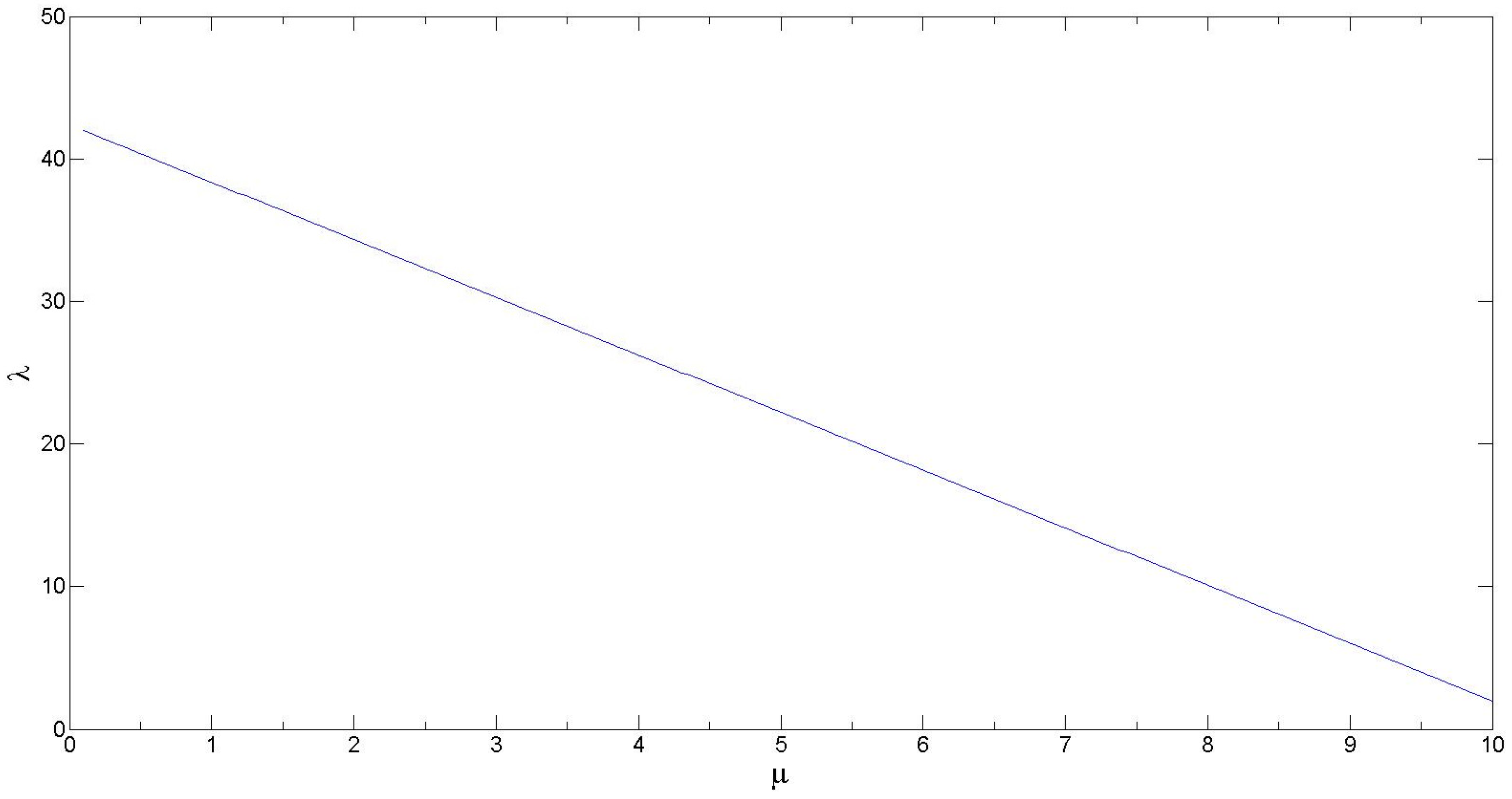
Scenario (V) corresponds to the case with perfect linear relationship between frequency and severity as previously shown in Figure 3. We show the exact relationship between λ and μ in Figure A1. Algorithm A5 provides the details for generating simulated Scenario (V) data for simulation size n.
Figure A1. Plot showing the linear relationship between average loss frequency (λ) and average loss severity (μ). This line can be generated using the following equation: λ = 20 . 20 ¯ μ + 212 . 02 ¯ .
Risks 05 00041 g014
Algorithm A5 Procedure for generating synthetic data corresponding to Scenario (V)
1. For i = 1 to n months/years do
 (a) Generate a discrete uniform random number, λFixed ~ DU[10, 210].
 (b) Given a λFixed, calculate the corresponding μi from the Figure A1.
 (c) Generate losses X 1 , X 2 , , X λ F i x e d ~ LN(μi, 0.1)
 (d) Return loss frequency (λFixed) for month/year i
 (e) Return loss severities for month/year i
2. End for loop
With the above Algorithms (A1)–(A5), we generate simulated Scenarios (I)–(V) for simulation size n of 1,000,000.

References

  1. OpRisk Advisory, and Towers Perrin. 2010. A New Approach for Managing Operational Risk: Addressing the Issues Underlying the 2008 Global Financial Crisis. Sponsored by Joint Risk Management, Section Society of Actuaries, Canadian Institute of Actuaries & Casualty Actuarial Society. Available online: https://www.soa.org/research-reports/2009/research-new-approach/ (accessed on 25 July 2017).
  2. Andersson, Frederick, Helmut Mausser, Dan Rosen, and Stanislav Uryasev. 2001. Credit risk optimization with conditional value-at-risk criterion. Mathematical Programming 89: 273–91. [Google Scholar] [CrossRef]
  3. Aue, Falko, and Michael Kalkbrener. 2006. LDA at work: Deutsche Bank’s approach to quantifying operational risk. Journal of Operational Risk 1: 49–93. [Google Scholar] [CrossRef]
  4. Balthazar, Laurent. 2006. From Basel 1 to Basel 3. In From Basel 1 to Basel 3: The Integration of State-of-the-Art Risk Modeling in Banking Regulation. London: Palgrave Macmillan, pp. 209–13. [Google Scholar]
  5. Bayestehtashk, Alireza, and Izhak Shafran. 2015. Efficient and accurate multivariate class conditional densities using copula. Paper presented at the 2015 IEEE International Conference on Acoustics, Speech and Signal Processing (ICASSP), Brisbane, QLD, Australia, April 19–24. [Google Scholar]
  6. Bilgrau, Anders E., Poul S. Eriksen, Jakob G. Rasmussen, Hans E. Johnsen, Karen Dybkær, and Martin Bøgsted. 2016. GMCM: Unsupervised clustering and meta-analysis using Gaussian mixture copula models. Journal of Statistical Software 70: 1–23. [Google Scholar] [CrossRef]
  7. Böcker, Klaus, and Claudia Klüppelberg. 2005. Operational VaR: A closed-form approximation. Risk-London-Risk Magazine Limited 18: 90. [Google Scholar]
  8. Böcker, Klaus, and Jacob Sprittulla. 2006. Operational VAR: Meaningful means. Risk 19: 96–98. [Google Scholar]
  9. Bose, Indranil, and Xi Chen. 2015. Detecting the migration of mobile service customers using fuzzy clustering. Information & Management 52: 227–38. [Google Scholar]
  10. Byeon, Yeong-Hyeon, and Kuen-Chang Kwak. 2015. Knowledge discovery and modeling based on Conditional Fuzzy Clustering with Interval Type-2 fuzzy. Paper presented at the 2015 7th International Joint Conference on Knowledge Discovery, Knowledge Engineering and Knowledge Management (IC3K), Lisbon, Portugal, 12–14 November; vol. 1, pp. 440–44. [Google Scholar]
  11. Campbell, Sean D. 2006. A review of backtesting and backtesting procedures. The Journal of Risk 9: 1. [Google Scholar] [CrossRef]
  12. Charpentier, Arthur, ed. 2014. Computational Actuarial Science with R. Boca Raton: CRC Press. [Google Scholar]
  13. Chavez-Demoulin, Valérie, Paul Embrechts, and Marius Hofert. 2016. An extreme value approach for modeling operational risk losses depending on covariates. Journal of Risk and Insurance 83: 735–76. [Google Scholar] [CrossRef]
  14. Chen, Yen-Liang, and Hui-Ling Hu. 2006. An overlapping cluster algorithm to provide non-exhaustive clustering. European Journal of Operational Research 173: 762–80. [Google Scholar]
  15. Cossin, Didier, Henry Schellhorn, Nan Song, and Satjaporn Tungsong. 2010. A Theoretical Argument Why the t-Copula Explains Credit Risk Contagion Better than the Gaussian Copula. Advances in Decision Sciences 2010: 1–29, Article ID 546547. [Google Scholar] [CrossRef]
  16. Data available at National Response Center. Available online: http://nrc.uscg.mil/ (accessed on 1 January 2016).
  17. Data available from Yahoo Finance. 2017. Available online: https://finance.yahoo.com/quote/%5EDJI/history?p=%5EDJI(DJIA); https://finance.yahoo.com/quote/%5EGSPC/history?p=%5EGSPC (S & P 500) (accessed on 1 January 2016).
  18. Dias, Alexandra. 2013. Market capitalization and Value-at-Risk. Journal of Banking & Finance 37: 5248–60. [Google Scholar]
  19. Embrechts, Paul, and Marius Hofert. 2014. Statistics and quantitative risk management for banking and insurance. Annual Review of Statistics and Its Application 1: 493–514. [Google Scholar] [CrossRef]
  20. Embrechts, Paul, Bin Wang, and Ruodu Wang. 2015. Aggregation-robustness and model uncertainty of regulatory risk measures. Finance and Stochastics 19: 763–90. [Google Scholar] [CrossRef]
  21. Giles, Mike. 2011. Approximating the erfinv function. GPU Computing Gems 2: 109–16. [Google Scholar]
  22. Gomes-Gonçalves, Erika, and Henryk Gzyl. 2014. Disentangling frequency models. Journal of Operational Risk 9: 3–21. [Google Scholar] [CrossRef]
  23. Guharay, Sabyasachi. 2016. Methodological and Empirical Investigations in Quantification of Modern Operational Risk Management. Ph.D. Dissertation, George Mason University, Fairfax, VA, USA, August. [Google Scholar]
  24. Guharay, Sabyasachi, and KC Chang. 2015. An application of data fusion techniques in quantitative operational risk management. Paper presented at the 2015 18th International Conference on In Information Fusion (Fusion), Washington, DC, USA, 6–9 July; pp. 1914–21. [Google Scholar]
  25. Guharay, Sabyasachi, KC Chang, and Jie Xu. 2016. Robust Estimation of Value-at-Risk through Correlated Frequency and Severity Model. Paper presented at the 2016 19th International Conference on Information Fusion (Fusion), Heidelberg, Germany, 5–8 July; pp. 995–1002. [Google Scholar]
  26. Hirschinger, Micha, Alexander Spickermann, Evi Hartmann, Heiko Gracht, and Inga-Lena Darkow. 2015. The Future of Logistics in Emerging Markets—Fuzzy Clustering Scenarios Grounded in Institutional and Factor-Market Rivalry Theory. Journal of Supply Chain Management 51: 73–93. [Google Scholar] [CrossRef]
  27. Hull, John C. 2015. Risk Management and Financial Institutions, 4th Edition ed. Hoboken: John Wiley & Sons. [Google Scholar]
  28. Kaufman, Leonard, and Peter J. Rousseeuw. 2009. Finding Groups in Data: an Introduction to Cluster Analysis. Hoboken: John Wiley & Sons, vol. 344. [Google Scholar]
  29. Kojadinovic, Ivan, and Jun Yan. 2010. Modeling multivariate distributions with continuous margins using the copula R package. Journal of Statistical Software 34: 1–20. [Google Scholar] [CrossRef]
  30. Kojadinovic, Ivan, and Jun Yan. 2011. A goodness-of-fit test for multivariate multiparameter copulas based on multiplier central limit theorems. Statistics and Computing 21: 17–30. [Google Scholar] [CrossRef]
  31. Kole, Erik, Kees Koedijk, and Marno Verbeek. 2007. Selecting copulas for risk management. Journal of Banking & Finance 31: 2405–23. [Google Scholar]
  32. Li, Jianping, Xiaoqian Zhu, Yongjia Xie, Jianming Chen, Lijun Gao, Jichuang Feng, and Wujiang Shi. 2014. The mutual-information-based variance-covariance approach: An application to operational risk aggregation in Chinese banking. The Journal of Operational Risk 9: 3–19. [Google Scholar] [CrossRef]
  33. MacKay, David J.C. 2003. Information Theory, Inference and Learning Algorithms. Cambridge: Cambridge University Press. [Google Scholar]
  34. Mancini, Loriano, and Fabio Trojani. 2011. Robust value at risk prediction. Journal of financial econometrics 9: 281–313. [Google Scholar] [CrossRef]
  35. Martinez, Wendy L., and Angel R. Martinez. 2007. Computational Statistics Handbook with MATLAB. Boca Raton: CRC Press, vol. 22. [Google Scholar]
  36. Mehta, Neelesh B., Jingxian Wu, Andreas F. Molisch, and Jin Zhang. 2007. Approximating a sum of random variables with a lognormal. IEEE Transactions on Wireless Communications 6: 2690–99. [Google Scholar] [CrossRef]
  37. Nelsen, Roger B. 2007. An Introduction to Copulas. Berlin and Heidelberg: Springer Science & Business Media. [Google Scholar]
  38. Panchenko, Valentyn. 2005. Goodness-of-fit test for copulas. Physica A: Statistical Mechanics and its Applications 355: 176–82. [Google Scholar] [CrossRef]
  39. Panjer, Harry. 2006. Operational Risk: Modeling Analytics. Hoboken: John Wiley & Sons, vol. 620. [Google Scholar]
  40. Rachev, Svetlozar T., Anna Chernobai, and Christian Menn. 2006. Empirical examination of operational loss distributions. Perspectives on Operations Research DUV: 379–401. [Google Scholar]
  41. Sklar, Abe. 1959. Fonctions de Répartition À N Dimensions Et Leurs Marges. Paris: Publications de l’Institut de Statistique de l’Université de Paris, pp. 229–31. [Google Scholar]
  42. Tewari, Ashutosh, Michael J. Giering, and Arvind Raghunathan. 2011. Parametric characterization of multimodal distributions with non-Gaussian modes. Paper presented at the 2011 IEEE 11th International Conference on Data Mining Workshops, Vancouver, BC, Canada, 11 December; pp. 286–92. [Google Scholar]
  43. Wang, Wenzhou, Limeng Shi, and Xiaoqian Zhu. 2016. Operational Risk Aggregation Based on Business Line Dependence: A Mutual Information Approach. Discrete Dynamics in Nature and Society 2016: 1–7. [Google Scholar] [CrossRef]
  44. Wipplinger, Evert. 2007. Philippe Jorion: Value at Risk—The New Benchmark for Managing Financial Risk. Financial Markets and Portfolio Management 21: 397–98. [Google Scholar] [CrossRef]
  45. Wu, Juan, Xue Wang, and Stephen G. Walker. Bayesian nonparametric inference for a multivariate copula function. Methodology and Computing in Applied Probability 16: 747–63.
  46. Xu, Rui, and Donald C. Wunsch. 2009. Clustering. Hoboken: Wiley-IEEE Press. [Google Scholar]
  47. Xu, Rui, Jie Xu, and Donald C. Wunsch. 2010. Clustering with differential evolution particle swarm optimization. Paper presented at the 2010 IEEE Congress on Evolutionary Computation (CEC), Barcelona, Spain, 18–23 July; pp. 1–8. [Google Scholar]
  48. Xu, Rui, Jie Xu, and Donald C. Wunsch. 2012. A comparison study of validity indices on swarm intelligence-based clustering. IEEE Transactions on Systems Man and Cybernetics Part B 42: 1243–56. [Google Scholar]
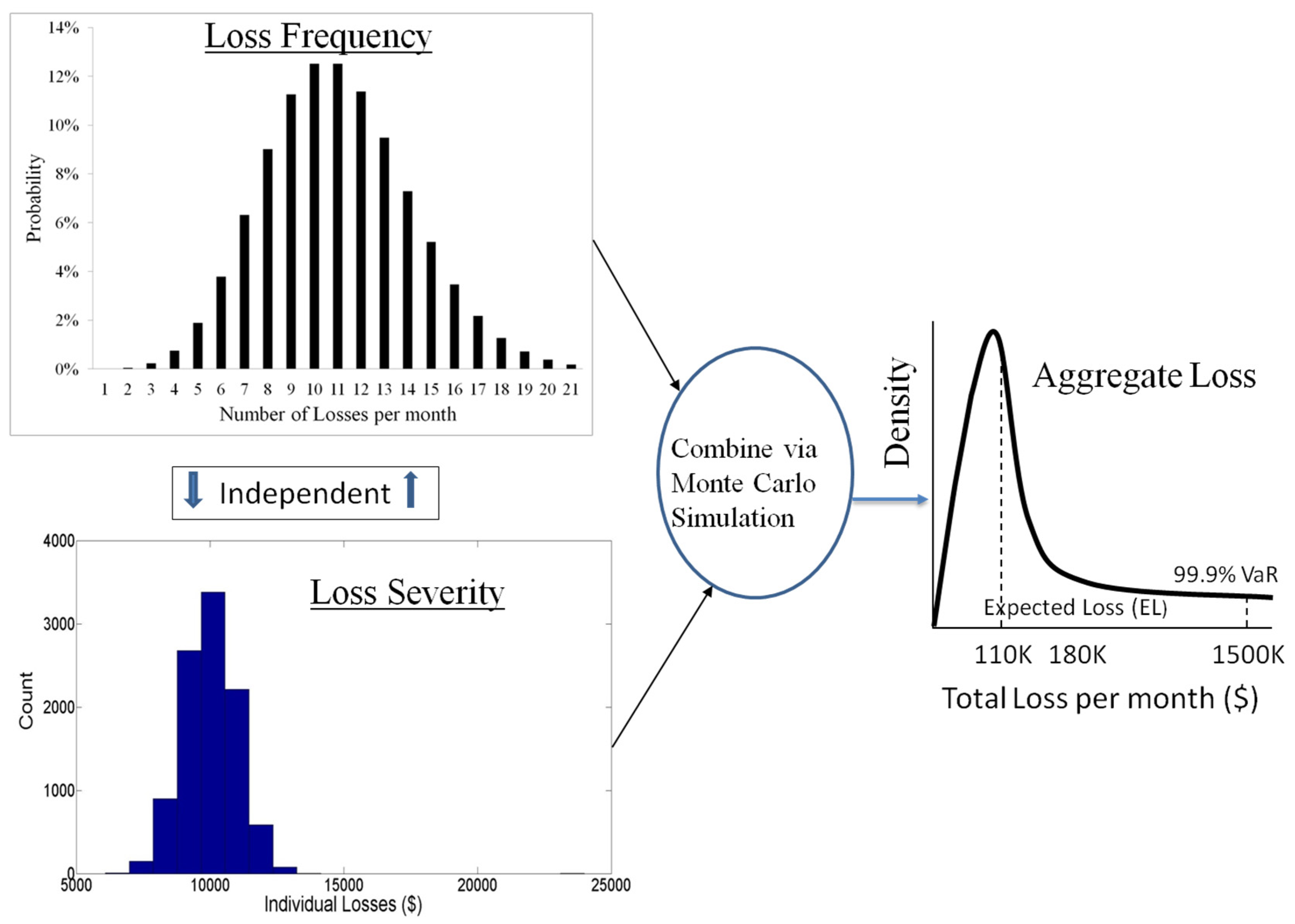
Figure 1. Here we show a visual depiction of the Value-at-Risk (VaR) estimation process using the classical method. By default, the loss frequency and loss severity are independently estimated and the aggregate loss distribution is generated via a Monte Carlo simulation (MCS) to estimate VaR.
Risks 05 00041 g001
Figure 2. Matrix visualization of the split between loss frequency and loss severity in Scenario (I) and (II): (a) The left panel shows Scenario (I) splitting high/medium/low severity → high/medium/low frequency (one-to-many map) (b) The right panel shows Scenario (II): high/medium/low Severity → high/medium/low frequency (one-to-one map). Note, the n/a represents that no relationship exists in that quadrant of the matrix.
Risks 05 00041 g002
Figure 3. Visualization of the loss frequency and loss severity relationship in Scenarios (IV) and (V): (a) Left panel shows Scenario (IV) splitting high/low severity mixture→ high/ low frequency. This case corresponds to the two-regime mixture as described in Section 3.1; (b) The right panel shows Scenario (V), in which a linear relationship exists between frequency and severity. Scenario (IV) represents a mixture relationship between frequency and severity. Scenario (V) depicts a linear functional dependency between frequency and severity.
Risks 05 00041 g003
Figure 4. DPFS for Scenario (I); three distinct regions are found between frequency and severity; centroids are marked with an “x”. The clustering algorithm finds the low severity region which consists of high/medium/low frequencies in Cluster 1 as simulated in Scenario (I). In Cluster 2, the medium severity region consisting of medium/low frequencies is noted by the clustering method. Finally, in Cluster 3, the high severity region consisting of low frequencies only is found.
Risks 05 00041 g004
Figure 5. DPFS Method II applied to simulated Scenario II data. (a) Upper left panel is a histogram of the original loss data (log scale); the other three panels show the split into high (b)/medium (c)/low (d) severity regions. This method correctly identifies the three frequency/severity partitions in Scenario (II): (1) high severity/low frequency region (b); (2) medium severity/medium frequency region (c); (3) low severity/high frequency region (d).
Risks 05 00041 g005
Figure 6. CPFS results: (a) the left panel shows the Gaussian mixture copula model (GMCM) analysis for Scenario (IV); (b) the right panel shows a Gaussian copula analysis for the chemical spills data; red points indicate copula fit, while black are actual data. For both simulated and real-world data, the CPFS method closely fits the real data to the copula function.
Risks 05 00041 g006
Figure 7. VaR estimates by the classical, DPFS and CPFS methods for the simulated Scenario (I) (a) and Scenario (II) (b); DPFS Methods (I) and (II) perform comparable to true VaR while the classical method underestimates the VaR.
Risks 05 00041 g007
Figure 8. VaR estimates by the classical, DPFS and CPFS methods for the simulated Scenario (III); DPFS Methods (I) and (II) perform comparable to true VaR along with the classical method (since frequency is independent of severity); the copula methods overestimate the VaR in these cases. As seen from this figure, the overlapping points corresponding to the DPFS and classical methods indicate that their respective VaR estimates are within 1% of each other and thus visually indistinguishable.
Risks 05 00041 g008
Figure 9. VaR estimates by the classical, DPFS and CPFS methods for the simulated Scenario (IV) (a) and Scenario (V) (b); GMCM performs the best compared to the true VaR, while the K-means and the classical methods underestimate the true VaR in Scenario (IV). For Scenario (V), the t-Copula performs the best for the perfect correlation relationship between frequency and severity.
Risks 05 00041 g009aRisks 05 00041 g009b
Figure 10. VaR estimates by the classical, DPFS, and CPFS methods for the S & P 500 (a) and DJIA data (b). DPFS Methods (I) and (II) works the best compared to the historical bootstrap VaR while the classical methods underestimates the historical bootstrap VaR for Standard & Poor’s (S & P) 500. On the other hand, for the Dow Jones industrial average (DJIA), both DPFS and classical approach estimate the historical bootstrap VaR to within the 99% confidence bands.
Risks 05 00041 g010
Figure 11. VaR estimates by the classical, DPFS and CPFS methods for the Australian automobile accidents data (a); the US hurricanes loss data (b) and chemical spills data (c). The DPFS Method (I) performs the best in estimating VaR for the automobile accident data, while the GMCM method performs best for the hurricanes data. For the chemical spills data, DPFS Method II performs the best compared to the historical bootstrap VaR while the classical method overestimates the historical VaR and is outside the 99% bootstrap confidence bands.
Risks 05 00041 g011
Figure 12. The number of instances when VaR estimation is within 99% bootstrap confidence interval (CI) is plotted versus the magnitude of the correlation ( | ρ * | ) between loss severity and loss frequency for the three methods; namely, classical, CPFS and DPFS. The number of instances is counted using both simulated and real-world datasets. Examining through all of the data sets, we observe three instances where the CPFS methodology accurately estimates the VaR for all of the upper quantiles of the VaR estimate, namely, 90%, 95%, 98%, 99%, 99.5% and 99.9%. Overall, for | ρ * |   40%, the CPFS methodology is the best choice for VaR estimation.
Risks 05 00041 g012
Figure 13. Flow-chart for choosing the VaR estimation method. Here, Freq represents the Frequency component and the 95% CI represents the 95% bootstrap confidence intervals.
Risks 05 00041 g013
Table 1. VaR results for simulated and real-world data; X indicates this method is most accurate in estimating the true VaR; Δ indicates that VaR estimation results are indistinguishable within 1% of each other.
Data TypeVaR Estimation Methodology
DPFSCPFSClassical
Simulated Scenarios DataScenario I: Hi/Med/Low Severity → Hi/Med/Low Frequency (One-to-Many)X
Scenario II: Hi/Med/Low Severity → Hi/Med/Low Frequency (1-to-1)X
Scenario III: Frequency Independent SeverityΔ
Scenario IV: Hi/Low Severity Mixture → Hi/Low Frequency X
Scenario V: Perfect Correlation between Frequency & Severity X
Real-World DataS&P 500X
DJIAΔ
Chemical SpillsX
Automobile AccidentsΔ Δ
US Hurricanes X