Actuarial Applications and Estimation of Extended CreditRisk+

Abstract

We introduce an additive stochastic mortality model which allows joint modelling and forecasting of underlying death causes. Parameter families for mortality trends can be chosen freely. As model settings become high dimensional, Markov chain Monte Carlo is used for parameter estimation. We then link our proposed model to an extended version of the credit risk model CreditRisk${}^{+}$. This allows exact risk aggregation via an efficient numerically stable Panjer recursion algorithm and provides numerous applications in credit, life insurance and annuity portfolios to derive P&L distributions. Furthermore, the model allows exact (without Monte Carlo simulation error) calculation of risk measures and their sensitivities with respect to model parameters for P&L distributions such as value-at-risk and expected shortfall. Numerous examples, including an application to partial internal models under Solvency II, using Austrian and Australian data are shown.

1. Introduction

As the current low interest rate environment forces insurers to put more focus on biometric risks, proper stochastic modelling of mortality has become increasingly important. New regulatory requirements such as Solvency II1 allow the use of internal stochastic models which provide a more risk-sensitive evaluation of capital requirements and the ability to derive accurate profit and loss (P&L) attributions with respect to different sources of risk. Benefits for companies which make use of actuarial tools such as internal models depend crucially on the accuracy of predicted death probabilities and the ability to extract different sources of risk. So far, insurers often use deterministic modelling techniques and then add artificial risk margins to account for risks associated with longevity, size of the portfolio, selection phenomena, estimation and various other sources. Such approaches often lack a stochastic foundation and are certainly not consistently appropriate for all companies.

Deriving P&L distributions of large credit, life and pension portfolios typically is a very challenging task. In applications, Monte Carlo is the most commonly used approach as it is easy to implement for all different kinds of stochastic settings. However, it has shortcomings in finesse and speed, especially for calculation of model sensitivities. Motivated by numerical trials, we found that the credit risk model extended CreditRisk${}^{+}$ (ECRP), as introduced in (Schmock 2017, section 6), is an exceptionally efficient as well as flexible alternative to Monte Carlo and, simultaneously, fits into life actuarial settings as well. Coming from credit risk, this model allows flexible handling of dependence structures within a portfolio via common stochastic risk factors. The ECRP model relies on Panjer recursion (cf. Sundt (1999)) which, unlike Monte Carlo, does not require simulation. It allows an efficient implementation to derive P&L distributions exactly given input data and chosen granularity associated with discretisation. The speed up for deriving sensitivities, i.e., derivatives, of risk measures with respect to model parameters using Panjer recursion will even be an order of magnitude larger as it is extremely difficult to calculate them via finite differencing using Monte Carlo. In addition, our proposed approach can enhance pricing of retirement income products and can be used for applications to partial internal models in the underwriting risk module.

In Section 2 we introduce an additive stochastic mortality model which is related to classical approaches such as the Lee-Carter model introduced in Lee and Carter (1992) or models discussed in Cairns et al. (2009). It allows joint modelling of underlying stochastic death causes based on Poisson assumptions where dependence is introduced via common stochastic risk factors. Note that forecasting of death causes in a disaggregated way can lead to problems with dominating causes in the long run, as argued in Wilmoth (1995) as well as Booth and Tickle (2008). However, joint modelling of death causes can yield computational issues due to high dimensionality which is why the literature is sparse in this matter. An extensive literature review and a multinomial logistic model for joint modelling of death causes is studied in Alai et al. (2015).

Given suitable mortality data, in Section 3 we provide several methods to estimate model parameters including matching of moments, a maximum a posteriori approach and maximum likelihood as well as Markov chain Monte Carlo (MCMC). Death and population data are usually freely available on governmental websites or at statistic bureaus. Due to the high dimensionality of our problem, we suggest the use of MCMC which is one of the few statistical approaches allowing joint parameter estimation in high-dimensions. MCMC can become time-consuming, in particular for settings with common stochastic risk factors. However, estimation of model parameters does usually not have to be done on a frequent basis. We propose a parameter family for mortality trends which makes our model a generalisation of the Lee–Carter approach. However, our approach allows the use of any other kind of parameter family as MCMC is very flexible.

In Section 4 we estimate model parameters for Australian death data in a setting with 362 model parameters, where trends, trend acceleration/reduction and cohort effects are estimated. Further applications include forecasting of central mortality rates and expected future life time.

In Section 5 we then introduce the ECRP model, see (Schmock 2017, section 6), which is a collective risk model corresponding one-to-one to our proposed stochastic mortality model. As the name suggests, it is a credit risk model used to derive loss distributions of credit portfolios and originates from the classical CreditRisk${}^{+}$ model which was introduced by Credit Suisse First Boston (1997). Within credit risk models it is classified as a Poisson mixture model. Identifying default with death makes the model perfectly applicable for actuarial applications. Extended CreditRisk${}^{+}$ provides a flexible basis for modelling multi-level dependencies and allows a fast and numerically stable algorithm for risk aggregation. In the ECRP model, deaths are driven by independent stochastic risk factors. The number of deaths of each policyholder is assumed to be Poisson distributed with stochastic intensity. Thus, serving as an approximation for the true case with single deaths, each person can die multiple times within a period. However, with proper parameter scaling, approximations are very good and final loss distributions are accurate due to Poisson approximation, as shown in Barbour et al. (1992) or Vellaisamy and Chaudhuri (1996) as well as the references therein. The close fit of the ECRP model with (mixed) Poisson distributed deaths to more realistic Bernoulli models is outlined in an introductory example. Another great advantage of the ECRP model is that it automatically incorporates many different sources of risks, such as trends, statistical volatility risk and parameter risk.

Section 6 briefly illustrates validation and model selection techniques. Model validation approaches are based on previously defined dependence and independence structures. All tests suggest that the model suitably fits Australian mortality data.

2. An Alternative Stochastic Mortality Model

2.1. Basic Definitions and Notation

Following standard actuarial notations and definitions, Pitacco et al. (2009) or Cairns et al. (2009), let $T_{a,g}\left(t\right)$ denote the random variable of remaining life time of a person aged $a\in \{0,1,\cdots ,A\}$, with maximum age $A\in \mathbb{N}$, and of gender $g\in \{\mathrm{m},\mathrm{f}\}$ at time/year $t\in \mathbb{N}$. Survival and death probabilities over a time frame $\tau \ge 0$ are given by ${}_{\tau }{p}_{a,g}\left(t\right)=\mathbb{P}(T_{a,g}\left(t\right)>\tau )$ and ${}_{\tau }{q}_{a,g}\left(t\right)=\mathbb{P}(T_{a,g}\left(t\right)\le \tau )$, respectively. For notational purposes we write $q_{a,g}\left(t\right):={}_1{q}_{a,g}\left(t\right)$.

Deterministic force of mortality (theory for the stochastic case is also available) at age $a+\tau$ with gender g of a person aged a at time t is given by the derivative ${\mu }_{a+\tau ,g}\left(t\right):=-\frac{\partial }{\partial \tau }log{}_{\tau }{p}_{a,g}\left(t\right)$. Henceforth, the central death rate of a person aged a at time t and of gender g is given by a weighted average of the force of mortality

$$m_{a,g}\left(t\right):=\frac{{\int }_0^1{}_s{p}_{a,g}(t+s){\mu }_{a+s,g}(t+s)ds}{{\int }_0^1{}_s{p}_{a,g}(t+s)ds}=\frac{q_{a,g}\left(t\right)}{{\int }_0^1{}_s{p}_{a,g}(t+s)ds}\approx \frac{q_{a,g}\left(t\right)}{1-q_{a,g}\left(t\right)/2}.$$

If ${\mu }_{a+s,g}(t+s)={\mu }_{a,g}\left(t\right)$ for all $0\le s<1$ and $a,t\in {\mathbb{N}}_0$ with $a\le A$, i.e., under piecewise constant force of mortality, we have $m_{a,g}\left(t\right)={\mu }_{a,g}\left(t\right)$ as well as $q_{a,g}\left(t\right)=1-exp(-m_{a,g}\left(t\right))$.

Let $N_{a,g}\left(t\right)$ denote the number of recorded deaths in year t of people having age a and gender g, as well as define the exposure to risk $E_{a,g}\left(t\right)$ as the average number of people in year t having age a and gender g. The latter can often be retrieved from statistical bureaus or approximated by the age-dependent population in the middle of a calender year. Estimates for these data in Australia (with several adjustment components such as census undercount and immigration taken into account) are available at the website of the Australian Bureau of Statistics. Considering underlying death causes $k=0,\cdots ,K$, which are to be understood as diseases or injury that initiated the train of morbid events leading directly to death, let $N_{a,g,k}\left(t\right)$ denote the actual number of recorded deaths due to death cause k in year t of people having age a and gender g. Note that $N_{a,g}\left(t\right)=N_{a,g,0}\left(t\right)+\cdots +N_{a,g,K}\left(t\right)$. Data on ICD-classified (short for International Statistical Classification of Diseases and Related Health Problems) death counts can be found for many countries. For Australia these data can be found at the Australian Institute of Health and Welfare (AIHW), classified by ICD-9 and ICD-10.

2.2. Some Classical Stochastic Mortality Models

We start with a simple model and assume that deaths in year t of people having age a and gender g are Poisson distributed $N_{a,g}\left(t\right)\sim \mathrm{Poisson}\left(E_{a,g}\left(t\right)m_{a,g}\left(t\right)\right)$. In this case the maximum likelihood estimate for the central death rate is given by ${\widehat{m}}_{a,g}\left(t\right)={\widehat{N}}_{a,g}\left(t\right)/E_{a,g}\left(t\right)$, where ${\widehat{N}}_{a,g}\left(t\right)$ is the actual recorded number of deaths.

The benchmark stochastic mortality model considered in the literature is the traditional Lee–Carter model, Lee and Carter (1992), where the logarithmic central death rates are modelled in the form

$$log{\widehat{m}}_{a,g}\left(t\right)={\alpha }_{a,g}+{\beta }_{a,g}{\kappa }_t+{\epsilon }_{a,g,t}$$

with independent normal error terms ${\epsilon }_{a,g,t}$ with mean zero, common time-specific component ${\kappa }_t$, as well as age and gender specific parameters ${\alpha }_{a,g}$ and ${\beta }_{a,g}$. Using suitable normalisations, estimates for these parameters and ${\kappa }_t$ can be derived via the method of moments and singular value decompositions, (Kainhofer et al. 2006, section 4.5.1). Forecasts may then be obtained by applying auto-regressive models to ${\kappa }_t$. Note that Fung et al. (2017) and Fung et al. (2015) provide joint estimation of parameters and latent factor ${\kappa }_t$ in the Lee-Carter model via a state-space framework using MCMC. Various extensions of this classical approach with multiple time factors and cohort components have been proposed in the literature; for a review, see Cairns et al. (2009).

Instead of modelling central death rates with normal error terms as in the Lee–Carter approach, Brouhns et al. (2002) propose to model death counts via Poisson regression where error terms are replaced by Poison random variables. In this case $N_{a,g}\left(t\right)\sim \mathrm{Poisson}\left(E_{a,g}\left(t\right)m_{a,g}\left(t\right)\right)$ where, in the simplest case, $log{m}_{a,g}\left(t\right)={\alpha }_{a,g}+{\beta }_{a,g}{\kappa }_t$. Correspondingly, assuming that we want to forecast central death rates for different underlying death causes k, it is natural to assume $N_{a,g,k}\left(t\right)\sim \mathrm{Poisson}\left(E_{a,g}\left(t\right)m_{a,g,k}\left(t\right)\right)$ where $log{m}_{a,g,k}\left(t\right)={\alpha }_{a,g,k}+{\beta }_{a,g,k}{\kappa }_{k,t}$. However, in this case, it is not difficult to see that $m_{a,g,0}\left(t\right)+\cdots +m_{a,g,K}\left(t\right)\ne m_{a,g}\left(t\right)$, in general, and thus

$$\mathbb{E}\left[N_{a,g}\left(t\right)\right]\ne \sum _{k=0}^K\mathbb{E}\left[N_{a,g,k}\left(t\right)\right]$$

since $N_{a,g}\left(t\right)\sim \mathrm{Poisson}\left(E_{a,g}\left(t\right)(m_{a,g,0}\left(t\right)+\cdots +m_{a,g,K}\left(t\right))\right)$. Moreover, as central death rates are increasing for selected underlying death cause (e.g., central death rates for 75–79 year olds in Australia have doubled from 1987 throughout 2011), forecasts increase exponentially, exceeding one in the future.

In light of this shortcoming, we will introduce an additive stochastic mortality model which fits into the risk aggregation framework of extended CredtRisk${}^{+}$, see Schmock (2017).

2.3. An Additive Stochastic Mortality Model

To be able to model different underlying death causes or, more generally, different covariates which show some common death behaviour (however, we will restrict to the first case in this paper), let us assume common stochastic risk factors ${\Lambda }_1\left(t\right),\cdots ,{\Lambda }_K\left(t\right)$ with corresponding age-dependent weights $w_{a,g,k}\left(t\right)$ which give the age-dependent susceptibility to the different risk factors and which satisfy

$$w_{a,g,0}\left(t\right)+\cdots +w_{a,g,K}\left(t\right)=1.$$

Remark 1.

Risk factors introduce dependence amongst deaths of different policyholders. If risk factor ${\Lambda }_k\left(t\right)$ takes large or small values, then the likelihood of death due to k increases or decreases, respectively, simultaneously for all policyholders depending on the weight $w_{a,g,k}\left(t\right)$. Weights $w_{a,g,0},\cdots ,w_{a,g,K}$ indicate the vulnerability of people aged a with gender g to risk factors ${\Lambda }_1\left(t\right),\cdots ,{\Lambda }_K\left(t\right)$. Risk factors are of particular importance to forecast death causes. For a practical example, assume that a new, very effective cancer treatment is available such that fewer people die from lung cancer. This situation would have a longevity effect on all policyholders. Such a scenario would then correspond to the case when the risk factor for neoplasms shows a small realisation.

Definition 1 (Additive stochastic mortality model).

Given risk factors ${\Lambda }_1\left(t\right),\cdots ,{\Lambda }_K\left(t\right)$ with unit mean and variances ${\sigma }_1^2\left(t\right),\cdots ,{\sigma }_K^2\left(t\right)$, assume

$$N_{a,g,k}\left(t\right)\sim \mathrm{Poisson}\left(E_{a,g}\left(t\right)m_{a,g}\left(t\right)w_{a,g,k}\left(t\right){\Lambda }_k\left(t\right)\right),k=1,\cdots ,K,$$

being conditionally independent of all $N_{a,g,k^{\prime }}\left(t\right)$ with $k\ne k^{\prime }$. Idiosyncratic deaths $N_{a,g,0}\left(t\right)$ with $k=0$ are assumed to be mutually independent and independent of all other random variables such that

$$N_{a,g,0}\left(t\right)\sim \mathrm{Poisson}\left(E_{a,g}\left(t\right)m_{a,g}\left(t\right)w_{a,g,0}\left(t\right)\right).$$

In this case, in expectation, deaths due to different underlying death causes add up correctly, i.e.,

$$\mathbb{E}\left[N_{a,g}\left(t\right)\right]=E_{a,g}\left(t\right)m_{a,g}\left(t\right)=E_{a,g}\left(t\right)m_{a,g}\left(t\right)\sum _{k=0}^K{w}_{a,g,k}\left(t\right)=\sum _{k=0}^K\mathbb{E}\left[N_{a,g,k}\left(t\right)\right]$$

as $\mathbb{E}\left[{\Lambda }_k\left(t\right)\right]=1$ by assumption.

Remark 2.

In applications, if $K=0$, it is feasible to replace the Poisson assumption by a more realistic Binomial assumption $N_{a,g,0}\left(t\right)\sim \mathrm{Binomial}\left(E_{a,g}\left(t\right),m_{a,g}\left(t\right)\right)$, as done in Section 4.2 for illustration purposes.

Remark 3.

If risk factors are independent and gamma distributed (as in the case of classical CreditRisk${}^{+}$), then, unconditionally, deaths $N_{a,g,k}\left(t\right)$ have a negative binomial distribution. Then, variance of deaths is given by $\mathrm{Var}\left(N_{a,g,k}\left(t\right)\right)=E_{a,g}\left(t\right)m_{a,g}\left(t\right)w_{a,g,k}\left(t\right)(1+E_{a,g}\left(t\right)m_{a,g}\left(t\right)w_{a,g,k}\left(t\right){\sigma }_k^2\left(t\right))$ with ${\sigma }_k^2\left(t\right)$ denoting the variance of ${\Lambda }_k\left(t\right)$. Analogously, for all $a\ne a^{\prime }$ or $g\ne g^{\prime }$,

$$\mathrm{Cov}(N_{a,g,k}\left(t\right),N_{a^{\prime },g^{\prime },k}\left(t\right))=E_{a,g}\left(t\right)E_{a^{\prime },g^{\prime }}\left(t\right)m_{a,g}\left(t\right)m_{a^{\prime },g^{\prime }}\left(t\right)w_{a,g,k}\left(t\right)w_{a^{\prime },g^{\prime },k}\left(t\right){\sigma }_k^2\left(t\right).$$

(1)

This result will be used in Section 6 for model validation. A similar result also holds for the more general model with dependent risk factors, see (Schmock 2017, section 6.5).

To account for improvement in mortality and shifts in death causes over time, we introduce the following time-dependent parameter families for trends. Similar to the Lee–Carter model, we could simply consider a linear decrease in log mortality. However, since this yields diminishing or exploding mortality over time, we choose a more sophisticated class with trend reduction features. First, in order to guarantee that values lie in the unit interval, let $F^{\mathrm{Lap}}$ denote the Laplace distribution function with mean zero and variance two, i.e.,

$$F^{\mathrm{Lap}}\left(x\right)=\frac{1}{2}+\frac{1}{2}\mathrm{sign}\left(x\right)\left(1-exp(-|x\left|\right)\right),x\in \mathbb{R},$$

such that, for $x<0$, twice the expression becomes the exponential function.

To ensure that weights and death probabilities are strictly positive for $t\to \infty$, we use the trend reduction/acceleration technique

$${\mathcal{T}}_{\zeta ,\eta }^{*}\left(t\right)=\frac{1}{\eta }arctan\left(\eta (t-\zeta )\right),$$

(2)

with parameters $(\zeta ,\eta )\in \mathbb{R}\times (0,\infty )$ and $t\in \mathbb{R}$, which is motivated by (Kainhofer et al. 2006, section 4.6.2). In particular, Equation (2) roughly gives a linear function of t if parameter $\eta$ is small which illustrates the close link to the Lee–Carter model. In order to make estimation more stable, we suggest the normalisation ${\mathcal{T}}_{\zeta ,\eta }\left(t\right)=({\mathcal{T}}_{\zeta ,\eta }^{*}\left(t\right)-{\mathcal{T}}_{\zeta ,\eta }^{*}\left(t_0\right))/({\mathcal{T}}_{\zeta ,\eta }^{*}\left(t_0\right)-{\mathcal{T}}_{\zeta ,\eta }^{*}(t_0-1))$ with normalisation parameter $t_0\in \mathbb{R}$. A clear trend reduction in mortality improvements can be observed in Japan since 1970, see (Pasdika and Wolff 2005, section 4.2), and also for females in Australia.

Definition 2 (Trend families for central death rates and weights).

Central death rates for age a, gender g in year t are given by

$$m_{a,g}\left(t\right)=F^{\mathrm{Lap}}\left({\alpha }_{a,g}+{\beta }_{a,g}{\mathcal{T}}_{{\zeta }_{a,g},{\eta }_{a,g}}\left(t\right)+{\gamma }_{t-a}\right),$$

(3)

with parameters ${\alpha }_{a,g},{\beta }_{a,g},{\zeta }_{a,g},{\gamma }_{t-a}\in \mathbb{R}$ and ${\eta }_i\in (0,\infty )$, as well as where weights are given by

$$w_{a,g,k}\left(t\right)=\frac{exp\left(u_{a,g,k}+v_{a,g,k}{\mathcal{T}}_{{\varphi }_k,{\psi }_k}\left(t\right)\right)}{{\sum }_{j=0}^{K}exp\left(u_{a,g,j}+v_{a,g,j}{\mathcal{T}}_{{\varphi }_j,{\psi }_j}\left(t\right)\right)},k\in \{0,\cdots ,K\},$$

(4)

with parameters $u_{a,g,0},v_{a,g,0},{\varphi }_0,\cdots ,u_{a,g,K},v_{a,g,K},{\varphi }_K\in \mathbb{R}$ and ${\psi }_0,\cdots ,{\psi }_K\in (0,\infty )$.

The assumptions above yield an exponential evolution of central death rates over time, modulo trend reduction ${\mathcal{T}}_{\zeta ,\eta }\left(t\right)$ and cohort effects ${\gamma }_{t-a}$ ($t-a$ refers to the birth year). Vector $\alpha$ can be interpreted as intercept parameter for central death rates. Henceforth, $\beta$ gives the speed of mortality improvement while $\eta$ gives the speed of trend reduction and $\zeta$ gives the shift on the S-shaped arctangent curve, i.e., the location of trend acceleration and trend reduction. Parameter ${\gamma }_{t-a}$ models cohort effects for groups with the same year of birth. This factor can also be understood as a categorical variate such as smoker/non-smoker, diabetic/non-diabetic or country of residence. The interpretation of model parameters for families of weights is similar.

Cohort effects are not used for modelling weights $w_{a,g,k}\left(t\right)$ as sparse data do not allow proper estimation. In applications, we suggest to fix $\varphi$ and $\psi$ in order to reduce dimensionality to suitable levels. Furthermore, fixing trend acceleration/reduction parameters ($\zeta$, $\eta$, $\varphi$, $\psi$) yields stable results over time, with similar behavior as in the Lee-Carter model. Including trend reduction parameters can lead to less stable results over time. However, our proposed model allows free adaption of parameter families for mortality and weights.

Remark 4 (Long-term projections).

Long-term projections of death probabilities using Equation (3) give

$$\underset{t\to \infty }{lim}{m}_{a,g}\left(t\right)=F^{\mathrm{Lap}}\left({\alpha }_{a,g}+{\beta }_{a,g}\frac{\pi }{2{\eta }_{a,g}}\right).$$

Likewise, long-term projections for weights using Equation Equation (4) are given by

$$\underset{t\to \infty }{lim}{w}_{a,g,k}\left(t\right)=\frac{exp\left(u_{a,g,k}+v_{a,g,k}\frac{\pi }{2{\psi }_k}\right)}{{\sum }_{j=0}^{K}exp\left(u_{a,g,j}+v_{a,g,j}\frac{\pi }{2{\psi }_j}\right)}.$$

Thus, given weak trend reduction, i.e., ${\psi }_k$ close to zero, weights with the strongest trend will tend to dominate in the long term. If we a priori fix the parameter for trend reduction ${\psi }_k$ at suitable values, this effect can be controlled. Alternatively, different parameter families for weights can be used, e.g., linear families. Note that our model ensures that weights across risk factors $k=0,1,\cdots ,K$ always sum up to one which is why overall mortality $m_{a,g}\left(t\right)$ is not influenced by weights and their trends.

3. Parameter Estimation

In this section we provide several approaches for parameter estimation in our proposed model from Definitions 1 and 2. The approaches include maximum likelihood, maximum a posteriori, matching of moments and MCMC. Whilst matching of moments estimates are easy to derive but less accurate, maximum a posterior and maximum likelihood estimates cannot be calculated by deterministic numerical optimisation, in general. Thus, we suggest MCMC as a slower but very powerful alternative. Publicly available data based on the whole population of a country are used.

McNeil et al. (2005) in section 8.6 consider statistical inference for Poisson mixture models and Bernoulli mixture models. They briefly introduce moment estimators and maximum likelihood estimators for homogeneous groups in Bernoulli mixture models. Alternatively, they derive statistical inference via a generalised linear mixed model representation for mixture models which is distantly related to our setting. In their ‘Notes and Comments’ section the reader can find a comprehensive list of interesting references. Nevertheless, most of their results and arguments are not directly applicable to our case since we use a different parametrisation and since we usually have rich data of death counts compared to the sparse data on company defaults.

In order to be able to derive statistically sound estimates, we make the following simplifying assumption for time independence:

Definition 3 (Time independence and risk factors).

Given Definition 1, consider discrete-time periods $U:=\{1,\cdots ,T\}$ and assume that random variables are independent for different points in time $s\ne t$ in U. Moreover, for each $t\in U$, risk factors ${\Lambda }_1\left(t\right),\cdots ,{\Lambda }_K\left(t\right)$ are assumed to be independent and, for each $k\in \{1,\cdots ,K\}$, ${\Lambda }_k\left(1\right),\cdots ,{\Lambda }_k\left(T\right)$ are identically gamma distributed with mean one and variance ${\sigma }_k^2\ge 0$.

The assumptions made above seem suitable for Austrian and Australian data, as shown in Section 6 via model validation. In particular, serial dependence is mainly captured by trend families in death probabilities and weights.

For estimation of life tables we usually assume $K=0$ or $K=1$ with $w_{a,g,1}=1$ for all ages and genders. For estimation and forecasting of death causes, we identify risk factors with underlying death causes. Note that for fixed a and g, Equation (4) is invariant under a constant shift of parameters ${\left(u_{\mathrm{a},\mathrm{g},k}\right)}_{k\in \{0,\cdots ,K\}}$ as well as ${\left(v_{\mathrm{a},\mathrm{g},k}\right)}_{k\in \{0,\cdots ,K\}}$ if ${\varphi }_0=\cdots ={\varphi }_K$ and ${\psi }_0=\cdots ={\psi }_K$, respectively. Thus, for each a and g, we can always choose fixed and arbitrary values for $u_{a,g,0}$ and $v_{a,g,0}$.

3.1. Estimation via Maximum Likelihood

We start with the classical maximum likelihood approach. The likelihood function can be derived in closed form but, unfortunately, estimates have to be derived via MCMC as deterministic numerical optimisation quickly breaks down due to high dimensionality.

Lemma 1 (Likelihood function).

Given Definitions 1–3, define

$${\widehat{N}}_k\left(t\right):=\sum _{a=0}^A\sum _{g\in \{\mathrm{f},\mathrm{m}\}}{\widehat{N}}_{a,g,k}\left(t\right),k\in \{0,\cdots ,K\}andt\in U,$$

as well as ${\rho }_{a,g,k}\left(t\right):=E_{a,g}\left(t\right)m_{a,g}\left(t\right)w_{a,g,k}\left(t\right)$ for all age groups a, with maximum age group A, and gender g and

$${\rho }_k\left(t\right):=\sum _{a=0}^A\sum _{g\in \{\mathrm{f},\mathrm{m}\}}{\rho }_{a,g,k}\left(t\right).$$

Then, the likelihood function $\ell (\widehat{N}|{\theta }_m,{\theta }_w,\sigma )$ of parameters ${\theta }_m:=(\alpha ,\beta ,\zeta ,\eta )\in E$, as well as ${\theta }_w:=(u,v,\varphi ,\psi )\in F$ and $\sigma :=\left({\sigma }_k\right)\in {[0,\infty )}^K$ given $\widehat{N}:=({\widehat{N}}_{a,g,k}\left(t\right))\in {\mathbb{N}}_0^{A\times 2\times (K+1)\times T}$ is given by

$$\begin{array}{c}\ell (\widehat{N}|{\theta }_m,{\theta }_w,\sigma )=\prod _{t=1}^T(\left(\prod _{a=0}^A\prod _{g\in \{\mathrm{f},\mathrm{m}\}}\frac{e^{-{\rho }_{a,g,0}\left(t\right)}{\rho }_{a,g,0}{\left(t\right)}^{{\widehat{N}}_{a,g,0}\left(t\right)}}{{\widehat{N}}_{a,g,k}\left(t\right)!}\right)\\ \times \prod _{k=1}^K\left(\frac{\Gamma ({\sigma }_k^{-2}+{\widehat{N}}_k\left(t\right))}{\Gamma ({\sigma }_k^{-2}){\sigma }_k^{2{\sigma }_k^{-2}}{({\sigma }_k^{-2}+{\rho }_k\left(t\right))}^{{\sigma }_k^{-2}+{\widehat{N}}_k\left(t\right)}}\prod _{a=0}^A\prod _{g\in \{\mathrm{f},\mathrm{m}\}}\frac{{\rho }_{a,g,k}{\left(t\right)}^{{\widehat{N}}_{a,g,k}\left(t\right)}}{{\widehat{N}}_{a,g,k}\left(t\right)!}\right)).\end{array}$$

(5)

Proof. 

Following our assumptions, by straightforward computation we get

$$\begin{array}{c}\ell (\widehat{N}|{\theta }_m,{\theta }_w,\sigma )=\prod _{t=1}^T(\left(\prod _{a=0}^A\prod _{g\in \{\mathrm{f},\mathrm{m}\}}\frac{e^{-{\rho }_{a,g,0}\left(t\right)}{\rho }_{a,g,0}{\left(t\right)}^{{\widehat{N}}_{a,g,0}\left(t\right)}}{{\widehat{N}}_{a,g,0}\left(t\right)!}\right)\\ \times \prod _{k=1}^K\mathbb{E}\left[\mathbb{P}\left(\bigcap _{a=0}^A\bigcap _{g\in \{\mathrm{f},\mathrm{m}\}}\left\{N_{a,g,k}\left(t\right)={\widehat{N}}_{a,g,k}\left(t\right)\right\}|{\Lambda }_k\left(t\right)\right)\right]),\end{array}$$

where $\ell (\widehat{N}|{\theta }_m,{\theta }_w,\sigma )=\mathbb{P}(N=\widehat{N}|{\theta }_m,{\theta }_w,\sigma )$ denotes the probability of the event $\{N=\widehat{N}\}$ given parameters. Taking expectations in the equation above yields

$$\begin{array}{cc}\hfill \mathbb{E}& [\mathbb{P}\left(\bigcap _{a=0}^A\bigcap _{g\in \{\mathrm{f},\mathrm{m}\}}\left\{N_{a,g,k}\left(t\right)={\widehat{N}}_{a,g,k}\left(t\right)\right\}|{\Lambda }_k\left(t\right)\right)]\hfill \\ & =\left(\prod _{a=0}^A\prod _{g\in \{\mathrm{f},\mathrm{m}\}}\frac{{\rho }_{a,g,k}{\left(t\right)}^{{\widehat{N}}_{a,g,k}\left(t\right)}}{{\widehat{N}}_{a,g,k}\left(t\right)!}\right){\int }_0^{\infty }{e}^{-{\rho }_k\left(t\right)x_t}{x}_t^{{\widehat{N}}_k\left(t\right)}\frac{x_t^{{\sigma }_k^{-2}-1}{e}^{-x_t{\sigma }_k^{-2}}}{\Gamma \left({\sigma }_k^{-2}\right){\sigma }_k^{2{\sigma }_k^{-2}}}d{x}_t.\hfill \end{array}$$

The integrand above is a density of a gamma distribution—modulo the normalisation constant—with parameters ${\sigma }_k^{-2}+{\widehat{N}}_k\left(t\right)$ and ${\sigma }_k^{-2}+{\rho }_k\left(t\right)$. Therefore, the corresponding integral equals the multiplicative inverse of the normalisation constant, i.e.,

$$\begin{array}{c}\hfill {\left(\frac{{({\sigma }_k^{-2}+{\rho }_k\left(t\right))}^{{\sigma }_k^{-2}+{\widehat{N}}_k\left(t\right)}}{\Gamma ({\sigma }_k^{-2}+{\widehat{N}}_k\left(t\right))}\right)}^{-1},k\in \{1,\cdots ,K\}\mathrm{and}t\in \{1,\cdots ,T\}.\end{array}$$

Putting all results together gives Equation (5). ☐

Since the products in Equation (5) can become small, we recommend to use the log-likelihood function instead. For implementations we recommend to use the log-gamma function, e.g., the lgamma function in ‘R’ see R Core Team (2013).

Definition 4 (Maximum likelihood estimates).

Recalling Equation (5), as well as given the assumptions of Lemma 1, maximum likelihood estimates for parameters ${\theta }_m,{\theta }_w$ and σ are defined by

$$\left({\widehat{\theta }}_m^{\mathrm{MLE}},{\widehat{\theta }}_w^{\mathrm{MLE}},{\widehat{\sigma }}^{\mathrm{MLE}}\right):=\underset{{\theta }_m,{\theta }_w,\sigma }{\arg \sup }\ell (\widehat{N}|{\theta }_m,{\theta }_w,\sigma )=\underset{{\theta }_m,{\theta }_w,\sigma }{\arg \sup }log\ell (\widehat{N}|{\theta }_m,{\theta }_w,\sigma ).$$

Deterministic optimisation of the likelihood function may quickly lead to numerical issues due to high dimensionality. In ‘R’ the deterministic optimisation routine nlminb, see R Core Team (2013), gives stable results in simple examples. Our proposed alternative is to switch to a Bayesian setting and use MCMC as described in Section 3.3.

3.2. Estimation via a Maximum a Posteriori Approach

Secondly we propose a variation of maximum a posteriori estimation based on Bayesian inference, (Shevchenko 2011, section 2.9). If risk factors are not integrated out in the likelihood function, we may also derive the posterior density of the risk factors as follows. One main advantage of this approach is that estimates for risk factors are obtained which is very useful for scenario analysis and model validation. Furthermore, handy approximations for estimates of risk factor realisations and variances are obtained.

Lemma 2 (Posterior density).

Given Definitions 1–3, consider parameters ${\theta }_m:=(\alpha ,\beta ,\zeta ,\eta )\in E$, ${\theta }_w:=(u,v,\varphi ,\psi )\in F$, as well as realisations $\lambda :=\left({\lambda }_k\left(t\right)\right)\in {(0,\infty )}^{K\times T}$ of risk factors $\Lambda :=\left({\Lambda }_k\left(t\right)\right)\in {(0,\infty )}^{K\times T}$, as well as data $\widehat{N}:=({\widehat{N}}_{a,g,k}\left(t\right))\in {\mathbb{N}}_0^{A\times 2\times (K+1)\times T}$. Assume that their prior distribution is denoted by $\pi ({\theta }_m,{\theta }_w,\sigma )$. Then, the posterior density $\pi ({\theta }_m,{\theta }_w,\lambda ,\sigma |\widehat{N})$ of parameters given data $\widehat{N}$ is up to constant given by

$$\begin{array}{cc}\hfill \pi & ({\theta }_m,{\theta }_w,\lambda ,\sigma |\widehat{N})\propto \pi ({\theta }_m,{\theta }_w,\sigma )\pi (\lambda |{\theta }_m,{\theta }_w,\sigma )\ell (\widehat{N}|{\theta }_m,{\theta }_w,\lambda ,\sigma )\hfill \\ & =\prod _{t=1}^T\left(\left(\prod _{a=0}^A\prod _{g\in \{\mathrm{f},\mathrm{m}\}}\frac{e^{-{\rho }_{a,g,0}\left(t\right)}{\rho }_{a,g,0}{\left(t\right)}^{{\widehat{N}}_{a,g,0}\left(t\right)}}{{\widehat{N}}_{a,g,0}\left(t\right)!}\right)\prod _{k=1}^K\right(\frac{e^{-{\lambda }_k\left(t\right){\sigma }_k^{-2}}{\lambda }_k{\left(t\right)}^{{\sigma }_k^{-2}-1}}{\Gamma \left({\sigma }_k^{-2}\right){\sigma }_k^{2{\sigma }_k^{-2}}}\hfill \\ & \times \prod _{a=0}^A\prod _{g\in \{\mathrm{f},\mathrm{m}\}}\frac{e^{-{\rho }_{a,g,k}\left(t\right){\lambda }_k\left(t\right)}{\left({\rho }_{a,g,k}\left(t\right){\lambda }_k\left(t\right)\right)}^{{\widehat{N}}_{a,g,k}\left(t\right)}}{{\widehat{N}}_{a,g,k}\left(t\right)!}\left)\right)\pi ({\theta }_m,{\theta }_w,\sigma ),\hfill \end{array}$$

(6)

where $\pi (\lambda |{\theta }_m,{\theta }_w,\sigma )$ denotes the prior distribution of risk factors at $\Lambda =\lambda$ given all other parameters, where $\ell (\widehat{N}|{\theta }_m,{\theta }_w,\lambda ,\sigma )$ denotes the likelihood of $N=\widehat{N}$ given all parameters and where ${\rho }_{a,g,k}\left(t\right)=E_{a,g}\left(t\right)m_{a,g}\left(t\right)w_{a,g,k}\left(t\right)$.

Proof. 

The first proportional equality follows by Bayes’ theorem which is also widely used in Bayesian inference, see, for example, (Shevchenko 2011, section 2.9). Moreover,

$$\pi (\lambda |{\theta }_m,{\theta }_w,\sigma )=\prod _{k=1}^K\prod _{t=1}^T\left(\frac{e^{-{\lambda }_k\left(t\right){\sigma }_k^{-2}}{\lambda }_k{\left(t\right)}^{{\sigma }_k^{-2}-1}}{\Gamma \left({\sigma }_k^{-2}\right){\sigma }_k^{2{\sigma }_k^{-2}}}\right).$$

If ${\theta }_m\in E$, ${\theta }_w\in F$, $\lambda \in {(0,\infty )}^{K\times T}$ and $\sigma \in {[0,\infty )}^K$, then note that

$$\begin{array}{cc}\hfill \ell (\widehat{N}|{\theta }_m,{\theta }_w,\lambda ,\sigma )& =\prod _{a=0}^A\prod _{g\in \{\mathrm{f},\mathrm{m}\}}\prod _{t=1}^T(e^{-{\rho }_{a,g,0}\left(t\right)}\frac{{\rho }_{a,g,0}{\left(t\right)}^{{\widehat{N}}_{a,g,0}\left(t\right)}}{{\widehat{N}}_{a,g,0}\left(t\right)!}\hfill \\ & \times \prod _{k=1}^K\mathbb{P}\left(N_{a,g,k}\left(t\right)={\widehat{N}}_{a,g,k}\left(t\right)|{\Lambda }_k\left(t\right)={\lambda }_k\left(t\right)\right)),\hfill \end{array}$$

which then gives Equation (6) by straightforward computation as in Lemma 1. ☐

The approach described above may look like a pure Bayesian inference approach but note that risk factors ${\Lambda }_k\left(t\right)$ are truly stochastic and, therefore, we refer to it as a maximum a posteriori estimation approach. There are many reasonable choices for prior distributions of parameters which include (improper) uniform priors $\pi ({\theta }_m,{\theta }_w,\sigma ):=1_E\left({\theta }_m\right)1_F\left({\theta }_w\right)1_{{(0,\infty )}^K}\left(\sigma \right)$ to smoothing priors as given in Section 4.2. Having derived the posterior density, we can now define corresponding maximum a posteriori estimates.

Definition 5 (Maximum a posteriori estimates).

Recalling Equation (6), as well as given the assumptions of Lemma 2, maximum a posteriori estimates for parameters ${\theta }_m,{\theta }_w,\lambda$ and σ, given uniqueness, are defined by

$$\left({\widehat{\theta }}_m^{\mathrm{MAP}},{\widehat{\theta }}_w^{\mathrm{MAP}},{\widehat{\lambda }}^{\mathrm{MAP}},{\widehat{\sigma }}^{\mathrm{MAP}}\right):=\underset{{\theta }_m,{\theta }_w,\lambda ,\sigma }{\arg \sup }\pi ({\theta }_m,{\theta }_w,\lambda ,\sigma |\widehat{N})=\underset{{\theta }_m,{\theta }_w,\lambda ,\sigma }{\arg \sup }log\pi ({\theta }_m,{\theta }_w,\lambda ,\sigma |\widehat{N}).$$

Again, deterministic optimisation of the posterior function may quickly lead to numerical issues due to high dimensionality of the posterior function which is why we recommend MCMC. However, we can provide handy approximations for risk factor and variance estimates.

Lemma 3 (Conditions for maximum a posteriori estimates).

Given Definition 5, estimates ${\widehat{\lambda }}^{\mathrm{MAP}}$ and ${\widehat{\sigma }}^{\mathrm{MAP}}$ satisfy, for every $k\in \{1,\cdots ,K\}$ and $t\in U$,

$${\widehat{\lambda }}_k^{\mathrm{MAP}}\left(t\right)=\frac{{({\widehat{\sigma }}_k^{\mathrm{MAP}})}^{-2}-1+{\sum }_{a=0}^A{\sum }_{g\in \{\mathrm{f},\mathrm{m}\}}{\widehat{N}}_{a,g,k}\left(t\right)}{{({\widehat{\sigma }}_k^{\mathrm{MAP}})}^{-2}+{\sum }_{a=0}^A{\sum }_{g\in \{\mathrm{f},\mathrm{m}\}}{\rho }_{a,g,k}\left(t\right)}$$

(7)

if ${({\widehat{\sigma }}_k^{\mathrm{MAP}})}^{-2}-1+{\sum }_{a=0}^A{\sum }_{g\in \{\mathrm{f},\mathrm{m}\}}{\widehat{N}}_{a,g,k}\left(t\right)>0$, as well as

$$2log{\widehat{\sigma }}_k^{\mathrm{MAP}}+\frac{{\Gamma }^{\prime }\left({({\widehat{\sigma }}_k^{\mathrm{MAP}})}^{-2}\right)}{\Gamma \left({({\widehat{\sigma }}_k^{\mathrm{MAP}})}^{-2}\right)}=\frac{1}{T}\sum _{t=1}^T\left(1+log{\widehat{\lambda }}_k^{\mathrm{MAP}}\left(t\right)-{\widehat{\lambda }}_k^{\mathrm{MAP}}\left(t\right)\right),$$

(8)

where, for given ${\widehat{\lambda }}_k^{\mathrm{MAP}}\left(1\right),\cdots ,{\widehat{\lambda }}_k^{\mathrm{MAP}}\left(T\right)>0$, Equation (8) has a unique solution which is strictly positive.

Proof. 

First, set ${\pi }^{*}(\widehat{N}):=log\pi ({\theta }_m,{\theta }_w,\lambda ,\sigma |\widehat{N})$. Then, for every $k\in \{1,\cdots ,K\}$ and $t\in U$, differentiating ${\pi }^{*}(\widehat{N})$ gives

$$\frac{\partial {\pi }^{*}(\widehat{N})}{\partial {\lambda }_k\left(t\right)}=\frac{{\sigma }_k^{-2}-1}{{\lambda }_k\left(t\right)}-\frac{1}{{\sigma }_k^2}+\sum _{a=0}^A\sum _{g\in \{\mathrm{f},\mathrm{m}\}}\left(\frac{{\widehat{N}}_{a,g,k}\left(t\right)}{{\lambda }_k\left(t\right)}-{\rho }_{a,g,k}\left(t\right)\right).$$

Setting this term equal to zero and solving for ${\Lambda }_k\left(t\right)$ gives Equation (7). Similarly, for every $k\in \{1,\cdots ,K\}$, we obtain

$$\frac{\partial {\pi }^{*}(\widehat{N})}{\partial {\sigma }_k^2}=\frac{1}{{\sigma }_k^4}\sum _{t=1}^T\left(log{\sigma }_k^2-1+\frac{{\Gamma }^{\prime }({\sigma }_k^{-2})}{\Gamma ({\sigma }_k^{-2})}-log{\lambda }_k\left(t\right)+{\lambda }_k\left(t\right)\right).$$

Again, setting this term equal to zero and rearranging the terms gives Equation (8).

For existence and uniqueness of the solution in Equation (8), consider ${\widehat{\lambda }}_k^{\mathrm{MAP}}\left(1\right),\cdots ,{\widehat{\lambda }}_k^{\mathrm{MAP}}\left(T\right)>0$ and let $k\in \{1,\cdots ,K\}$ be fixed. Then, note that the right side in Equation (8) is strictly negative unless ${\widehat{\lambda }}_k^{\mathrm{MAP}}\left(1\right)=\cdots ={\widehat{\lambda }}_k^{\mathrm{MAP}}\left(T\right)=1$, as $logx\le x-1$ for all $x>0$ with equality for $x=1$. If ${\widehat{\lambda }}_k^{\mathrm{MAP}}\left(1\right)=\cdots ={\widehat{\lambda }}_k^{\mathrm{MAP}}\left(T\right)=1$, then there is no variability in the risk factor such that ${\sigma }_k^2=0$. Henceforth, note that $f\left(x\right):=logx-{\Gamma }^{\prime }\left(x\right)/\Gamma \left(x\right)$, for all $x>0$, is continuous (${\Gamma }^{\prime }\left(x\right)/\Gamma \left(x\right)$ is known as digamma function or $\psi$-function) with

$$\frac{1}{2x}<f\left(x\right)<\frac{1}{2x}+\frac{1}{12x^2},x>0,$$

(9)

which follows by (Qi et al. 2005, Corollary 1) and $f(x+1)=1/x+f\left(x\right)$ for all $x>0$. As we want to solve $-f(1/x)=-c$ for some given $c>0$, note that $f(0+)=\infty$, as well as ${lim}_{x\to \infty }f\left(x\right)=0$. Thus, a solution has to exist as $f(1/x)$ is continuous on $x>0$. Furthermore,

$$f^{\prime }\left(x\right)=\frac{1}{x}-\sum _{i=0}^{\infty }\frac{1}{{(x+i)}^2}<\frac{1}{x}-{\int }_x^{\infty }\frac{1}{z^2}dz=0,x>0,$$

where the first equality follows by Chaudhry and Zubair (2001). This implies that $f\left(x\right)$ and $(-f(1/x\left)\right)$ are strictly decreasing. Thus, the solution in (8) is unique. ☐

Using Lemma 3, it is possible to derive handy approximations for risk factor and variance estimates, given estimates for weights and death probabilities which can be derived by matching of moments as given in Section 3.4 or other models such as Lee–Carter. If ${\sum }_{a=0}^A{\sum }_{g\in \{\mathrm{f},\mathrm{m}\}}{\widehat{N}}_{a,g,k}\left(t\right)$ is large, it is reasonable to define

$${\widehat{\lambda }}_k^{\mathrm{MAPappr}}\left(t\right):=\frac{-1+{\sum }_{a=0}^A{\sum }_{g\in \{\mathrm{f},\mathrm{m}\}}{\widehat{N}}_{a,g,k}\left(t\right)}{{\sum }_{a=0}^A{\sum }_{g\in \{\mathrm{f},\mathrm{m}\}}{\rho }_{a,g,k}\left(t\right)}$$

(10)

as an approximative estimate for ${\lambda }_k\left(t\right)$ where ${\rho }_{a,g,k}\left(t\right):=E_{a,g}\left(t\right)m_{a,g}\left(t\right)w_{a,g,k}\left(t\right)$. Having derived approximations for $\lambda$, we can use Equation (8) to get estimates for $\sigma$. Alternatively, note that due to Equation (9), we get

$$-2log{\widehat{\sigma }}_k^{\mathrm{MAP}}-\frac{{\Gamma }^{\prime }\left({({\widehat{\sigma }}_k^{\mathrm{MAP}})}^{-2}\right)}{\Gamma \left({({\widehat{\sigma }}_k^{\mathrm{MAP}})}^{-2}\right)}=\frac{{({\widehat{\sigma }}_k^{\mathrm{MAP}})}^2}{2}+\mathcal{O}\left({({\widehat{\sigma }}_k^{\mathrm{MAP}})}^4\right).$$

Furthermore, if we use second order Taylor expansion for the logarithm, then the right hand side of Equation (8) gets

$$\frac{1}{T}\sum _{t=1}^T\left({\widehat{\lambda }}_k^{\mathrm{MAP}}\left(t\right)-1-log{\widehat{\lambda }}_k^{\mathrm{MAP}}\left(t\right)\right)=\frac{1}{2T}\sum _{t=1}^T\left({\left({\widehat{\lambda }}_k^{\mathrm{MAP}}\left(t\right)-1\right)}^2+\mathcal{O}\left({\left({\widehat{\lambda }}_k^{\mathrm{MAP}}\left(t\right)-1\right)}^3\right)\right).$$

This approximation is better the closer the values of $\lambda$ are to one. Thus, using these observations, an approximation for risk factor variances ${\sigma }^2$ is given by

$${\left({\widehat{\sigma }}_k^{\mathrm{MAPappr}}\right)}^2:=\frac{1}{T}\sum _{t=1}^T{\left({\widehat{\lambda }}_k^{\mathrm{MAPappr}}\left(t\right)-1\right)}^2,$$

(11)

which is simply the sample variance of ${\widehat{\lambda }}^{\mathrm{MAP}}$. Note that $|{\widehat{\lambda }}_k^{\mathrm{MAP}}\left(t\right)-1|<|{\widehat{\lambda }}_k^{\mathrm{MAPappr}}\left(t\right)-1|$, implying that Equation (11) will dominate solutions obtained by Equation (8) in most cases.

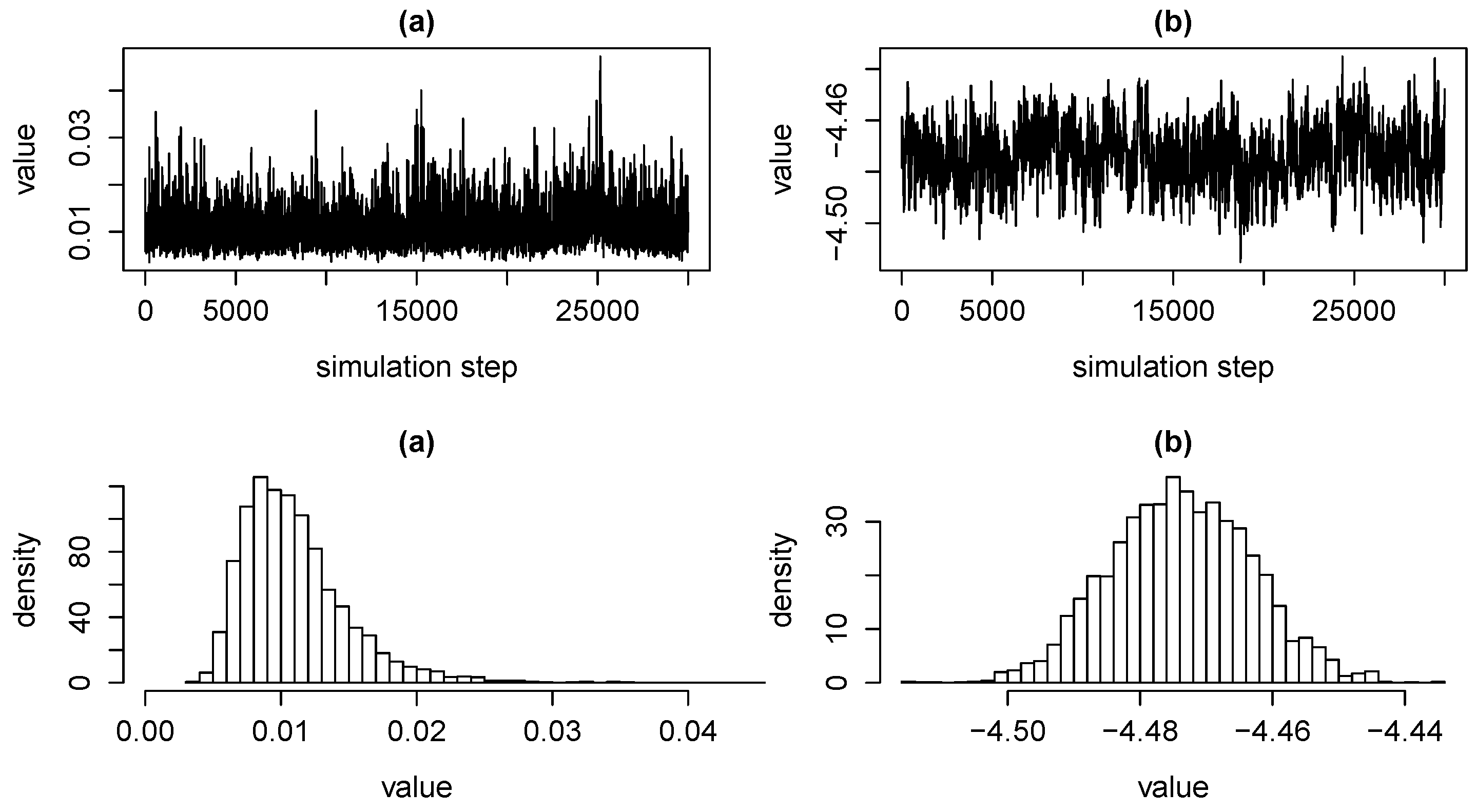
3.3. Estimation via MCMC

As we have already outlined in in the previous sections, deriving maximum a posteriori estimates and maximum likelihood estimates via deterministic numerical optimisation is mostly impossible due to high dimensionality (several hundred parameters). Alternatively, we can use MCMC under a Bayesian setting. Introductions to this topic can be found, for example, in Gilks (1995), Gamerman and Lopes (2006), as well as (Shevchenko 2011, section 2.11). We suggest to use the random walk Metropolis–Hastings within Gibbs algorithm which, given that the Markov chain is irreducible and aperiodic, generates sample chains that converge to the stationary distribution, Tierney (1994) and also (Robert and Casella 2004, sections 6–10). However, note that various MCMC algorithms are available.

MCMC requires a Bayesian setting which we automatically have in the maximum a posteriori approach, see Section 3.2. Similarly, we can switch to a Bayesian setting in the maximum likelihood approach, see Section 3.1, by simply multiplying the likelihood function with a prior distribution of parameters. MCMC generates Markov chains which provide samples from the posterior distribution where the mode of these samples then corresponds to an approximation for the maximum a posteriori estimate. More stable estimates in terms of mean squared error are obtained by taking the mean over all samples once MCMC chains sample from the stationary distribution, (Shevchenko 2011, section 2.10). Taking the mean over all samples as an estimate, of course, can lead to troubles if posterior distributions of parameters are, e.g., bimodal, such that we end up in a region which is highly unlikely. Furthermore, sampled posterior distribution can be used to estimate parameter uncertainty. The method requires a certain burn-in period until the generated chain becomes stationary. Typically, one tries to get average acceptance probabilities close to $0.234$ which is asymptotically optimal for multivariate Gaussian proposals as shown in Roberts et al. (1997). To reduce long computational times, one can run several independent MCMC chains with different starting points on different CPUs in a parallel way. To prevent overfitting, it is possible to regularise, i.e., smooth, maximum a posteriori estimates via adjusting the prior distribution. This technique is particularly used in regression, as well as in many applications, such as signal processing. When forecasting death probabilities in Section 4.2, we use a Gaussian prior density with a certain correlation structure.

Also under MCMC, note that ultimately we are troubled with the curse of dimensionality as we will never be able to get an accurate approximation of the joint posterior distribution in a setting with several hundred parameters.

As MCMC samples yield confidence bands for parameter estimates, they can easily be checked for significance at every desired level, i.e., parameters are not significant if confidence bands cover the value zero. In our subsequent examples, almost all parameters are significant. Given internal mortality data, these confidence bands for parameter estimates can also be used to test whether parameters significantly deviate from officially published life tables. On the other hand, MCMC is perfectly applicable to sparse data as life tables can be used as prior distributions with confidence bands providing an estimate for parameter uncertainty which increase with fewer data points.

3.4. Estimation via Matching of Moments

Finally, we provide a matching of moments approach which allows easier estimation of parameters but which is less accurate. Therefore, we suggest this approach solely to be used to obtain starting values for the other, more sophisticated estimation procedures. In addition, matching of moments approach needs simplifying assumptions to guarantee independent and identical random variables over time.

Assumption 1 (i.i.d. setting).

Given Definitions 1–3, assume death counts ${\left(N_{a,g,k}\left(t\right)\right)}_{t\in U}$ to be i.i.d. with $E_{a,g}:=E_{a,g}\left(1\right)=\cdots =E_{a,g}\left(T\right)$ and $m_{a,g}:=m_{a,g}\left(1\right)=\cdots =m_{a,g}\left(T\right)$, as well as $w_{a,g,k}:=w_{a,g,k}\left(1\right)=\cdots =w_{a,g,k}\left(T\right)$.

To achieve such an i.i.d. setting, transform deaths $N_{a,g,k}\left(t\right)$ such that Poisson mixture intensities are constant over time via

$$N_{a,g,k}^{\prime }\left(t\right):=⌊\frac{E_{a,g}\left(T\right)m_{a,g}\left(T\right)w_{a,g,k}\left(T\right)}{E_{a,g}\left(t\right)m_{a,g}\left(t\right)w_{a,g,k}\left(t\right)}{N}_{a,g,k}\left(t\right)⌋,t\in U,$$

and, correspondingly, define $E_{a,g}:=E_{a,g}\left(T\right)$, as well as $m_{a,g}:=m_{a,g}\left(T\right)$ and $w_{a,g,k}:=w_{a,g,k}\left(T\right)$. Using this modification, we manage to remove long term trends and keep $E_{a,g}\left(t\right)$, $m_{a,g}\left(t\right)$ and $w_{a,g,k}\left(t\right)$ constant over time.

Estimates ${\widehat{m}}_{a,g}^{\mathrm{MM}}\left(t\right)$ for central death rates $m_{a,g}\left(t\right)$ can be obtained via minimising mean squared error to crude death rates which, if parameters $\zeta$, $\eta$ and $\gamma$ are previously fixed, can be obtained by regressing

$${\left(F^{\mathrm{Lap}}\right)}^{-1}\left(\frac{{\sum }_{k=0}^K{\widehat{N}}_{a,g,k}^{\prime }\left(t\right)}{E_{a,g}}\right)-{\gamma }_{a-t}$$

on ${\mathcal{T}}_{{\zeta }_{a,g},{\eta }_{a,g}}\left(t\right)$. Estimates ${\widehat{u}}_{a,g,k}^{\mathrm{MM}},{\widehat{v}}_{a,g,k}^{\mathrm{MM}},{\widehat{\varphi }}_k^{\mathrm{MM}},{\widehat{\psi }}_k^{\mathrm{MM}}$ for parameters $u_{a,g,k},v_{a,g,k},{\varphi }_k,{\psi }_k$ via minimising the mean squared error to crude death rates which again, if parameters $\varphi$ and $\psi$ are previously fixed, can be obtained by regressing $log({\widehat{N}}_{a,g,k}^{\prime }\left(t\right))-log(E_{a,g}{\widehat{m}}_{a,g}^{\mathrm{MM}}\left(t\right))$ on ${\mathcal{T}}_{{\varphi }_k,{\psi }_k}\left(t\right)$. Estimates ${\widehat{w}}_{a,g,k}^{\mathrm{MM}}\left(t\right)$ are then given by Equation (4).

Then, define unbiased estimators for weights $W_{a,g,k}^{*}\left(t\right):=N_{a,g,k}^{\prime }\left(t\right)/E_{a,g}{m}_{a,g}$, as well as

$${\overline{W}}_{a,g,k}^{*}:=\frac{1}{T}\sum _{t=1}^T{W}_{a,g,k}^{*}\left(t\right).$$

In particular, we have $\mathbb{E}[{\overline{W}}_{a,g,k}^{*}]=\mathbb{E}[W_{a,g,k}^{*}\left(t\right)]=w_{a,g,k}$.

Lemma 4.

Given Assumptions 3, define

$${\widehat{\Sigma }}_{a,g,k}^2=\frac{1}{T-1}\sum _{t=1}^T{\left(W_{a,g,k}^{*}\left(t\right)-{\overline{W}}_{a,g,k}^{*}\right)}^2,$$

for all $a\in \{0,\cdots ,A\}$, $g\in \{\mathrm{f},\mathrm{m}\}$ and $k\in \{0,\cdots ,K\}$. Then,

$$\mathbb{E}[{\widehat{\Sigma }}_{a,g,k}^2]=\mathrm{Var}\left(W_{a,g,k}^{*}\left(1\right)\right)=\frac{w_{a,g,k}}{E_{a,g}{m}_{a,g}}+{\sigma }_k^2{w}_{a,g,k}^2.$$

(12)

Proof. 

Note that ${\left(W_{a,g,k}^{*}\left(t\right)\right)}_{t\in U}$ is assumed to be an i.i.d. sequence. Thus, since ${\widehat{\Sigma }}_{a,g,k}$ is an unbiased estimator for the standard deviation of $W_{a,g,k}^{*}\left(1\right)$ and ${\overline{W}}_{a,g,k}^{*}$, see (Lehmann and Romano 2005, Example 11.2.6), we immediately get

$$\mathbb{E}[{\widehat{\Sigma }}_{a,g,k}^2]=\mathrm{Var}({\overline{W}}_{a,g,k}^{*}\left(1\right))=\mathrm{Var}\left(\frac{N_{a,g,k}^{\prime }\left(1\right)}{E_{a,g}{m}_{a,g}}\right).$$

Using the law of total variance as in (Schmock 2017, Lemma 3.48), as well as Definition 10 gives

$$E_{a,g}^2{m}_{a,g}^2\mathbb{E}[{\widehat{\Sigma }}_{a,g,k}^2]=\mathbb{E}[\mathrm{Var}(N_{a,g,k}^{\prime }\left(1\right)|{\Lambda }_k)]+\mathrm{Var}(\mathbb{E}\left[N_{a,g,k}^{\prime }\left(1\right)\right|{\Lambda }_k]).$$

Since $\mathrm{Var}(N_{a,g,k}^{\prime }\left(1\right)|{\Lambda }_k)=\mathbb{E}[N_{a,g,k}^{\prime }\left(1\right)|{\Lambda }_k]=E_{a,g}{m}_{a,g}{w}_{a,g,k}{\Lambda }_k$ a.s., the equation above gives the result. ☐

Having obtained Equation (12), we may define the following matching of moments estimates for risk factor variances.

Definition 6 (Matching of moments estimates for risk factor variances).

Given Assumption 3, the matching of moments estimate for ${\sigma }_k$ for all $k\in \{1,\cdots ,K\}$ is defined as

$${\left({\widehat{\sigma }}_k^{\mathrm{MM}}\right)}^2:=max\left\{0,\frac{{\sum }_{a=0}^A{\sum }_{g\in \{\mathrm{f},\mathrm{m}\}}\left({\widehat{\sigma }}_{a,g,k}^2-\frac{w_{a,g,k}^{\mathrm{MM}}\left(T\right)}{E_{a,g}{m}_{a,g}^{\mathrm{MM}}\left(T\right)}\right)}{{\sum }_{a=0}^A{\sum }_{g\in \{\mathrm{f},\mathrm{m}\}}{(w_{a,g,k}^{\mathrm{MM}}\left(T\right))}^2}\right\},$$

where ${\widehat{\sigma }}_{a,g,k}^2$ is the estimate corresponding to estimator ${\widehat{\Sigma }}_{a,g,k}^2$.

4. Applications

4.1. Prediction of Underlying Death Causes

As an applied example for our proposed stochastic mortality model, as well as for some further applications, we take annual death data from Australia for the period 1987 to 2011. We fit our model using the matching of moments approach, as well as the maximum-likelihood approach with Markov chain Monte Carlo (MCMC). Data source for historical Australian population, categorised by age and gender, is taken from the Australian Bureau of Statistics2 and data for the number of deaths categorised by death cause and divided into eight age categories, i.e., 50–54 years, 55–59 years, 60–64 years, 65–69 years, 70–74 years, 75–79 years, 80–84 years and 85+ years, denoted by $a_1,\cdots ,a_8$, respectively, for each gender is taken from the AIHW3. The provided death data is divided into 19 different death causes—based on the ICD-9 or ICD-10 classification—where we identify the following ten of them with common non-idiosyncratic risk factors: ‘certain infectious and parasitic diseases’, ‘neoplasms’, ‘endocrine, nutritional and metabolic diseases’, ‘mental and behavioural disorders’, ‘diseases of the nervous system’, ‘circulatory diseases’, ‘diseases of the respiratory system’, ‘diseases of the digestive system’, ‘external causes of injury and poisoning’, ‘diseases of the genitourinary system’. We merge the remaining eight death causes to idiosyncratic risk as their individual contributions to overall death counts are small for all categories. Data handling needs some care as there was a change in classification of death data in 1997 as explained at the website of the Australian Bureau of Statistics4. Australia introduced the tenth revision of the International Classification of Diseases (ICD-10, following ICD-9) in 1997, with a transition period from 1997 to 1998. Within this period, comparability factors are given in

Table 1. Comparability factors for International Classification of Diseases (ICD)-9 to ICD-10.

Death Cause	Factor	Death Cause	Factor	Death Cause	Factor	Death Cause
infectious	1.25	neoplasms	1.00	endocrine	1.01	mental	0.78
nervous	1.20	circulatory	1.00	respiratory	0.91	digestive	1.05
genitourinary	1.14	external	1.06	not elsewhere	1.00

. Thus, for the period 1987 to 1996, death counts have to be multiplied by corresponding comparability factors.

To reduce the number of parameters which have to be estimated, cohort effects are not considered, i.e., $\gamma =0$, and trend reduction parameters are fixed with values $\zeta =\varphi =0$ and $\eta =\psi =\frac{1}{150}$. This corresponds to slow trend reduction over the data and forecasting period (no acceleration) which makes the setting similar to the Lee–Carter model. Moreover, we choose the arbitrary normalisation $t_0=1987$. Results for a more advanced modelling of trend reduction are shown later in Section 4.2. Thus, within the maximum-likelihood framework, we end up with 394 parameters, with 362 to be optimised. For matching of moments we follow the approach given in Section 3.4. Risk factor variances are then estimated via Approximations (10) and (11) of the maximum a posteriori approach as they give more reliable results than matching of moments.

Based on 40,000 MCMC steps with burn-in period of 10,000 we are able to derive estimates of all parameters where starting values are taken from matching of moments, as well as (10) and (11). Tuning parameters are frequently re-evaluated in the burn-in period. The execution time of our algorithm is roughly seven hours on a standard computer in ‘R’. Running several parallel MCMC chains reduces execution times to several minutes. However, note that a reduction in risk factors (e.g., one or zero risk factors for mortality modelling) makes estimation much quicker.

As an illustration, Figure 1 shows MCMC chains of the variance of risk factor for external causes of injury and poisoning ${\sigma }_9^2$, as well as of the parameter ${\alpha }_{2,f}$ for death probability intercept of females aged 55 to 59 years. We observe in Figure 1 that stationary distributions of MCMC chains for risk factor variances are typically right skewed. This indicates risk which is associated with underestimating variances due to limited observations of tail events.

Table 2. Estimates for selected risk factor standard deviations $\sigma$ using matching of moments (MM), Approximation (11) (appr.) and MCMC mean estimates (mean), as well as corresponding standard deviations (stdev.) and 5% and 95% quantiles (5% and 95%).

	MM	Appr.	Mean	5%	95%	Stdev.
infectious	0.1932	0.0787	0.0812	0.0583	0.1063	0.0147
neoplasms	0.0198	0.0148	0.0173	0.0100	0.0200	0.0029
mental	0.1502	0.1357	0.1591	0.1200	0.2052	0.0265
circulatory	0.0377	0.0243	0.0300	0.0224	0.0387	0.0053
respiratory	0.0712	0.0612	0.0670	0.0510	0.0866	0.0110
external	0.1044	0.0912	0.1049	0.0787	0.1353	0.0176

shows estimates for risk factor standard deviations using matching of moments, Approximation (11), as well as mean estimates of MCMC with corresponding 5% and 95% quantiles, as well as standard errors. First, Table 2 illustrates that (10) and (11), as well as matching of moments estimates for risk factor standard deviations $\sigma$ are close to mean MCMC estimates. Risk factor standard deviations are small but tend to be higher for death causes with just few deaths as statistical fluctuations in the data are higher compared to more frequent death causes. Solely estimates for the risk factor standard deviation of mental and behavioural disorders give higher values. Standard errors, as defined in (Shevchenko 2011, section 2.12.2) with block size 50, for corresponding risk factor variances are consistently less than 3%. We can use the approximation given in Equation (7) to derive risk factor estimates over previous years. For example, we observe increased risk factor realisations of diseases of the respiratory system over the years 2002 to 2004. This is mainly driven by many deaths due to influenza and pneumonia during that period.

Assumption Equation (4) provides a joint forecast of all death cause intensities, i.e., weights, simultaneously—in contrast to standard procedures where projections are made for each death cause separately. Throughout the past decades we have observed drastic shifts in crude death rates due to certain death causes over the past decades. This fact can be be illustrated by our model as shown in

Table 3. Selected estimated weights in years 2011 and 2031 for ages 80 to 84 years. 5 and 95% MCMC quantiles are given in brackets.

	2011, Male	2031, Male	2011, Female	2031, Female
neoplasms	0.327 $\left(\begin{array}{c}0.328\\ 0.319\end{array}\right)$	0.385 $\left(\begin{array}{c}0.392\\ 0.363\end{array}\right)$	0.263 $\left(\begin{array}{c}0.267\\ 0.258\end{array}\right)$	0.295 $\left(\begin{array}{c}0.319\\ 0.287\end{array}\right)$
circulatory	0.324 $\left(\begin{array}{c}0.330\\ 0.320\end{array}\right)$	0.169 $\left(\begin{array}{c}0.181\\ 0.164\end{array}\right)$	0.340 $\left(\begin{array}{c}0.348\\ 0.337\end{array}\right)$	0.145 $\left(\begin{array}{c}0.158\\ 0.140\end{array}\right)$
respiratory	0.106 $\left(\begin{array}{c}0.111\\ 0.102\end{array}\right)$	0.090 $\left(\begin{array}{c}0.101\\ 0.083\end{array}\right)$	0.101 $\left(\begin{array}{c}0.104\\ 0.096\end{array}\right)$	0.129 $\left(\begin{array}{c}0.139\\ 0.113\end{array}\right)$
endocrine	0.047 $\left(\begin{array}{c}0.049\\ 0.045\end{array}\right)$	0.073 $\left(\begin{array}{c}0.085\\ 0.070\end{array}\right)$	0.053 $\left(\begin{array}{c}0.053\\ 0.050\end{array}\right)$	0.071 $\left(\begin{array}{c}0.074\\ 0.061\end{array}\right)$
nervous	0.044 $\left(\begin{array}{c}0.047\\ 0.043\end{array}\right)$	0.058 $\left(\begin{array}{c}0.068\\ 0.055\end{array}\right)$	0.054 $\left(\begin{array}{c}0.057\\ 0.052\end{array}\right)$	0.080 $\left(\begin{array}{c}0.089\\ 0.071\end{array}\right)$
infectious	0.015 $\left(\begin{array}{c}0.016\\ 0.014\end{array}\right)$	0.020 $\left(\begin{array}{c}0.027\\ 0.019\end{array}\right)$	0.015 $\left(\begin{array}{c}0.018\\ 0.015\end{array}\right)$	0.019 $\left(\begin{array}{c}0.028\\ 0.020\end{array}\right)$
mental	0.042 $\left(\begin{array}{c}0.046\\ 0.037\end{array}\right)$	0.115 $\left(\begin{array}{c}0.130\\ 0.078\end{array}\right)$	0.063 $\left(\begin{array}{c}0.068\\ 0.055\end{array}\right)$	0.168 $\left(\begin{array}{c}0.188\\ 0.118\end{array}\right)$

. This table lists weights $w_{\mathrm{a},\mathrm{g},k}\left(t\right)$ for all death causes estimated for 2011, as well as forecasted for 2031 using Equation (4) with MCMC mean estimates for males and females aged between 80 to 84 years. Model forecasts suggest that if these trends in weight changes persist, then the future gives a whole new picture of mortality. First, deaths due to circulatory diseases are expected to decrease whilst neoplasms will become the leading death cause over most age categories. Moreover, deaths due to mental and behavioural disorders are expected to rise considerably for older ages. High uncertainty in forecasted weights is reflected by wide confidence intervals (values in brackets) for the risk factor of mental and behavioural disorders. These confidence intervals are derived from corresponding MCMC chains and, therefore, solely reflect uncertainty associated with parameter estimation. Note that results for estimated trends depend on the length of the data period as short-term trends might not coincide with mid- to long-term trends. Further results can be found in Shevchenko et al. (2015).

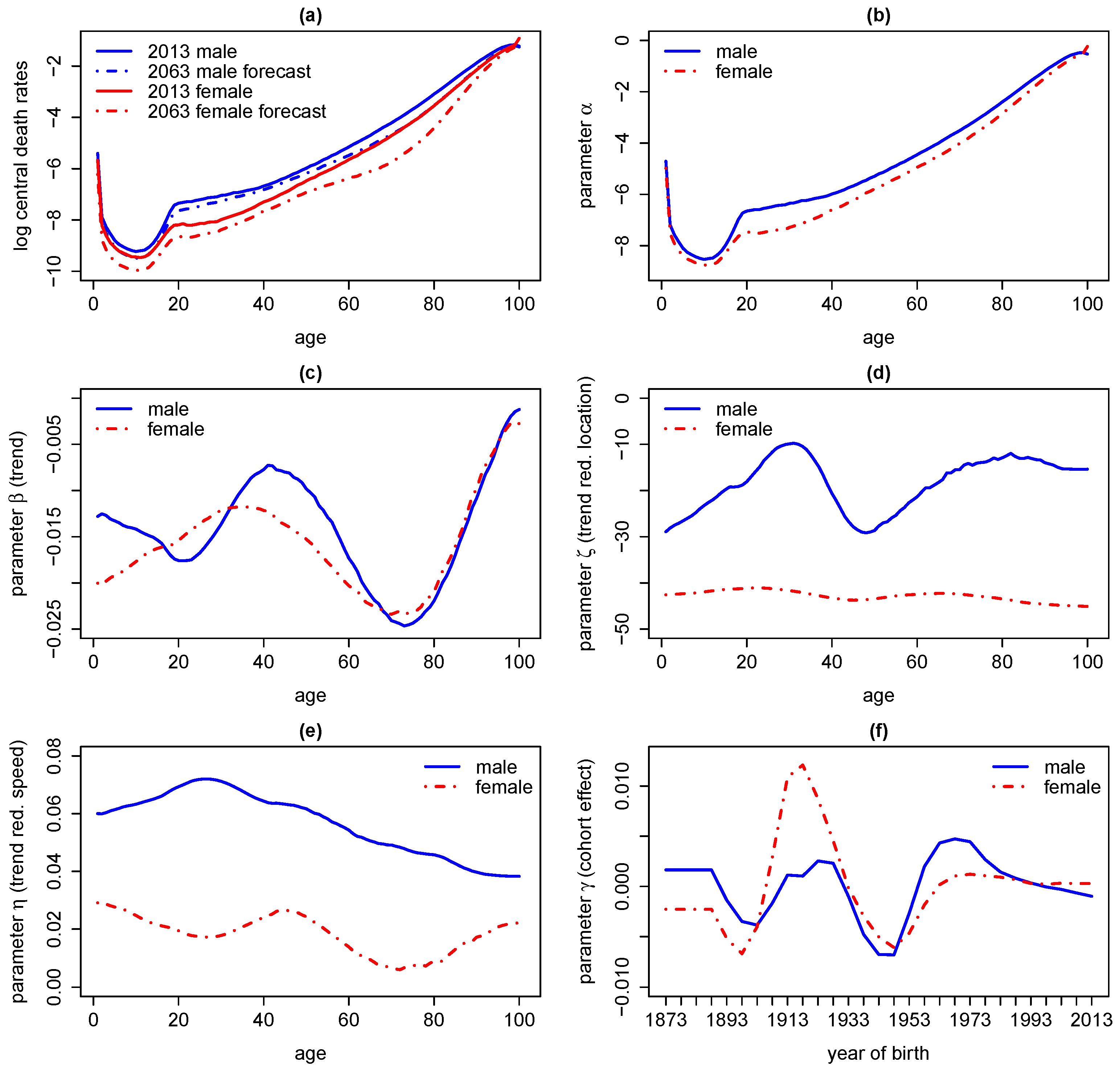
4.2. Forecasting Death Probabilities

Forecasting death probabilities and central death rates within our proposed model is straight forward using Equation (3). In the special case with just idiosyncratic risk, i.e., $K=0$, death indicators can be assumed to be Bernoulli distributed instead of being Poisson distributed in which case we may write the likelihood function in the form

$${\ell }^{\mathrm{B}}(\widehat{N}|\alpha ,\beta ,\zeta ,\eta ,\gamma )=\prod _{t=1}^T\prod _{a=0}^A\prod _{g\in \{\mathrm{f},\mathrm{m}\}}\left(\genfrac{}{}{0pt}{}{E_{a,g}\left(t\right)}{{\widehat{N}}_{a,g,0}\left(t\right)}\right)m_{a,g}{\left(t\right)}^{{\widehat{N}}_{a,g,0}\left(t\right)}{(1-m_{a,g}\left(t\right))}^{E_{a,g}\left(t\right)-{\widehat{N}}_{a,g,0}\left(t\right)},$$

with $0\le {\widehat{N}}_{a,g,0}\left(t\right)\le E_{a,g}\left(t\right)$. Due to possible overfitting, derived estimates may not be sufficiently smooth across age categories $a\in \{0,\cdots ,A\}$. Therefore, if we switch to a Bayesian setting, we may use regularisation via prior distributions to obtain stabler results. To guarantee smooth results and a sufficient stochastic foundation, we suggest the usage of Gaussian priors with mean zero and a specific correlation structure, i.e., $\pi (\alpha ,\beta ,\zeta ,\eta ,\gamma )=\pi \left(\alpha \right)\pi \left(\beta \right)\pi \left(\zeta \right)\pi \left(\eta \right)\pi \left(\gamma \right)$ with

$$log\pi \left(\alpha \right):=-c_{\alpha }\sum _{g\in \{\mathrm{f},\mathrm{m}\}}\left(\sum _{a=0}^{A-1}{({\alpha }_{a,g}-{\alpha }_{a+1,g})}^2+{\epsilon }_{\alpha }\sum _{a=0}^A{\alpha }_{a,g}^2\right)+log\left(d_{\alpha }\right),c_{\alpha },d_{\alpha },{\epsilon }_{\alpha }>0,$$

(13)

and correspondingly for $\beta$, $\zeta$, $\eta$ and $\gamma$. Parameters $c_{\alpha }$ (correspondingly for $\beta$, $\zeta$, $\eta$ and $\gamma$) is a scaling parameters and directly associated with the variance of Gaussian priors while normalisation-parameter $d_{\alpha }$ guarantees that $\pi \left(\alpha \right)$ is a proper Gaussian density. Penalty-parameter ${\epsilon }_{\alpha }$ scales the correlation amongst neighbour parameters in the sense that the lower it gets, the higher the correlation. The more we increase $c_{\alpha }$ the stronger the influence of, or the believe in the prior distribution. This particular prior density penalises deviations from the ordinate which is a mild conceptual shortcoming as this does not accurately reflect our prior believes. Setting ${\epsilon }_{\alpha }=0$ gives an improper prior with uniformly distributed (on $\mathbb{R}$) marginals such that we gain that there is no prior believe in expectations of parameters but, simultaneously, lose the presence of variance-covariance-matrices and asymptotically get perfect positive correlation across parameters of different ages. Still, whilst lacking theoretical properties, better fits to data are obtained by setting ${\epsilon }_{\alpha }=0$. For example, setting ${\epsilon }_{\alpha }={\epsilon }_{\beta }={10}^{-2}$ and ${\epsilon }_{\zeta }={\epsilon }_{\eta }={\epsilon }_{\gamma }={10}^{-4}$ yields a prior correlation structure which decreases with higher age differences and which is always positive as given in subfigure (a) of Figure 2.

There exist many other reasonable choices for Gaussian prior densities. For example, replacing graduation terms ${({\alpha }_{a,g}-{\alpha }_{a+1,g})}^2$ in Equation (13) by higher order differences of the form ${\left({\sum }_{\nu =0}^k{(-1)}^{\nu }\left(\genfrac{}{}{0pt}{}{k}{\nu }\right){\alpha }_{a,g+\nu }\right)}^2$ yields a penalisation for deviations from a straight line with $k=2$, see subfigure (b) in Figure 2, or from a parabola with $k=3$, see subfigure (c) in Figure 2. The usage of higher order differences for graduation of statistical estimates goes back to the Whittaker–Henderson method. Taking $k=2,3$ unfortunately yields negative prior correlations amongst certain parameters which is why we do not recommend their use. Of course, there exist many further possible choices for prior distributions. However, in our example, we set ${\epsilon }_{\alpha }={\epsilon }_{\beta }={\epsilon }_{\zeta }={\epsilon }_{\eta }={\epsilon }_{\gamma }=0$ as this yields accurate results whilst still being reasonably smooth.

An optimal choice of regularisation parameters $c_{\alpha },c_{\beta },c_{\zeta },c_{\eta }$ and $c_{\gamma }$ can be obtained by cross-validation.

Results for Australian data from 1971 to 2013 with $t_0=2013$ are given in Figure 3. Using MCMC we derive estimates for logarithmic central death rates $log{m}_{a,g}\left(t\right)$ with corresponding forecasts, mortality trends ${\beta }_{a,g}$, as well as trend reduction parameters ${\zeta }_{a,g},{\eta }_{a,g}$ and cohort effects ${\gamma }_{a-t}$. As we do not assume common stochastic risk factors, the MCMC algorithm we use can be implemented very efficiently such that $40000$ samples from the posterior distribution of all parameters are derived within a minute. We observe negligible parameter uncertainty due to a long period of data. Further, regularisation parameters obtained by cross-validation are given by $c_{\alpha }=500$, $c_{\beta }=c_{\eta }=30,000c_{\alpha }$, $c_{\zeta }=c_{\alpha }/20$ and $c_{\gamma }=1000c_{\alpha }$.

We can draw some immediate conclusions. Firstly, we see an overall improvement in mortality over all ages where the trend is particularly strong for young ages and ages between 60 and 80 whereas the trend vanishes towards the age of 100, maybe implying a natural barrier for life expectancy. Due to sparse data the latter conclusion should be treated with the utmost caution. Furthermore, we see the classical hump of increased mortality driven by accidents around the age of 20 which is more developed for males.

Secondly, estimates for ${\zeta }_{a,g}$ suggest that trend acceleration switched to trend reduction throughout the past 10 to 30 years for males while for females this transition already took place 45 years ago. However, note that parameter uncertainty (under MCMC) associated with ${\zeta }_{a,g}$ is high, particularly if estimates are not regularised. Estimates for ${\eta }_{a,g}$ show that the speed of trend reduction is much stronger for males than for females. Estimates for ${\gamma }_{a-t}$ show that the cohort effect is particularly strong (in the sense of increased mortality) for the generation born between 1915 and 1930 (probably associated with World War II) and particularly weak for the generation born around 1945. However, considering cohort effects makes estimation and forecasts significantly less stable for the used data, which is why we recommend to set ${\gamma }_{a-t}=0$.

Based on forecasts for death probabilities, expected future life time can be estimated. To be consistent concerning longevity risk, mortality trends have to be included as a 60-year-old today will probably not have as good medication as a 60-year-old in several decades. However, it seems that this is not the standard approach in the literature. Based on the definitions above, expected (curtate) future life time of a person at date T is given by $e_{a,g}\left(T\right)=\mathbb{E}\left[K_{a,g}\left(T\right)\right]={\sum }_{k=1}^{\infty }{}_k{p}_{a,g}\left(T\right)$, where survival probabilities over $k\in \mathbb{N}$ years are given by ${}_k{p}_{a,g}\left(T\right):={\prod }_{j=0}^{k-1}\left(1-q_{a+j,g}(T+j)\right)$ and where $K_{a,g}\left(T\right)$ denotes the number of completed future years lived by a person of particular age and gender at time T. Approximating death probabilities by central death rates, for newborns in Australia we get a life expectancy of roughly 83 years for males and $89.5$ for females born in 2013, see

Table 4. Curtate future life time $e_{a,g}\left(T\right)$ for males and females in 2013.

Age in 2013	0 (Newborn)	20	40	60	80
male	$83.07$	$63.33$	$43.62$	$24.44$	$8.26$
female	$89.45$	$69.05$	$48.20$	$27.76$	$9.88$

. Thus, comparing these numbers to a press release from October 2014 from the Australian Bureau of Statistics5 saying that ‘Aussie men now expected to live past 80’ and ‘improvements in expected lifespan for women has since slowed down, increasing by around four years over the period—it’s 84.3 now’, our results show a much higher life expectancy due to the consideration of mortality trends.

5. A Link to the Extended CreditRisk${}^{+}$ Model and Applications

5.1. The ECRP Model

In this section we establish the connection from our proposed stochastic mortality model to the risk aggregation model extended CreditRisk${}^{+}$ (abbreviated as ECRP), as given in (Schmock 2017, section 6).

Definition 7 (Policyholders and number of deaths).

Let $\{1,\cdots ,E\}$ with $E\in \mathbb{N}$ denote the set of people (termed as policyholders in light of insurance applications) in the portfolio and let random variables $N_1,\cdots ,N_E:\Omega \to {\mathbb{N}}_0$ indicate the number of deaths of each policyholder in the following period. The event $\{N_i=0\}$ indicates survival of person i whilst $\{N_i\ge 1\}$ indicates death.

Definition 8 (Portfolio quantities).

Given Definition 7, the independent random vectors $Y_1,\cdots ,Y_E:\Omega \to {\mathbb{N}}_0^d$ with $d\ge 1$ dimensions denote portfolio quantities within the following period given deaths of policyholders, i.e., on $\{N_i\ge 1\}$ for all $i\in \{1,\cdots ,E\}$, and are independent of $N_1,\cdots ,N_E$.

Remark 5.

(Portfolio quantities).

(a) 

For applications in the context of internal models we may set $Y_i$ as the best estimate liability, i.e., discounted future cash flows, of policyholder i at the end of the period. Thus, when using stochastic discount factors or contracts with optionality, for example, portfolio quantities may be stochastic.

(b) 

In the context of portfolio payment analysis we may set $Y_i$ as the payments (such as annuities) to i over the next period. We may include premiums in a second dimension in order to get joint distributions of premiums and payments.

(c) 

For applications in the context of mortality estimation and projection we set $Y_i=1$.

(d) 

Using discretisation which preserves expectations (termed as stochastic rounding in (Schmock 2017, section 6.2.2), we may assume $Y_i$ to be ${[0,\infty )}^d$-valued .

Definition 9 (Aggregated portfolio quantities).

Given Definitions 7 and 8, aggregated portfolio quantities due to deaths are given by

$$S:=\sum _{i=1}^E\sum _{j=1}^{N_i}{Y}_{i,j},$$

where ${\left(Y_{i,j}\right)}_{j\in \mathbb{N}}$ for every $i\in \{1,\cdots ,E\}$ is an i.i.d. sequence of random variables with the same distributions as $Y_i$.

Remark 6.

In the context of term life insurance contracts, for example, S is the sum of best estimates of payments and premiums which are paid and received, respectively, due to deaths of policyholders, see Section 5.2. In the context of annuities, S is the sum of best estimates of payments and premiums which need not be paid and are received, respectively, due to deaths of policyholders. Then, small values of S, i.e., the left tail of its distribution, is the part of major interest and major risk.

It is a demanding question how to choose the modelling setup such that the distribution of S can be derived efficiently and accurately. Assuming $N_i$ to be Bernoulli distributed is not suitable for our intended applications as computational complexity explodes. Therefore, to make the modelling setup applicable in practical situations and to ensure a flexible handling in terms of multi-level dependence, we introduce the ECRP model which is based on extended CreditRisk${}^{+}$, see (Schmock 2017, section 6).

Definition 10 (The ECRP model).

Given Definitions 7 and 8, the ECRP model satisfies the following additional assumptions:

(a) 

Consider independent random common risk factors ${\Lambda }_1,\cdots ,{\Lambda }_K:\Omega \to [0,\infty )$ which have a gamma distribution with mean $e_k=1$ and variance ${\sigma }_k^2>0$, i.e., with shape and inverse scale parameter ${\sigma }_k^{-2}$. Also the degenerate case with ${\sigma }_k^2=0$ for $k\in \{1,\cdots ,K\}$ is allowed. Corresponding weights $w_{i,0},\cdots ,w_{i,K}\in [0,1]$ for every policyholder $i\in \{1,\cdots ,E\}$. Risk index zero represents idiosyncratic risk and we require $w_{i,0}+\cdots +w_{i,K}=1$.

(b) 

Deaths $N_{1,0},\cdots ,N_{E,0}:\Omega \to {\mathbb{N}}_0$ are independent from one another, as well as all other random variables and, for all $i\in \{1,\cdots ,E\}$, they are Poisson distributed with intensity $m_i{w}_{i,0}$, i.e.,

$$\mathbb{P}\left(\bigcap _{i=1}^E\{N_{i,0}={\widehat{N}}_{i,0}\}\right)=\prod _{i=1}^E{e}^{-m_i{w}_{i,0}}\frac{{\left(m_i{w}_{i,0}\right)}^{{\widehat{N}}_{i,0}}}{{\widehat{N}}_{i,0}!},{\widehat{N}}_{1,0},\cdots ,{\widehat{N}}_{E,0}\in {\mathbb{N}}_0.$$

(c) 

Given risk factors, deaths ${\left(N_{i,k}\right)}_{i\in \{1,\cdots ,E\},k\in \{1,\cdots ,K\}}:\Omega \to {\mathbb{N}}_0^{E\times K}$ are independent and, for every policyholder $i\in \{1,\cdots ,E\}$ and $k\in \{1,\cdots ,K\}$, they are Poisson distributed with random intensity $m_i{w}_{i,k}{\Lambda }_k$, i.e.,

$$\mathbb{P}\left(\bigcap _{i=1}^E\bigcap _{k=1}^K\{N_{i,k}={\widehat{N}}_{i,k}\}|{\Lambda }_1,\cdots ,{\Lambda }_K\right)=\prod _{i=1}^E\prod _{k=1}^K{e}^{-m_i{w}_{i,k}{\Lambda }_k}\frac{{\left(m_i{w}_{i,k}{\Lambda }_k\right)}^{{\widehat{N}}_{i,k}}}{{\widehat{N}}_{i,k}!}\mathrm{a}.\mathrm{s}.,$$

for all $n_{i,k}\in {\mathbb{N}}_0$.

(d) 

For every policyholder $i\in \{1,\cdots ,E\}$, the total number of deaths $N_i$ is split up additively according to risk factors as $N_i=N_{i,0}+\cdots +N_{i,K}$. Thus, by model construction, $\mathbb{E}\left[N_i\right]=m_i(w_{i,0}+\cdots +w_{i,K})=m_i$.

Given Definition 7, central death rates are given by $m_i=\mathbb{E}\left[N_i\right]$ and death probabilities, under piecewise constant death rates, are given by $q_i=1-exp(-m_i)$.

Remark 7.

Assuming that central death rates and weights are equal for all policyholders for the same age and gender, it is obvious that the ECRP corresponds one-to-one to our proposed stochastic mortality model, as given in Definition 1, if risk factors are independent gamma distributed.

In reality, number of deaths are Bernoulli random variables as each person can just die once. Unfortunately in practice, such an approach is not tractable for calculating P&L distributions of large portfolios as execution times explode if numerical errors should be small. Instead, we will assume the number of deaths of each policyholder to be compound Poisson distributed. However, for estimation of life tables we will assume the number of deaths to be Bernoulli distributed. Poisson distributed deaths give an efficient way for calculating P&L distributions using an algorithm based on Panjer’s recursion, also for large portfolios, see (Schmock 2017, section 6.7). The algorithm is basically due to Giese (2003) for which Haaf et al. (2004) proved numerical stability. The relation to Panjer’s recursion was first pointed out in (Gerhold et al. 2010, section 5.5). Schmock (2017) in section 5.1 generalised the algorithm to the multivariate case with dependent risk factors and risk groups, based on the multivariate extension of Panjer’s algorithm given by Sundt (1999). The algorithm is numerically stable since just positive terms are added up. To avoid long execution times for implementations of extended CreditRisk${}^{+}$ with large annuity portfolios, greater loss units and stochastic rounding, see (Schmock 2017, section 6.2.2), can be used.

However, the proposed model allows for multiple (Poisson) deaths of each policyholder and thus approximates the ‘real world’ with single (Bernoulli) deaths. From a theoretical point of view, this is justified by the Poisson approximation and generalisations of it, see for example Vellaisamy and Chaudhuri (1996). Since annual death probabilities for ages up to 85 are less than 10%, multiple deaths are relatively unlikely for all major ages. However, implementations of this algorithm are significantly faster than Monte Carlo approximations for comparable error (Poisson against Bernoulli) levels.

As an illustration we take a portfolio with $E=\mathrm{10,000}$ policyholders having central death rate $m:=m_i=0.05$ and payments $Y_i=1$. We then derive the distribution of S using the ECRP model for the case with just idiosyncratic risk, i.e., $w_{i,0}=1$ and Poisson distributed deaths, and for the case with just one common stochastic risk factor ${\Lambda }_1$ with variance ${\sigma }_1=0.1$ and no idiosyncratic risk, i.e., $w_{i,1}=1$ with mixed Poisson distributed deaths. Then, using $\mathrm{50,000}$ simulations of the corresponding model where $N_i$ is Bernoulli distributed or mixed Bernoulli distributed given truncated risk factor ${\Lambda }_1|{\Lambda }_1\le \frac{1}{m}$, we compare the results of the ECRP model to Monte Carlo, respectively. Truncation of risk factors in the Bernoulli model is necessary as otherwise death probabilities may exceed one. We observe that the ECRP model drastically reduces execution times in ‘R’ at comparable error levels and leads to a speed up by the factor of 1000. Error levels in the purely idiosyncratic case are measured in terms of total variation distance between approximations and the binomial distribution with parameters $(\mathrm{10,000},0.05)$ which arises as the independent sum of all Bernoulli random variables. Error levels in the purely non-idiosyncratic case are measured in terms of total variation distance between approximations and the mixed binomial distribution where for the ECRP model we use Poisson approximation to get an upper bound. the total variation between those distributions is $0.0159$ in our simulation and, thus, dominates the Poisson approximation in terms of total variation. Results are summarised in

Table 5. Quantiles, execution times (speed) and total variation distance (accuracy) of Monte Carlo with Bernoulli deaths and $\mathrm{50,000}$ simulations, as well as the extended CreditRisk${}^{+}$ (ECRP) model with Poisson deaths, given a simple portfolio.

	Quantiles					Speed	Accuracy
1%	10%	50%	90%	99%
Bernoulli (MC), $w_{i,0}=1$	450	472	500	528	552	$22.99$ s	$0.0187$
Poisson (ECRP), $w_{i,0}=1$	449	471	500	529	553	$0.01$ s	$0.0125$
Bernoulli (MC), $w_{i,1}=1$	202	310	483	711	936	$23.07$ s	$0.0489$
Poisson (ECRP), $w_{i,1}=1$	204	309	483	712	944	$0.02$ s	≤0.0500

.

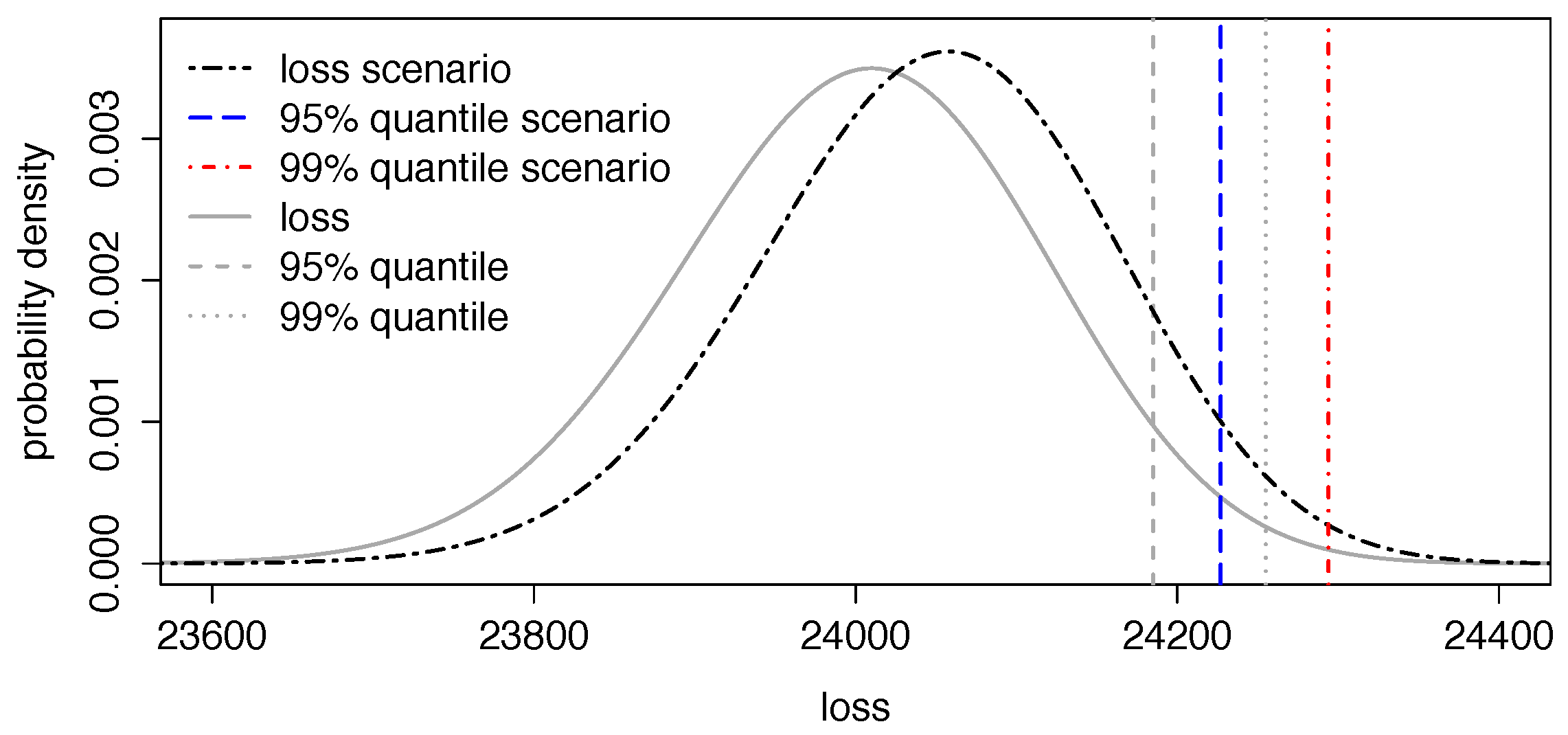
5.2. Application I: Mortality Risk, Longevity Risk and Solvency II Application

In light of the previous section, life tables can be projected into the future and, thus, it is straightforward to derive best estimate liabilities (BEL) of annuities and life insurance contracts. The possibility that death probabilities differ from an expected curve, i.e., estimated parameters do no longer reflect the best estimate and have to be changed, contributes to mortality or longevity risk, when risk is measured over a one year time horizon as in Solvency II and the duration of in-force insurance contracts exceeds this time horizon. In our model, this risk can be captured by considering various MCMC samples ${({\widehat{\theta }}^h)}_{h=1,\cdots ,m}$ (indexed by superscript h) of parameters $\theta =(\alpha ,\beta ,\zeta ,\eta ,\gamma )$ for death probabilities, yielding distributions of BELs. For example, taking $D(T,T+t)$ as the discount curve from time $T+t$ back to T and choosing an MCMC sample ${\widehat{\theta }}^h$ of parameters to calculate death probabilities $q_{a,g}^h\left(T\right)$ and survival probabilities $p_{a,g}^h\left(T\right)$ at age a with gender g, the BEL for a term life insurance contract which pays 1 unit at the end of the year of death within the contract term of d years is given by

$$A_{a,g}^T\left({\widehat{\theta }}^h\right)=D(T,T+1)q_{a,g}^h\left(T\right)+\sum _{t=1}^{d}D(T,T+t+1)·{}_t{p}_{a,g}^h\left(T\right)q_{a+t,g}^h(T+t).$$

(14)

In a next step, this approach can be used as a building block for (partial) internal models to calculate basic solvency capital requirements (BSCR) for biometric underwriting risk under Solvency II, as illustrated in the following example.

Consider an insurance portfolio at time 0 with $E\in \mathbb{N}$ whole life insurance policies with lump sum payments $C_i>0$, for $i=1,\cdots ,E$, upon death at the end of the year. Assume that all assets are invested in an EU government bond (risk free under the standard model of the Solvency II directive) with maturity 1, nominal $A_0$ and coupon rate $c>-1$. Furthermore, assume that we are only considering mortality risk and ignore profit sharing, lapse, costs, reinsurance, deferred taxes, other assets and other liabilities, as well as the risk margin. Note that in this case, basic own funds, denoted by ${\mathrm{BOF}}_t$, are given by market value of assets minus BEL at time t, respectively. Then, the BSCR at time 0 is given by the 99.5% quantile of the change in basic own funds over the period $[0,1]$, denoted by $\Delta {\mathrm{BOF}}_1$, which can be derived by, see Equation (14),

$$\begin{array}{cc}\hfill \Delta {\mathrm{BOF}}_1& ={\mathrm{BOF}}_0-D(0,1){\mathrm{BOF}}_1=A_0\left(1-D(0,1)(1+c)\right)-\sum _{i=1}^E{C}_i{A}_{a,g}^0\left(\widehat{\theta }\right)\hfill \\ & +\frac{D(0,1)}{m}\sum _{h=1}^m\left(\sum _{i=1}^E{C}_i{A}_{a+1,g}^1\left({\widehat{\theta }}^h\right)+\sum _{i=1}^E\sum _{j=1}^{N_i^h}{C}_i\left(1-A_{a+1,g}^1\left({\widehat{\theta }}^h\right)\right)\right).\hfill \end{array}$$

(15)

where $\widehat{\theta }:=\frac{1}{m}{\sum }_{h=1}^m{\widehat{\theta }}^h$ and where $N_1^h,\cdots ,N_E^h$ are independent and Poisson distributed with $\mathbb{E}\left[N_i^h\right]=q_{a_i,g_i}^h\left(0\right)$ with policyholder i belonging to age group $a_i$ and of gender $g_i$. The distribution of the last sum above can be derived efficiently by Panjer recursion. This example does not require a consideration of market risk and it nicely illustrates how mortality risk splits into a part associated with statistical fluctuation (experience variance: Panjer recursion) and into a part with long-term impact (change in assumptions: MCMC). Note that by mixing $N_i$ with common stochastic risk factors, we may include other biometric risks such as morbidity.

Consider a portfolio with 100 males and females at each age between 20 and 60 years, each having a 40-year term life insurance, issued in 2014, which provides a lump sum payment between 10,000 and 200,000 (randomly chosen for each policyholder) if death occurs within these 40 years. Using MCMC samples and estimates based on the Austrian data from 1965 to 2014 as given in the previous section, we may derive the change in basic own funds from 2014 to 2015 by Equation (15) using the extended CreditRisk${}^{+}$ algorithm. The 99.5% quantile of change in BOFs, i.e., the SCR, is lying slightly above one million. If we did not consider parameter risk in the form of MCMC samples, the SCR would decrease by roughly 33%.

5.3. Application II: Impact of Certain Health Scenarios in Portfolios

Analysis of certain health scenarios and their impact on portfolio P&L distributions is straightforward As an explanatory example, assume $m=1600$ policyholders which distribute uniformly over all age categories and genders, i.e., each age category contains 100 policyholders with corresponding death probabilities, as well as weights as previously estimated and forecasted for 2012. Annuities $Y_i$ for all $i\in \{1,\cdots ,E\}$ are paid annually and take deterministic values in $\{11,\cdots ,20\}$ such that ten policyholders in each age and gender category share equally high payments. We now analyse the effect on the total amount of annuity payments in the next period under the scenario, indexed by ‘scen’, that deaths due to neoplasms are reduced by 25% in 2012 over all ages. In that case, we can estimate the realisation of risk factor for neoplasms, see Equation (7), which takes an estimated value of $0.7991$. Running the ECRP model with this risk factor realisation being fixed, we end up with a loss distribution $L^{\mathrm{scen}}$ where deaths due to neoplasms have decreased. Figure 4 then shows probability distributions of traditional loss L without scenario, as well as of scenario loss $L^{\mathrm{neo}}$ with corresponding 95% and 99% quantiles. We observe that a reduction of 25% in cancer crude death rates leads to a remarkable shift in quantiles of the loss distribution as fewer people die and, thus, more annuity payments have to be made.

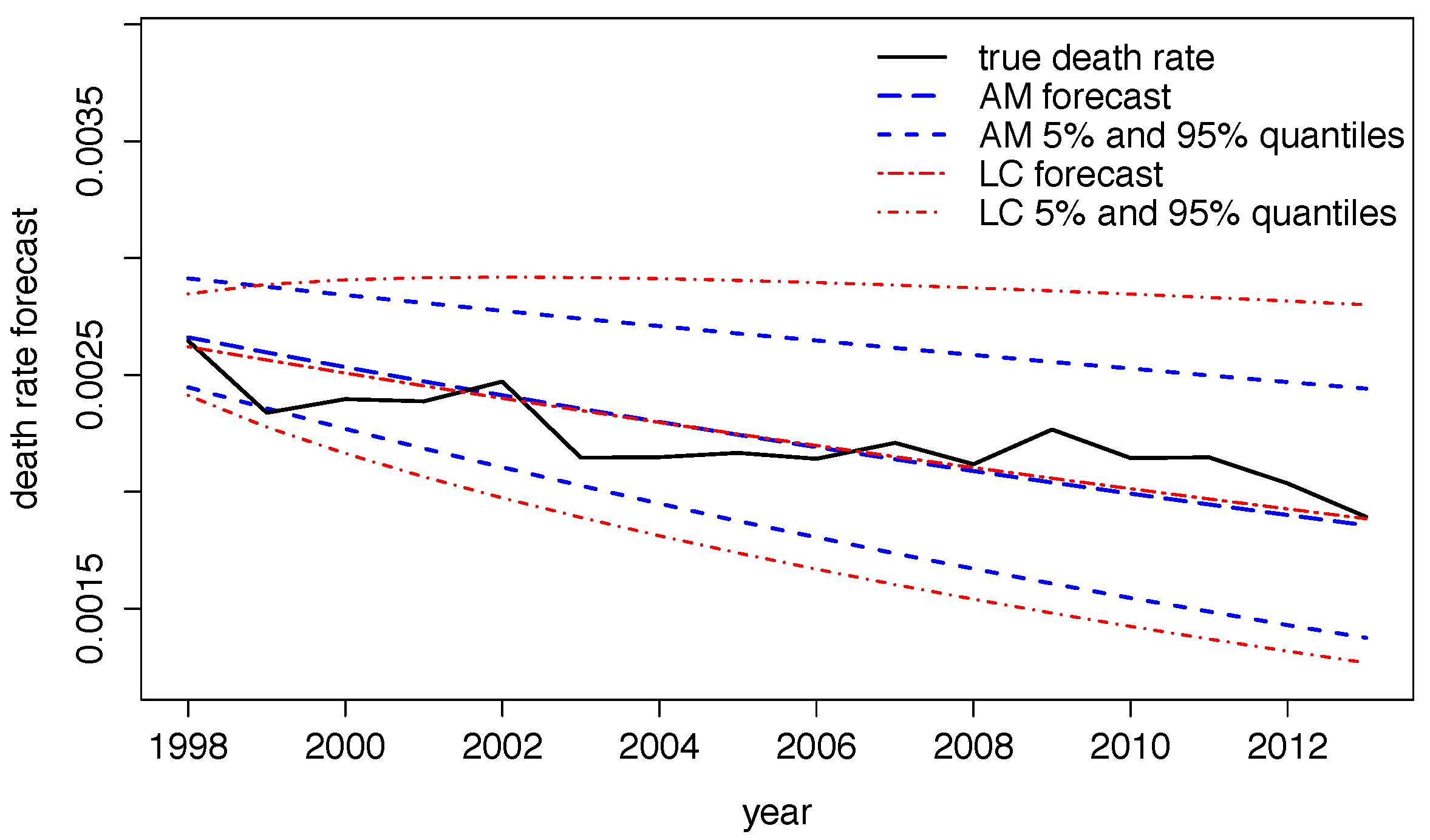
5.4. Application III: Forecasting Central Death Rates and Comparison With the Lee–Carter Model

We can compare out-of-sample forecasts of death rates from our proposed model to forecasts obtained by other mortality models. Here, we choose the traditional Lee–Carter model as a proxy as our proposed model is conceptionally based on a similar idea. We make the simplifying assumption of a constant population for out-of-sample time points.

Using the ECRP model it is straight-forward to forecast central death rates and to give corresponding confidence intervals via setting $Y_j\left(t\right):=1$. Then, for an estimate $\widehat{\theta }$ of parameter vector $\theta$ run the ECRP model with parameters forecasted, see Equations (3) and (4). We then obtain the distribution of the total number of deaths $S_{a,g}\left(t\right)$ given $\widehat{\theta }$ and, thus, forecasted death rate ${\widehat{m}}_{a,g}\left(t\right)$ is given by $\mathbb{P}\left({\widehat{m}}_{a,g}\left(t\right)=N/E_{a,g}\left(T\right)\right)=\mathbb{P}(S_{a,g}\left(t\right)=N)$, for all $N\in {\mathbb{N}}_0$.

Uncertainty in the form of confidence intervals represent statistical fluctuations, as well as random changes in risk factors. Additionally, using results obtained by Markov chain Monte Carlo (MCMC) it is even possible to incorporate parameter uncertainty into predictions. To account for an increase in uncertainty for forecasts we suggest to assume increasing risk factor variances for forecasts, e.g., ${\tilde{\sigma }}_k^2\left(t\right)={\sigma }_k^2{(1+d(t-T))}^2$ with $d\ge 0$. A motivation for this approach with $k=1$ is the following: A major source of uncertainty for forecasts lies in an unexpected deviation from the estimated trend for death probabilities. We may therefore assume that rather than being deterministic, forecasted values $m_{a,g}\left(t\right)$ are beta distributed (now denoted by $M_{a,g}\left(t\right)$) with $\mathbb{E}\left[M_{a,g}\left(t\right)\right]=m_{a,g}\left(t\right)$ and variance ${\sigma }_{a,g}^2\left(t\right)$ which is increasing in time. Then, given independence amongst risk factor ${\Lambda }_1$ and $M_{a,g}\left(t\right)$, we may assume that there exists a future point in time $t_0$ such that

$${\sigma }_{a,g}^2\left(t_0\right)=\frac{m_{a,g}\left(t_0\right)(1-m_{a,g}\left(t_0\right))}{{\sigma }_1^{-2}+1}.$$

In that case, $M_{a,g}\left(t_0\right){\Lambda }_1$ is again gamma distributed with mean one and increased variance $m_{a,g}\left(t_0\right){\sigma }_1^2$ (instead of $m_{a,g}^2\left(t_0\right){\sigma }_1^2$ for the deterministic case). Henceforth, it seems reasonable to stay within the family of gamma distributions for forecasts and just adapt variances over time. Of course, families for these variances for gamma distributions can be changed arbitrarily and may be selected via classical information criteria.

Using in-sample data, d can be estimated via Equation (5) with all other parameters being fixed. Using Australian death and population data for the years 1963 to 1997 we estimate model parameters via MCMC in the ECRP model with one common stochastic risk factor having constant weight one. In average, i.e., for various forecasting periods and starting at different dates, parameter d takes the value $0.22$ in our example. Using fixed trend parameters as above, and using the mean of 30,000 MCMC samples, we forecast death rates and corresponding confidence intervals out of sample for the period 1998 to 2013. We can then compare these results to crude death rates within the stated period and to forecasts obtained by the Lee–Carter model which is shown in Figure 5 for females aged 50 to 54 years. We observe that crude death rates mostly fall in the 90% confidence band for both procedures. Moreover, Lee–Carter forecasts lead to wider spreads of quantiles in the future whilst the ECRP model suggests a more moderate increase in uncertainty. Taking various parameter samples from the MCMC chain and deriving quantiles for death rates, we can extract contributions of parameter uncertainty in the ECRP model coming from posterior distributions of parameters.

Within our approach to forecast death rates, it is now possible to derive contributions of various sources of risk. If we set $\delta =0$ we get forecasts where uncertainty solely comes from statistical fluctuations and random changes in risk factors. Using $\delta =0.22$ this adds the uncertainty increase associated with uncertainty for forecasts. Finally, considering several MCMC samples this adds parameter risk. We observe that the contribution of statistical fluctuations and random changes in risk factors decreases from 63% in 1998 to 20% in 2013. Adding the increase in uncertainty for forecasts gives a roughly constant contribution of 72% which implies that $\delta$ becomes the main driver of risk in the long term. On top of that, parameter uncertainty leaves a constant contribution of 28%.

5.5. Considered Risks

Regulators often require security margins in life tables when modelling annuity or certain life insurance products and portfolios to account for different sources of risk, including trends, volatility risk, model risk and parameter risk, Kainhofer et al. (2006) as well as Pasdika and Wolff (2005).

In the ECRP model, mortality trends are incorporated via families for death probabilities which are motivated by the Lee–Carter model. It is straight forward to arbitrarily change parameter families such that it fits the data as in the case when trends change fundamentally. If other families for weights are used, one always has to check that they sum up to one over all death causes. Note that for certain alternative parameter families, mean estimates obtained from Markov chain Monte Carlo do not necessarily sum up to one anymore. Changing model parameter families may also be necessary when using long-term projections since long-term trends are fundamentally different from short-term trends. Further estimation and testing procedures for trends in composite Poisson models in the context of convertible bonds can be found in Schmock (1999). Trends for weights are particularly interesting insofar as the model becomes sensitive to the change in the vulnerability of policyholders to different death causes over time. Cross dependencies over different death causes and different ages can occur. Such an effect can arise as a reduction in deaths of a particular cause can lead to more deaths in another cause, several periods later, as people have to die at some point. Furthermore, the ECRP model captures unexpected, temporary deviations from a trend with the variability introduced by common stochastic risk factors which effect all policyholders according to weights simultaneously.

Assuming that the model choice is right and that estimated values are correct, life tables still just give mean values of death probabilities over a whole population. Therefore, in the case of German data it is suggested to add a non gender specific due to legal reasons and it is set to 7.4% to account for the risk of random fluctuations in deaths, approximately at a 95% quantile, see German Actuarial Association (DAV) (Todesfallrisiko 2009, section 4.1). In the ECRP model this risk is captured automatically by risk aggregation. As a reference to the suggested security margin of $7.4$% on death probabilities, we can use the same approach as given in Section 5.4 to estimate quantiles for death rates via setting $Y_j=1$. These quantiles then correspond to statistical fluctuations around death probabilities. We roughly observe an average deviation from death probability of 8.4% for the 5% quantile and of 8.7% for the 95% quantile of females aged 55 to 60 years in 2002, i.e., these values are in line with a security margin of 7.4%.

The risk of wrong parameter estimates, i.e., that realised death probabilities deviate from estimated values, can be captured using MCMC as described in Section 3.3 where we sample from the joint posterior distributions of the estimators. As our proposed extended CreditRisk${}^{+}$ algorithm is numerically very efficient, we can easily run the ECRP model for several thousand samples from the MCMC chain to derive sensitivities of quantiles, for example. Note that parameter risk is closely linked to longevity risk. To cover the risk of fundamental changes in future death probabilities, Section 5.4 provides an approach where future risk factor variances increase over time.

Modelling is usually a projection of a sophisticated real world problem on a relatively simple subspace which cannot cover all facets and observations in the data. Therefore, when applying the ECRP model to a portfolio of policyholders, we usually find structural differences to the data which is used for estimation. There may also be a difference in mortality rates between individual companies or between portfolios within a company since different types of insurance products attract different types of policyholders with a different individual risk profile. In Germany, for these risks a minimal security margin of ten% is suggested, see (Pasdika and Wolff 2005, section 2.4.2). Within the ECRP model, this risk can be addressed by using individual portfolio data instead of the whole population. Estimates from the whole population or a different portfolio can be used as prior distributions under MCMC which, in case of sparse data, makes estimation more stable. Another possibility for introducing dependency amongst two portfolios is the introduction of a joint stochastic risk factor for both portfolios. In that case, estimation can be performed jointly with all remaining (except risk factors and their variances) parameters being individually estimated for both portfolios. In contrast to the whole population, observed mortality rates in insurance portfolios often show a completely different structure due to self-selection of policyholders. In particular, for ages around 60, this effect is very strong. In Germany, a security margin for death probabilities of 15% is suggested to cover selection effects, see DAV (Todesfallrisiko 2009, section 4.2). In the literature, this effect is also referred to as basis risk, Li and Hardy (2011). As already mentioned, instead of using a fixed security margin, this issue can be tackled by using portfolio data with estimates from the whole population serving as prior distribution. Again, dependence amongst a portfolio and the whole population can be introduced by a joint stochastic risk factor in the ECRP model.

Alternatively, in (Kainhofer et al. 2006, section 4.7.1) it is suggested that all these risks are addressed by adding a constant security margin on the trend. This approach has the great conceptional advantage that the security margin is increasing over time and does not diminish as in the case of direct security margins on death probabilities.

5.6. Generalised and Alternative Models

Up to now, we applied a simplified version of extended CreditRisk${}^{+}$ to derive cumulative payments in annuity portfolios. A major shortcoming in this approach is the limited possibility of modelling dependencies amongst policyholders and death causes. In the most general form of extended CreditRisk${}^{+}$ as described in (Schmock 2017, section 6), it is possible to introduce risk groups which enable us to model joint deaths of several policyholders and it is possible to model dependencies amongst death causes. Dependencies can take a linear dependence structure combined with dependence scenarios to model negative correlations as well. Risk factors may then be identified with statistical variates such as average blood pressure, average physical activity or the average of smoked cigarettes, etc., and not directly with death causes. Moreover, for each policyholder individually, the general model allows for losses which depend on the underlying cause of death. This gives scope to the possibility of modelling—possibly new—life insurance products with payoffs depending on the cause of death as, for example, in the case of accidental death benefits. Including all extensions mentioned above, a similar algorithm may still be applied to derive loss distributions, see (Schmock 2017, section 6.7).

Instead of using extended CreditRisk${}^{+}$ to model annuity portfolios, i.e., an approach based on Poisson mixtures, we can assume a similar Bernoulli mixture model. In such a Bernoulli mixture model, conditionally Poisson distributed deaths are simply replaced by conditionally Bernoulli distributed deaths. In general, explicit and efficient derivation of loss distributions in the case of Bernoulli mixture models is not possible anymore. Thus, in this case, one has to rely on other methods such as Monte Carlo. Estimation of model parameters works similarly as discussed in Section 3. Poisson approximation suggests that loss distributions derived from Bernoulli and Poisson mixture models are similar in terms of total variation distance if death probabilities are small.

6. Model Validation and Model Selection

In this section we propose several validation techniques in order to check whether the ECRP model fits the given data or not. Results for Australian data, see Section 4.1, strongly suggest that the proposed model is suitable. If any of the following validation approaches suggested misspecification in the model or if parameter estimation did not seem to be accurate, one possibility to tackle these problems would be to reduce risk factors.

6.1. Validation via Cross-Covariance

For the first procedure, we transform deaths $N_{a,g,k}\left(t\right)$ to $N_{a,g,k}^{\prime }\left(t\right)$, see Section 3.4, such that this sequence has constant expectation and can thus be assumed to be i.i.d. Then, sample variances of transformed death counts, cumulated across age and gender groups, can be compared to MCMC confidence bounds from the model. In the death-cause-example all observed sample variances of $N_k\left(t\right)$ lie within 5%- and 95%-quantiles.

6.2. Validation via Independence

Number of deaths for different death causes are independent within the ECRP model as independent risk factors are assumed. Thus, for all $a,a^{\prime }\in \{1,\cdots ,A\}$ and $g,g^{\prime }\in \{\mathrm{f},\mathrm{m}\}$, as well as $k,k^{\prime }\in \{0,\cdots ,K\}$ with $k\ne k^{\prime }$ and $t\in U$, we have $\mathrm{Cov}(N_{a,g,k}\left(t\right),N_{a^{\prime },g^{\prime },k^{\prime }}\left(t\right))=0$. Again, transform the data as above and subsequently normalise the transformed data, given $\mathrm{Var}\left(N_{a,g,k}^{\prime }\left(t\right)|{\Lambda }_k\left(t\right)\right)>0$ a.s., as follows:

$$N_{a,g,k}^{*}\left(t\right):=\frac{N_{a,g,k}^{\prime }\left(t\right)-\mathbb{E}\left[N_{a,g,k}^{\prime }\left(t\right)\right|{\Lambda }_k\left(t\right)]}{\sqrt{\mathrm{Var}\left(N_{a,g,k}^{\prime }\left(t\right)\right|{\Lambda }_k\left(t\right))}}=\frac{N_{a,g,k}^{\prime }\left(t\right)-E_{a,g}{m}_{a,g}{w}_{a,g,k}{\Lambda }_k\left(t\right)}{\sqrt{E_{a,g}{m}_{a,g}{w}_{a,g,k}{\Lambda }_k\left(t\right)}}.$$

Using the conditional central limit theorem as in Grzenda and Zieba (2008), we have $N_{a,g,k}^{*}\left(t\right)\to N(0,1)$ in distribution as $E_{a,g}\left(t\right)\to \infty$ where $N(0,1)$ denotes the standard normal distribution. Thus, normalised death counts $n_{a,g,k}^{*}\left(t\right)$ are given by

$$n_{a,g,k}^{*}\left(t\right)=\frac{n_{a,g,k}^{\prime }\left(t\right)-E_{a,g}{\widehat{m}}_{a,g}{\widehat{w}}_{a,g,k}{\widehat{\lambda }}_k\left(t\right)}{\sqrt{E_{a,g}{\widehat{m}}_{a,g}{\widehat{w}}_{a,g,k}{\widehat{\lambda }}_k\left(t\right)}}.$$

with ${\widehat{\lambda }}_0\left(t\right):=1$. Then, assuming that each pair $(N_{a,g,k}^{*}\left(t\right),N_{a^{\prime },g^{\prime },k^{\prime }}^{*}\left(t\right))$, for $a,a^{\prime }\in \{1,\cdots ,A\}$ and $g,g^{\prime }\in \{\mathrm{f},\mathrm{m}\}$, as well as $k,k^{\prime }\in \{0,\cdots ,K\}$ with $k\ne k^{\prime }$ and $t\in U$, has a joint normal distribution with some correlation coefficient $\rho$ and standard normal marginals, we may derive the sample correlation coefficient

$$R_{a,g,a^{\prime },g^{\prime },k,k^{\prime }}:=\frac{{\sum }_{t=1}^T(N_{a,g,k}^{*}\left(t\right)-{\overline{N}}_{a,g,k}^{*})(N_{a^{\prime },g^{\prime },k^{\prime }}^{*}\left(t\right)-{\overline{N}}_{a^{\prime },g^{\prime },k^{\prime }}^{*})}{\sqrt{{\sum }_{t=1}^T{(N_{a,g,k}^{*}\left(t\right)-{\overline{N}}_{a,g,k}^{*})}^2{\sum }_{t=1}^T{(N_{a^{\prime },g^{\prime },k^{\prime }}^{*}\left(t\right)-{\overline{N}}_{a^{\prime },g^{\prime },k^{\prime }}^{*})}^2}},$$

where ${\overline{N}}_{a,g,k}^{*}:=\frac{1}{T}{\sum }_{s=1}^T{N}_{a,g,k}^{*}\left(s\right)$. Then, the test of the null hypothesis $\rho =0$ against the alternative hypothesis $\rho \ne 0$ rejects the null hypothesis at an $\delta$-percent level, see (Lehmann and Romano 2005, section 5.13), when

$$\frac{|R_{a,g,a^{\prime },g^{\prime },k,k^{\prime }}|}{\sqrt{(1-R_{a,g,a^{\prime },g^{\prime },k,k^{\prime }}^2)/(T-2)}}>K_{\delta ,T},$$

(16)

with $K_{\delta ,T}$ such that ${\int }_{K_{\delta ,T}}^{\infty }{t}_{T-2}\left(y\right)dy=\delta /2$ where $t_{T-2}$ denotes the density of a t-distribution with $(T-2)$ degrees of freedom.

Applying this validation procedure on Australian data with ten death causes shows that 88.9% of all independence tests, see Equation (16), are accepted at a 5% significance level. Thus, we may assume that the ECRP model fits the data suitably with respect to independence amongst death counts due to different causes.

6.3. Validation via Serial Correlation

Using the same data transformation and normalisation as in Section 6.2, we may assume that random variables ${(N_{a,g,k}^{*}\left(t\right))}_{t\in U}$ are identically and standard normally distributed. Then, we can check for serial dependence and autocorrelation in the data such as causalities between a reduction in deaths due to certain death causes and a possibly lagged increase in different ones. Note that we already remove a lot of dependence via time-dependent weights and death probabilities. Such serial effects are, for example, visible in the case of mental and behavioural disorders and circulatory diseases.

Many tests are available most of which assume an autoregressive model with normal errors such as the Breusch–Godfrey test, see Godfrey (1978). For the Breusch–Godfrey test a linear model is fitted to the data where the residuals are assumed to follow an autoregressive process of length $p\in \mathbb{N}$. Then, $(T-p)R^2$ asymptotically follows a ${\chi }^2$ distribution with p degrees of freedom under the null hypothesis that there is no autocorrelation. In ‘R’, an implementation of the Breusch–Godfrey is available within the function bgtest in the ‘lmtest’ package, see Zeileis and Hothorn (2002).

Applying this validation procedure to Australian data given in Section 4.1, the null hypothesis, i.e., that there is no serial correlation of order $1,2,\cdots ,10$, is not rejected at a 5% level in 93.8% of all cases. Again, this is an indicator that the ECRP model with trends for weights and death probabilities fits the data suitably

6.4. Validation via Risk Factor Realisations

In the ECRP model, risk factors $\Lambda$ are assumed to be independent and identically gamma distributed with mean one and variance ${\sigma }_k^2$. Based on these assumptions, we can use estimates for risk factor realisations $\lambda$ to judge whether the ECRP model adequately fits the data. These estimates can either be obtained via MCMC based on the maximum a posteriori setting or by Equations (7) or (10).

For each $k\in \{1,\cdots ,K\}$, we may check whether estimates ${\widehat{\lambda }}_k\left(1\right),\cdots ,{\widehat{\lambda }}_k\left(T\right)$ suggest a rejection of the null hypothesis that they are sampled from a gamma distribution with mean one and variance ${\sigma }_k^2$. The classical way is to use the Kolmogorov–Smirnov test, see e.g., (Lehmann and Romano 2005, section 6.13) and the references therein. In ‘R’ an implementation of this test is provided by the ks.test function, see R Core Team (2013). The null hypotheses is rejected as soon as the test statistic ${sup}_{x\in \mathbb{R}}|F_T\left(x\right)-F\left(x\right)|$ exceeds the corresponding critical value where $F_T$ denotes the empirical distribution function of samples ${\widehat{\lambda }}_k\left(1\right),\cdots ,{\widehat{\lambda }}_k\left(T\right)$ and where F denotes the gamma distribution function with mean one and variance ${\sigma }_k^2$.

Testing whether risk factor realisations are sampled from a gamma distribution via the Kolmogorov–Smirnov test as described above gives acceptance of the null hypothesis for all ten risk factors on all suitable levels of significance.

6.5. Model Selection

For choosing a suitable family for mortality trends, information criteria such as AIC, BIC, or DIC can be applied straight away. The decision how many risk factors to use cannot be answered by traditional information criteria since a reduction in risk factors leads to a different data structure. It also depends on the ultimate goal. For example, if the development of all death causes is of interest, then a reduction of risk factors is not wanted. On the contrary, in the context of annuity portfolios several risk factors may be merged to one risk factor as their contributions to the risk of the total portfolio are small.

7. Conclusions

We introduce an additive stochastic mortality model which is closely related to classical approaches such as the Lee–Carter model but allows for joint modelling of underlying death causes and improves models using disaggregated death cause forecasts. Model parameters can be jointly estimated using MCMC based on publicly available data. We give a link to extended CreditRisk${}^{+}$ which provides a useful actuarial tool with numerous portfolio applications such as P&L derivation in annuity and life insurance portfolios or (partial) internal model applications. Yet, there exists a fast and numerically stable algorithm to derive loss distributions exactly, instead of Monte Carlo, even for large portfolios. Our proposed model directly incorporates various sources of risk including trends, longevity, mortality risk, statistical volatility and estimation risk. In particular, it is possible to quantify the risk of statistical fluctuations within the next period (experience variance) and parameter uncertainty over a longer time horizon (change in assumptions). Compared to the Lee–Carter model, we have a more flexible framework and can directly extract several sources of uncertainty. Straightforward model validation techniques are available.

References

1. Alai, Daniel H., Séverine Arnold, and Michael Sherris. 2015. Modelling cause-of-death mortality and the impact of cause-elimination. Annals of Actuarial Science 9: 167–86. [Google Scholar] [CrossRef]
2. Barbour, Andrew D., Lars Holst, and Svante Janson. 1992. Poisson Approximation. Oxford Studies in Probability. Oxford: Oxford University Press, vol. 2. [Google Scholar]
3. Booth, Heather, and Leonie Tickle. 2008. Mortality modelling and forecasting: A review of methods. Annals of Actuarial Science 3: 3–43. [Google Scholar] [CrossRef]
4. Brouhns, Natacha, Michel Denuit, and Jeroen K. Vermunt. 2002. A Poisson log-bilinear regression approach to the construction of projected lifetables. Insurance: Mathematics and Economics 31: 373–93. [Google Scholar] [CrossRef]
5. Cairns, Andrew J. G., David Blake, Kevin Dowd, Guy D. Coughlan, David Epstein, Alen Ong, and Igor Balevich. 2009. A quantitative comparison of stochastic mortality models using data from England and Wales and the United States. North American Actuarial Journal 13: 1–35. [Google Scholar] [CrossRef]
6. Chaudhry, M. Aslam, and Syed M. Zubair. 2001. On a Class of Incomplete Gamma Functions with Applications. Abingdon: Taylor & Francis. [Google Scholar]
7. Credit Suisse First Boston. 1997. Creditrisk+: A Credit Risk Management Framework. Technical Report. New York: CSFB. [Google Scholar]
8. Fung, Man Chung, Gareth W. Peters, and Pavel V. Shevchenko. 2017. A unified approach to mortality modelling using state-space framework: Characterization, identification, estimation and forecasting. To appear in Annals of Actuarial Science. [Google Scholar]
9. Fung, Man Chung, Gareth W. Peters, and Pavel V. Shevchenko. A state-space estimation of the Lee–Carter mortality model and implications for annuity pricing pp. 952–58. Paper presented at 21st International Congress on Modelling and Simulation, Modelling and Simulation Society of Australia and New Zealand (MODSIM2015), Broadbeach, Australia, 29 November–4 2015; Edited by T. Weber, M.J. McPhee and R.S. Anderssen. pp. 952–58. [Google Scholar]
10. Gamerman, Dani, and Hedibert F. Lopes. 2006. Markov chain Monte Carlo: Stochastic Simulation for Bayesian Inference, 2nd ed. Texts in Statistical Science Series; Boca Raton: Chapman & Hall/CRC. [Google Scholar]
11. Gerhold, Stefan, Uwe Schmock, and Richard Warnung. 2010. A generalization of Panjer’s recursion and numerically stable risk aggregation. Finance and Stochastics 14: 81–128. [Google Scholar] [CrossRef]
12. Giese, Gotz. 2003. Enhancing CreditRisk+. Risk 16: 73–77. [Google Scholar]
13. Gilks, Walter R., Sylvia Richardson, and David Spiegelhalter. 1995. Markov Chain Monte Carlo in Practice. Boca Raton: Chapman & Hall/CRC Interdisciplinary Statistics, Taylor & Francis. [Google Scholar]
14. Godfrey, Leslie G. 1978. Testing against general autoregressive and moving average error models when the regressors include lagged dependent variables. Econometrica 46: 1293–301. [Google Scholar] [CrossRef]
15. Grzenda, Wioletta, and Wieslaw Zieba. 2008. Conditional central limit theorem. International Mathematical Forum 3: 1521–28. [Google Scholar]
16. Haaf, Hermann, Oliver Reiss, and John Schoenmakers. 2004. Numerically stable computation of CreditRisk+. In CreditRisk+ in the Banking Industry. Edited by Matthias Gundlach and Frank Lehrbass. Berlin: Springer Finance, pp. 69–77. [Google Scholar]
17. Kainhofer, Reinhold, Martin Predota, and Uwe Schmock. 2006. The new Austrian annuity valuation table AVÖ 2005R. Mitteilungen der Aktuarvereinigung Österreichs 13: 55–135. [Google Scholar]
18. Lee, Ronald D., and Lawrence R. Carter. 1992. Modeling and forecasting U.S. mortality. Journal of the American Statistical Association 87: 659–71. [Google Scholar] [CrossRef]
19. Lehmann, Erich L., and Joseph P. Romano. 2005. Testing Statistical Hypotheses, 3rd ed. Springer Texts in Statistics. Berlin: Springer-Verlag. [Google Scholar]
20. Li, Johnny Siu-Hang, and Mary R. Hardy. 2011. Measuring basis risk in longevity hedges. North American Actuarial Journal 15: 177–200. [Google Scholar] [CrossRef]
21. McNeil, Alexander J., Rüdiger Frey, and Paul Embrechts. 2005. Quantitative Risk Management: Concepts, Techniques and Tools. Princeton Series in Finance; Princeton: Princeton University Press. [Google Scholar]
22. Pasdika, Ulrich, and Jürgen Wolff. Coping with longvity: The new German annuity valuation table DAV 2004 R. Paper presented at the Living to 100 and beyond Symposium, Orlando, FL, USA, 12–14 January 2005. [Google Scholar]
23. Pitacco, Ermanno, Michel Denuit, and Steven Haberman. 2009. Modelling Dynamics for Pensions and Annuity Business. Oxford: Oxford University Press. [Google Scholar]
24. Qi, Feng, Run-Qing Cui, Chao-Ping Chen, and Bai-Ni Guo. 2005. Some completely monotonic functions involving polygamma functions and an application. Journal of Mathematical Analysis and Applications 310: 303–8. [Google Scholar] [CrossRef]
25. R Core Team. 2013. R: A Language and Environment for Statistical Computing. Vienna: R Foundation for Statistical Computing. [Google Scholar]
26. Robert, Christian P., and George Casella. 2004. Monte Carlo Statistical Methods, 2nd ed. Springer Texts in Statistics. New York: Springer-Verlag. [Google Scholar]
27. Roberts, Gareth O., Andrew Gelman, and Walter R. Gilks. 1997. Weak convergence and optimal scaling of random walk Metropolis algorithms. The Annals of Applied Probability 7: 110–20. [Google Scholar] [CrossRef]
28. Schmock, Uwe. 1999. Estimating the value of the WinCAT coupons of the Winterthur insurance convertible bond: A study of the model risk. Astin Bulletin 29: 101–63. [Google Scholar] [CrossRef]
29. Schmock, Uwe. Modelling Dependent Credit Risks with Extensions of Credit Risk+ and Application to Operational Risk. Lecture Notes, Version March 28, 2017. Available online: http://www.fam.tuwien.ac.at/~schmock/notes/ExtensionsCreditRiskPlus.pdf (accessed on 28 March 2017).
30. Shevchenko, Pavel V., Jonas Hirz, and Uwe Schmock. Forecasting leading death causes in Australia using extended CreditRisk+. Paper presented at 21st International Congress on Modelling and Simulation, Modelling and Simulation Society of Australia and New Zealand (MODSIM2015), Broadbeach, Australia, 29 November–4 December 2015; Edited by T. Weber, M. J. McPhee and R. S. Anderssen. pp. 966–72. [Google Scholar]
31. Shevchenko, Pavel V. 2011. Modelling Operational Risk Using Bayesian Inference. Berlin: Springer-Verlag. [Google Scholar]
32. Sundt, Bjørn. 1999. On multivariate Panjer recursions. Astin Bulletin 29: 29–45. [Google Scholar] [CrossRef]
33. Tierney, Luke. 1994. Markov chains for exploring posterior distributions. The Annals of Statistics 22: 1701–62. [Google Scholar] [CrossRef]
34. Todesfallrisiko, DAV-Unterarbeitsgruppe. 2009. Herleitung der Sterbetafel DAV 2008 T für Lebensversicherungen mit Todesfallcharakter. Blätter der DGVFM 30: 189–224. (In German). [Google Scholar] [CrossRef]
35. Vellaisamy, P., and B. Chaudhuri. 1996. Poisson and compound Poisson approximations for random sums of random variables. Journal of Applied Probability 33: 127–37. [Google Scholar] [CrossRef]
36. Wilmoth, John R. 1995. Are mortality projections always more pessimistic when disaggregated by cause of death? Mathematical Population Studies 5: 293–319. [Google Scholar] [CrossRef] [PubMed]
37. Zeileis, Achim, and Torsten Hothorn. 2002. Diagnostic checking in regression relationships. R News 2: 7–10. [Google Scholar]
1.
2.
3.
4.
5.
Figure 1. MCMC chains and corresponding density histograms for the variance of risk factor for deaths due to external causes of injury and poisoning σ 9 2 in subfigure (a) and for the death probability intercept parameter of females aged 55 to 59 years α 2 , f in subfigure (b).
Risks 05 00023 g001
Figure 2. Correlation structure of Gaussian priors with penalisation for deviation from ordinate with ε = 1 / 100 in subfigure (a), straight line with ε = 1 / 2000 in subfigure (b), and parabola ε = 1 / 50000 in subfigure (c).
Risks 05 00023 g002
Figure 3. Logarithm of death central death rates (a) for 2013 and forecasts for 2063 in Australia as well as parameter values for α , β , ζ , η and γ in subfigures (b), (c), (d), (e) and (f), respectively.
Risks 05 00023 g003
Figure 4. Loss distributions of L and L scen with 95 and 99% quantiles.
Risks 05 00023 g004
Figure 5. Forecasted and true death rates using the ECRP model (AM) and the Lee–Carter model (LC) for females aged 50 to 54 years.
Risks 05 00023 g005