1. Introduction
Longevity risk,
i.e., the risk that individuals live longer than expected, has become a relevant issue for the sustainability of public and private pension systems. It is likely to become even more important, at least in industrialized countries, thanks to the improvement in health care. Already in the past century, populations of industrialized countries, such as the U.K., have been living longer than expected. The difference between actual and forecasted lifetime has been on average close to three years. The consequence of greater survivorship on public pension systems is likely to count for several points of GDP, as a recent study of the IMF shows ([
1]). While the reaction of public systems to increased outflows due to longevity is mainly a policy issue, the reaction of private pension systems and funds is likely to be more technical. Private funds can transfer longevity risk to reinsurers or to the market, through customized derivative contracts, such as s-forwards. The recent surge in these contracts, together or as a substitute of reinsurance treaties, proves that the burden of longevity is important, and its quantification is key (see [
2]). Within these arrangements and the assessments they require, attention should be paid to annuities or pensions payable to couples. Indeed, both in the first and in the second pillar of pension provision, the offer of insurance products includes last survivor and reversionary annuities. These are paid either to the survivor in a couple or to the original beneficiary and its survivor. Quite clearly, the problem of longevity is doubled for reversionary or last survivor contracts. It seems to us that a missing piece of research is longevity assessment when two individuals are involved. An accurate pricing scheme of joint survivorship, which goes beyond the elementary assumption of independence between the lifetimes of members of a couple, is needed, even before addressing reinsurance or marketability. First, one needs to determine the correct dependence between two members of a couple,
i.e., spouses’ dependence. Second, one needs to investigate whether and how this dependence evolves over time,
i.e., over different generations. The first issue has been addressed in the literature, at least to a certain extent. To the best of our knowledge, the second has not been tackled, since it requires a treatment of longevity risk, as well. To model longevity risk, the researcher has to adopt so-called stochastic mortality, or stochastic intensity, models, in which the actual mortality rate can be different from the forecasted one.
The existing actuarial literature rejects the spouses’ independence and measures both the level of dependence and the extent of mispricing through the comparison between premia of insurance products on two lives with and without independence. In this field, the seminal paper is [
3], which introduces a dataset of couples provided by a large Canadian insurer, the largest publicly available. Their paper has been followed by a few others, including [
4,
5,
6,
7,
8]. Some of these papers include stochastic mortality. When couples are considered, one has to model both marginal stochastic mortality, taking the due age and generation effects into account, and spouses’ dependence. The latter aim is achieved by coupling marginal survival functions with a copula function. The work in [
7,
8] addresses the existence of spouses’ dependence, without performing a best-fit copula analysis. The work in [
4,
5,
6] investigates which copula better encapsulates spouses’ dependence.
The present paper deepens the study of spouses’ dependence in two directions: firstly, by addressing its evolution over time, i.e., across generations; secondly, by extending the features of spouses’ dependence with multi-parameter copulas. It then applies the enhanced spouses’ dependence model to pricing contracts on two lives. Since pricing is a pre-requisite for hedging, we understand our contribution as a necessary step towards the marketability of products on two lives, as well.
By analyzing the evolution of dependence across different generations, we are also considering how dependence evolves across different ages. This seems novel in the actuarial literature. Moreover, the analysis of the mortality of married individuals across cohorts or ages (not considered in the actuarial literature) has been addressed by a limited number of papers also in the demographic and sociological literature. While a huge number of papers concentrates on the relationship between marital status and mortality (see for instance the survey by [
9]), a reduced number of papers investigate the effect of age on the mortality risk experienced by survivors after the spouse’s death. Among them, [
10] study how the mode of death (whether the spouse’s death occurred suddenly or after a long illness) affects the relative risk of mortality of the survivor by gender and age, and [
11] find that the adverse effects of widowhood on mortality (that are significantly higher for men than for women) are more pronounced at younger ages and less pronounced at older ages.
A preview of our results, obtained using the dataset on couples introduced by [
3], is that spouses’ dependence decreases when passing from older to younger generations, as intuition would suggest. Not only the level of spouses’ dependence, but also its features, as measured by the copula, change across generations. For all of the generations considered, goodness-of-fit and significance tests indicate that two-parameter copulas are significantly more suitable to describe spouses’ dependence than one-parameter copulas. The analysis of prices of reversionary annuities confirms that spouses’ dependence matters on pricing, for the independence assumption produces a quantifiable mispricing. Mispricing is heavier for older generations than for younger ones. Even when the copula approach is adopted, the misspecification of the copula has different and opposite effects on the mispricing for different generations.
The paper is organized as follows. In
Section 2, we present the methodology. In
Section 3 and
Section 4, we present respectively the calibration method, as required by the specific dataset, and its results. In
Section 5, we discuss the effect of different models on premia of reversionary annuities, comparing them with those obtained under the independence assumption.
Section 6 concludes.
2. Methodology
This paper models the mortality of couples using a copula approach: the joint survival probability is written in terms of the marginal survival probabilities and a function—the survival copula—which represents spouses’ dependence. The calibration procedure has two steps, as usual in the copula field. The best-fit parameters of the marginal distributions are chosen separately from the best-fit parameters of the copula. This section briefly describes the modeling and calibration choices in the two steps.
Since one of the aims of this research is to compare the spouses’ dependence across different generations, throughout the paper, we will assume that the two members of a given couple belong to the same generation. Male and female have remaining lifetimes
and
(
x and
y being the initial ages of male and female, respectively), which are assumed to have continuous distributions. Denote by
and
the corresponding marginal survival functions:
Denote as
the joint survival function of the couple
,
i.e.,
As is known, Sklar’s theorem states the existence (and uniqueness over the range of the marginal distributions) of a survival copula
, such that, for all
,
S can be represented in terms of
:
2.1. Marginal Survival Functions
For a given generation, we model the marginal survival functions of males and females with the stochastic-intensity or doubly-stochastic approach. This approach is well established in the actuarial literature; see [
12,
13,
14]. Within this approach, the random time of death
T of the individual is modeled as the first jump time of a doubly-stochastic process,
i.e., a counting process, the intensity of which is itself a nonnegative, measurable stochastic process
. Under some technical properties, this construction permits one to write the marginal survival probabilities as:
where
.
As usual, we focus on the case in which the intensity is an affine diffusion. This permits one to write the marginal survival probability in Equation (
1) in terms of the intensity evaluated at time 0 and two functions of time, denoted as
and
. One can indeed show that:
where the functions
and
satisfy appropriate Riccati ODEs.
Previous papers motivate the appropriateness, among generation-based affine intensities, of processes without mean reversion. Luciano and Vigna ([
15,
16]), using the evidence provided by a comparison of competing models over the U.K. population, focused on the Cox–Ingersoll–Ross process:
where
is a one-dimensional Wiener process, with
and
. Notice that the process Equation (
3), that belongs to the Feller family, is a natural stochastic extension of the Gompertz model (indeed, it is an exponential force of mortality if
). This is a desirable property, given that in general, the Gompertz model is appropriate for ages greater than 35. In addition, [
4] finds that the Gompertz model outperforms competing mortality models on the same dataset used in this paper.
The Cox–Ingersoll–Ross process is a parsimonious choice that, for each generation under scrutiny, involves only two parameters (
) for each gender
j. From the empirical point of view, it proved to fit a number of different datasets quite accurately. These are the reasons that motivate its adoption in [
17] and in this paper. For such a process, we have:
where:
and therefore
1:
2.2. Copulas
In line with the related literature, we start from single-parameter (1P) Archimedean copulas. Archimedean copulas indeed permit one to compare our results with the survival studies conducted on the same or similar datasets. In a second step, in an attempt to get a better fit, we introduce two-parameter (2P) copulas.
2.2.1. One-Parameter Copulas
Each one-parameter Archimedean copula is obtained from a continuous, decreasing, convex function
the generator, such that
. Using
and its generalized inverse
the copula is defined as follows:
Usually the generator, and consequently the copula, contains one parameter, which we denote as θ. Archimedean copulas are symmetric and associative and have convex level curves. They are easily amenable to calibration, thanks to the link between the generator and popular measures of association, mainly Kendall’s tau. They have clear relationships not only with association measures, but also with measures, such as Oakes’ cross-ratio function, tail and positive quadrant dependence.
The link between an Archimedean copula and its Kendall’s
τ is as follows:
For all of these reasons, Archimedean copulas provide a flexible, comprehensive family widely used in the literature. Thanks to the fit exploration provided in [
6] on the same dataset, we consider the Archimedean copulas, listed in
Table 1.
While the first three copulae are common in the literature, the last two are not. They have been included because, differently from the first three copulae, their association, as measured by the cross-ratio function, is increasing over time, which is what one would expect from couples, as time from marriage or coupling increases (see [
18]).
The joint survival function is:
Thanks to Sklar’s theorem for survival functions, the joint survival probability may be written using the marginal survival functions, as:
2.2.2. Two-Parameter Copulas
The goodness-of-fit may be improved significantly by copulas with enhanced flexibility through an additional parameter. There are numerous two-parameter copula families available in the literature, many of them being a result of generalizing one parameter families. In this paper, we will adopt one such generalization by mixing the one-parameter Archimedean copulas with the independence copula. A justification of this is partly based on previous work in this area (see further in this section) and partly on the data at hand, as will be argued in
Section 4.3.
Two-parameter copulas may be obtained by combining the Archimedean copulas with the independence copula in three distinct ways. We obtain three types, through:
a product:
where
is any Archimedean copula and
. It is a subcase of [
19];
a linear mix:
where
is any Archimedean copula and
. It is the method proposed by [
4] for the special case in which
is Clayton. Both the limiting cases of
being Fréchet upper bound or Fréchet lower bound lead to subclasses of the Fréchet copula family;
a geometrically-weighted average:
with
. This mix, envisaged in [
20], generates a valid copula if
is absolutely continuous. The work in [
4] considered also this type of mixing for the special case of
being Clayton, leading to a copula called “correlated frailty”, originally stemming from [
21].
In all cases, the two-parameter model nests the one-parameter one, when , as well as the product copula, when Note that Types 1 and 3 coincide in the special case of being an extreme value copula. In this paper, only Gumbel–Hougaard belongs to this class. The limiting case of being the Fréchet upper bound leads to the Cuadras–Augé copula family.
The selection of these three types of mixing is also motivated by the fact that [
4] obtained a very good fit, both with his “linear mix” and with the “correlated frailty”. To the best of our knowledge, so far, only Carriere has adopted the “mix with independence” approach in fitting a copula to joint survival data. In this respect, this paper can be considered as an extension of Carriere’s work.
2 4. Calibration Results
4.1. Marginal Survival Functions
The parameters of the marginal survival functions, for both the old generation (OG) and the young generation (YG), are presented (in basis points) in
Table 2.
Their initial values for the two generations are , and .
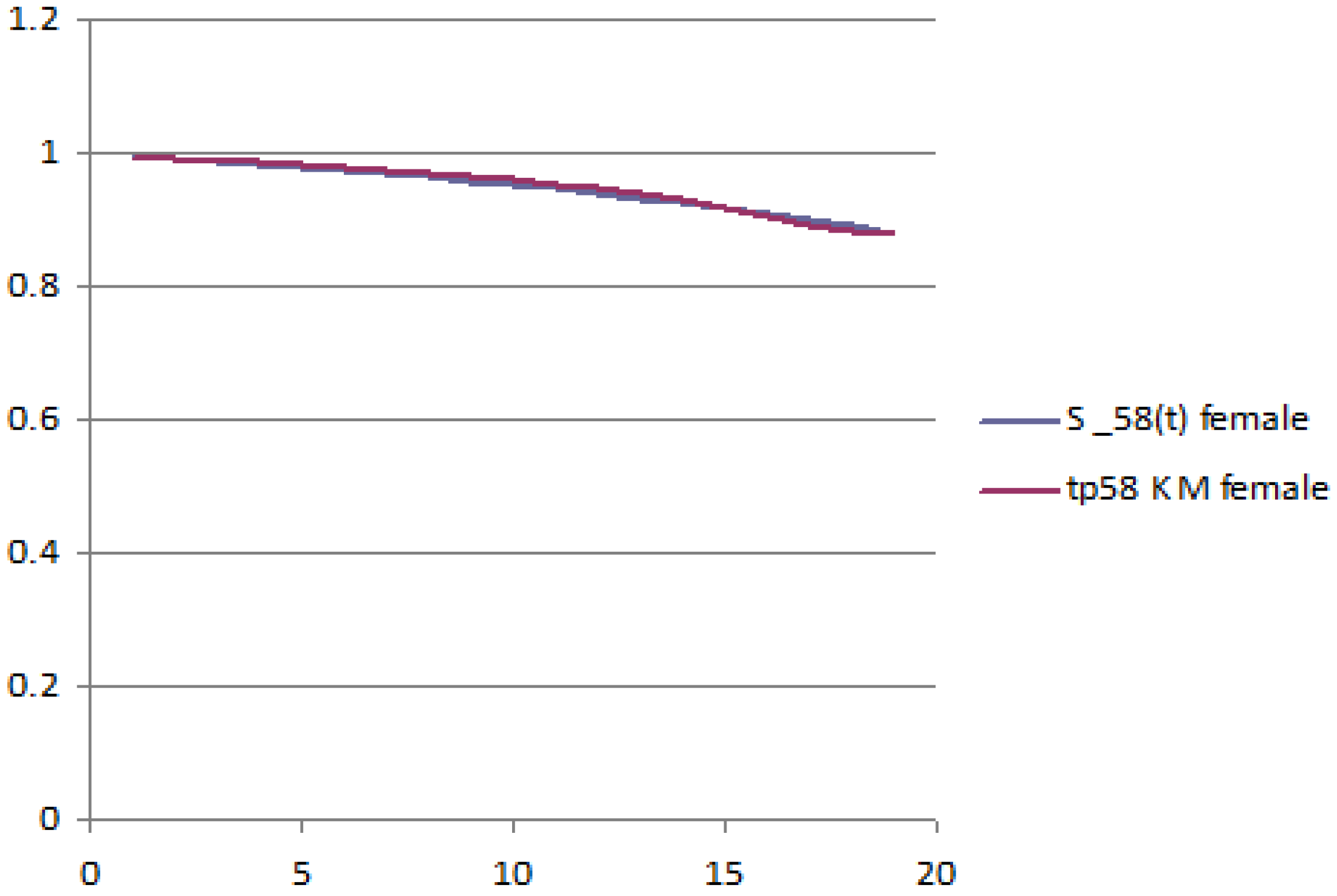
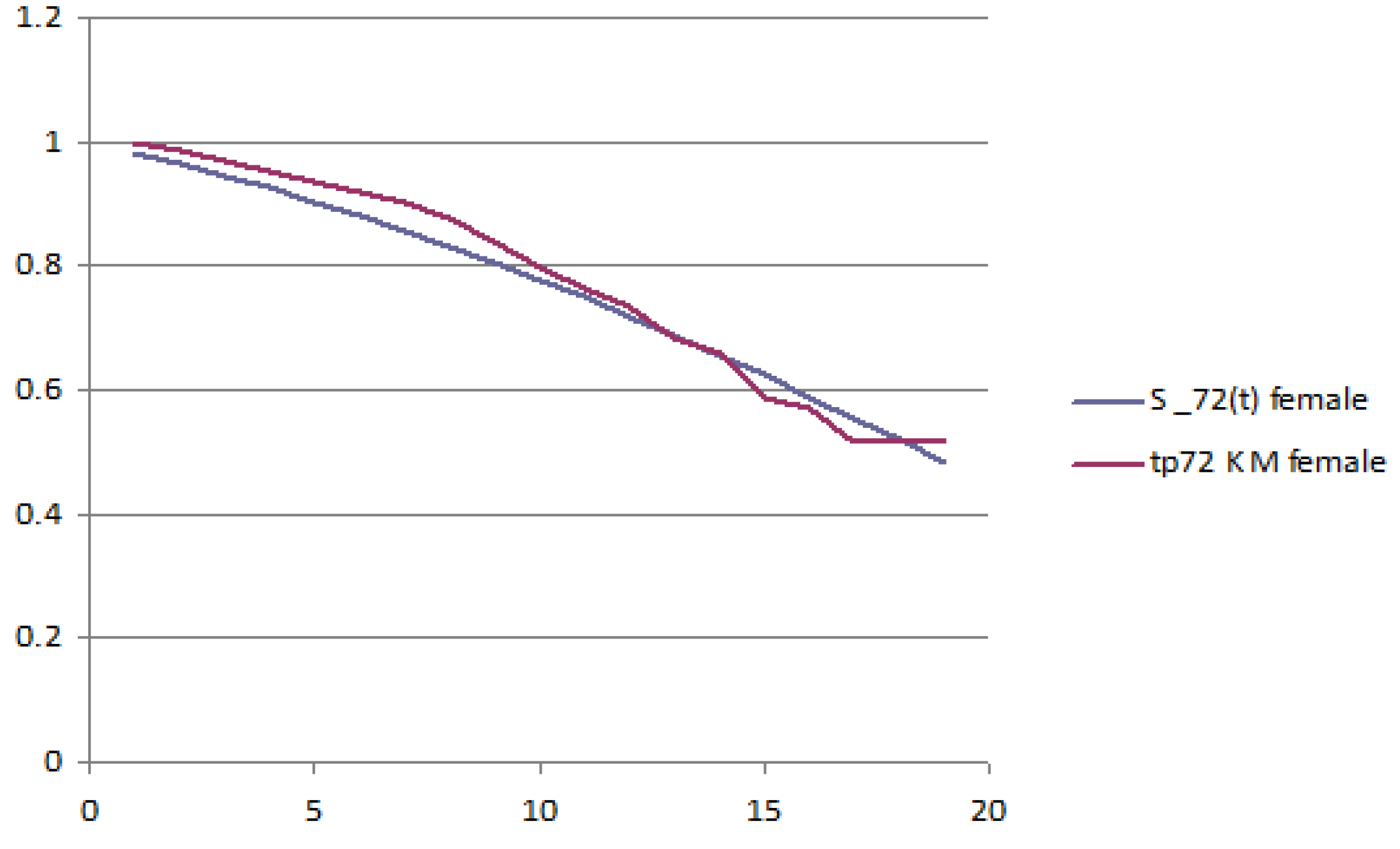
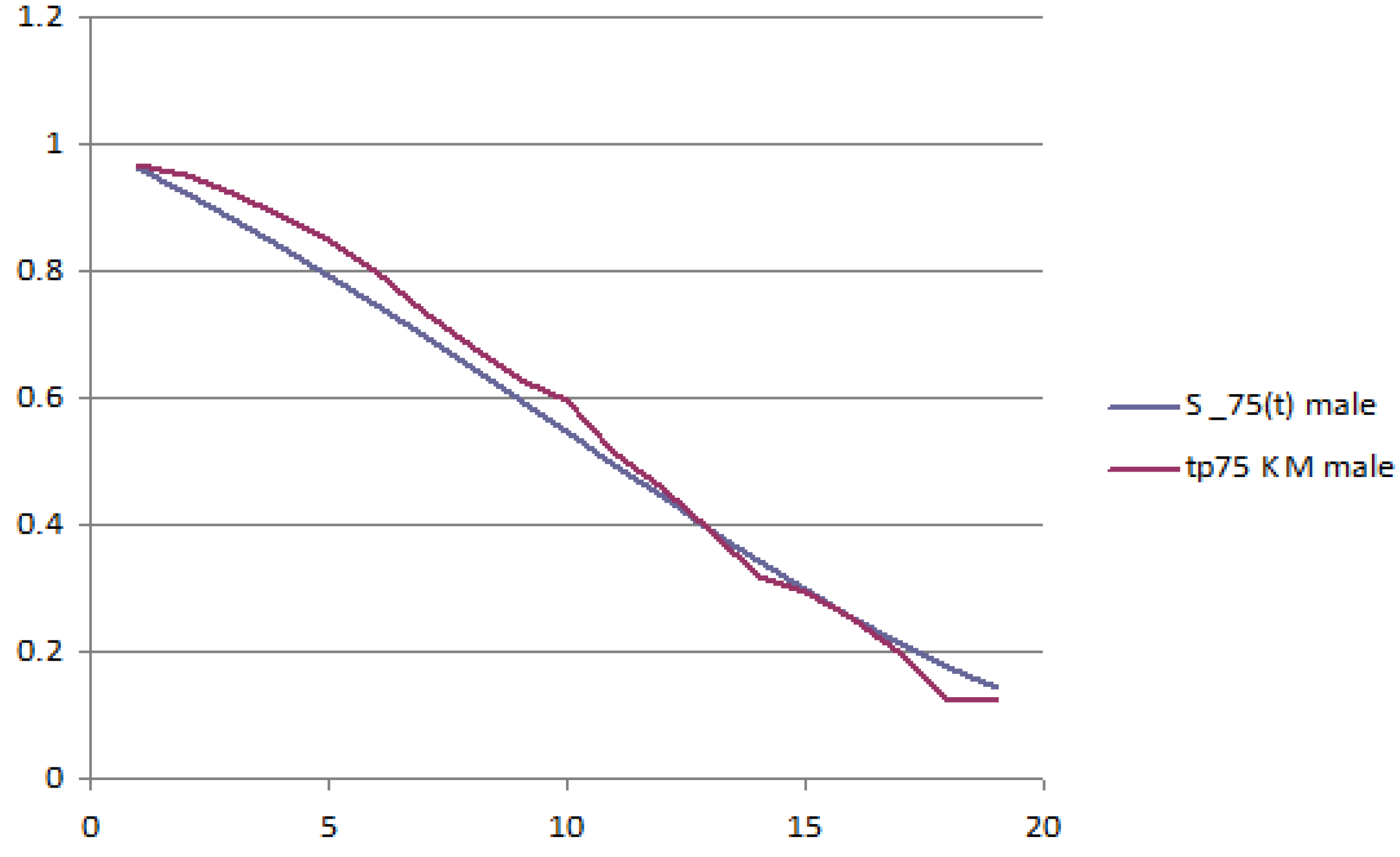
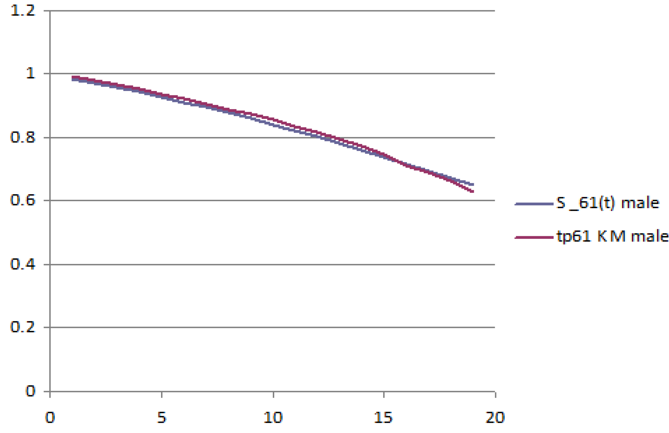
The following figures report the plot of the survival probabilities, grouped by generation and gender. Each figure reports the analytical survival function
for initial age
z and the empirical survival function obtained with the Kaplan–Meier methodology.
Figure 1 and
Figure 2 report the old generation, female and male, respectively;
Figure 3 and
Figure 4 report the young generation, female and male, respectively.
4.2. Decreasing Spouses’ Dependence over Generations
Before calibrating any specific copula, we first compute an empirical estimate
of Kendall’s tau coefficient for each generation. The results are given in
Table 3.
Spouses’ dependence decreases as we consider younger generations. This interesting result is not surprising and is in accordance with the observed increase in the rate of divorces, the creation of extended families, the increased independence of women in the family, and so on. We call this effect the “cohort effect”.
We acknowledge that this result can be subject to skepticism. One might wonder whether the decrease in dependence from older to younger generations is really due to the cohort effect or rather to the age effect, which works as follows. The two generations enter the observation window (from December 1988–December 1993) at different ages. In particular, the old generation enters at ages 75–72 (male-female), while the young generation enters at ages 61–58 (male-female). Thus, the higher spouses’ dependence of the old generation could be partially explained by higher spouses’ dependence of a couple at older ages: one could argue that also for the same generation, spouses’ dependence increases with age or with the duration of marriage or coupling. Because of the age effect, one would expect a higher spouses’ dependence coefficient for the older generation, even without a cohort effect.
Therefore, it seems crucial to disentangle age and cohort effect and to investigate which one is the main explanation of
Table 3. In order to do so, one would need either to observe the same cohort over two different time windows,
i.e., at different ages, or different generations over different windows, but when they have the same initial age. The latter is not feasible with this dataset, because it would require two observation windows distant by 14 years (at least). However, we can observe the same cohort at different ages, as follows:
We create artificially two observation windows out of the unique one, by distinguishing the period 29 December 1988–30 June 1991 from the period 1 July 1991–31 December 1993.
For each cohort, we compute Kendall’s tau in the two sub-windows, in which the same individuals have different initial ages.
Implementing this procedure, we are observing the same generation with different initial ages. The results are reported in
Table 4.
Table 4 shows the unexpected result that for each generation,
τ decreases when time passes, meaning that the spouses’ dependence seems to decrease when the two members of the same cohort become older. This may be due to the small number of couples at disposal in the dataset and to the fact that in order to implement the procedure, we had to further reduce the number of couples in each sub-window. However, had we found the opposite results (
i.e., an increasing
τ), we would have been puzzled by the issue of whether the decreasing Kendall’s tau of
Table 3 was due to cohort effects or to age effects. The likely answer would have been “by both”, and it would have been impossible (with this dataset) to measure the extent of age effect and cohort effect. This would have remained an open issue.
However, the evidence produced by
Table 4 indicates that, for the two generations under scrutiny, increasing age does not imply higher spouses’ dependence. Transferring this conclusion to
Table 3, there seems to be no age effect on the decreasing Kendall’s tau from old generation to young generation. In this dataset, spouses’ dependence decreases when passing from older to younger generations, and this seems to be due only to cohort effects.
We do not intend to claim that, in general, dependence decreases when considering younger generations. This would require extensive investigations that we cannot perform. However, an insurance company endowed with a complete series of data on coupled lives would be able to perform a deeper investigation and separate the age from the generation effect on Kendall’s tau. This would permit one to further support our results that spouses’ dependence is affected by the generations’ effect and decreases when considering younger cohorts.
4.3. Joint Calibration: Archimedean Copulas
Following the method illustrated in
Section 3, for each copula of
Table 1, we calibrate the single-parameter and the two-parameter versions. Given the parameters, we perform a best-fit test among all copulas with the same number of parameters first, among the best-fit copulas with a different number of parameters then.
The results on the log likelihood, AIC and BIC are provided by
Table 5,
Table 6,
Table 7 and
Table 8 (
Table 5 and
Table 6 report data for the old generation;
Table 7 and
Table 8 those for the young generation). In the tables, LH stands for “log likelihood”; 2Ppr stands for “2P product”; 2Pl stands for “2P linear mix”; 2Pg stands for “2P geometrically weighted average”; Fr stands for “Frank copula”; Cl stands for “Clayton copula”; GH stands for “Gumbel–Hougaard copula”; Ne stands for “Nelsen 4.2.20 copula”; and Sp stands for “special copula”. The highest LH, the lowest AIC and the lowest BIC are reported in bold.
The results of the comparison within each class (1P, 2P) can be summarized as follows.
Class 1P: The one-parameter Archimedean family that performs best according to
Table 5 and
Table 7, is the Gumbel–Hougaard for the old generation and the special one for the young generation.
Class 2P: For both generations,
Table 6 and
Table 8 show that the two-parameter family that performs best is the Gumbel–Hougaard linear mix. We observe that the LH of the 2P-product is very similar (and in many cases, identical) to those of the 2P-geometric. For the old generation, the linear-mixing copula is closely followed by the product and geometric Gumbel–Hougaard mixes (as pointed out before, the latter two entail identical copulas): the 2P mixes with the GH copula have a LH much higher than all of the other copulas. This is not the case for the young generation, where the LH are of similar order of magnitude for all copulas and way of mixing.
We see that for the old generation, the best-fit copulas are nested, i.e., the 2P copula is an extension of the 1P, but they are not for the young generation.
The parameters of the best-fit copulas are reported in
Table 9 and
Table 10.
Consistently with the decrease of Kendall’s tau across generations, when the best-fit copula remains the same across generations, the spouses’ dependence parameter is decreasing when passing from the older to the younger generation. Indeed, θ goes from 12.134 to 6.1 for the 2P case.
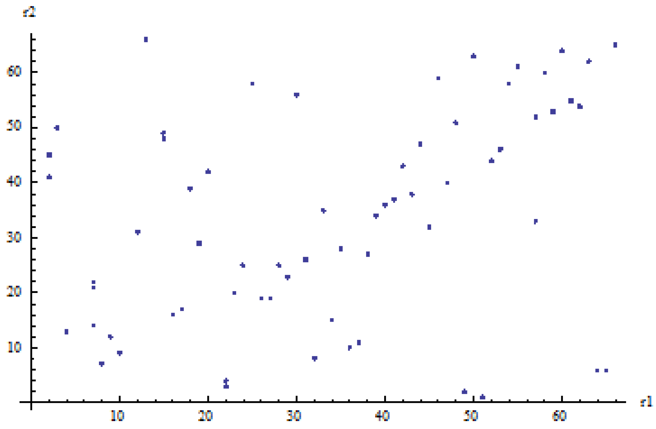
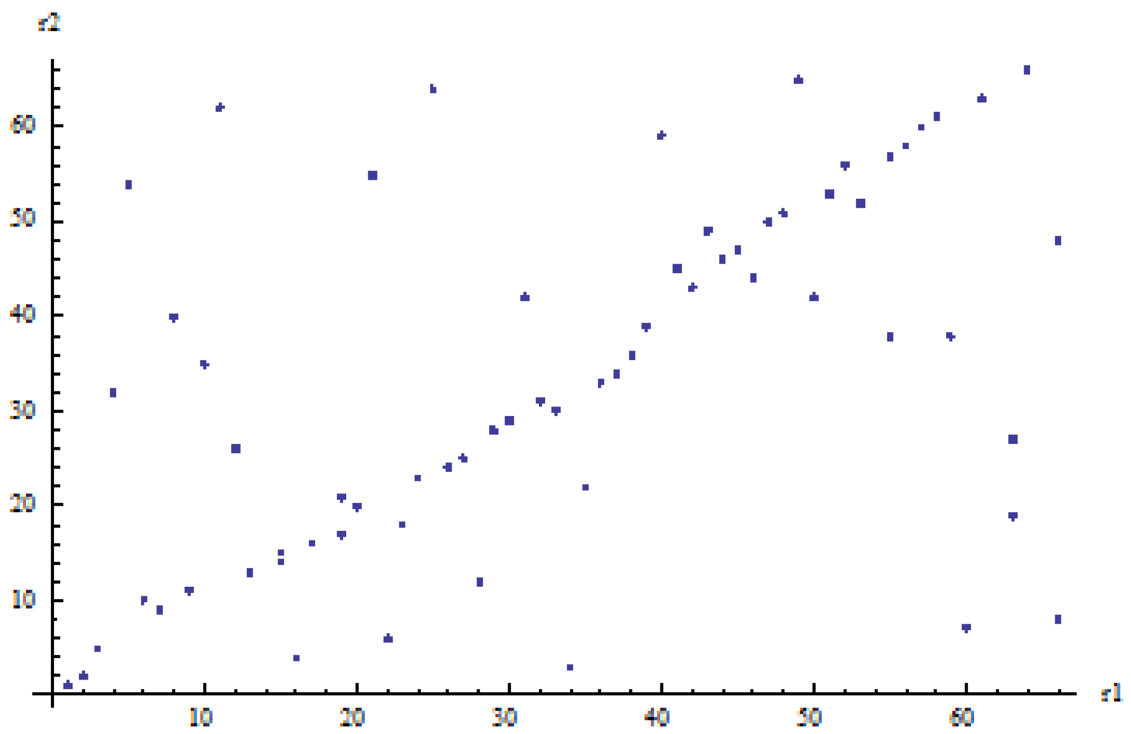
After having established, for a given number of parameters, which copula fits best for each generation, we compare the 1P and 2P versions of each copula in order to assess the correct trade-off between fit and parsimony. We observe that in all cases, the AIC and the BIC values of the 2P copulas are lower than the AIC and BIC values of the corresponding 1P copulas. This indicates that the 2P copulas are more suitable to describe the dependence of this dataset than the 1P copulas. We also note that for the old generation, the passage from 1P to 2P is characterized by a huge gap in the LH. A possible way to explain the superiority of 2P
versus 1P copulas is by observing the scatterplots of the ranked observations for both generations. These are displayed in
Figure 5 (old generation) and
Figure 6 (young generation).
We observe that for both generations, we can distinguish between two subgroups of ranked observations:
points on or close to the main diagonal; considering these points only gives an impression of very strong spouses’ dependence (evidently stronger for the old generation than for the young generation);
the remaining points; considering these points only gives an impression of weak or no spouses’ dependence.
The presence of many observations that display strong spouses’ dependence and others that show no spouses’ dependence can be intuitively captured by mixing a 1P copula with strong spouses’ dependence with the independence copula. Therefore, we are not surprised that the best copula for both generations is the linear-mixing between Gumbel–Hougaard and independence. An intuitive interpretation of the linear mix copula is that a couple has a 100 (55% for the old generation, 37.3% for the young generation) chance of strong dependence, reflected by the points on or near the main diagonal, and a 100 (45% for the old generation, 62.7% for the young generation) chance of no dependence at all. A similar interpretation applies to the geometrically-weighted average (Type 3) after a log transform of the copula, and presumably, although less intuitive, also to the product (Type 1) given that overall, the results in terms of LH and AIC are very similar.
5. Effects of Spouses’ Dependence on Pricing
In this section, we investigate the effect of the spouses’ dependence to the pricing of policies on two lives. We consider a
combined joint life and reversionary annuity , which pays 1 as long as both members are alive and a fraction
R of it (
R stands for “reduction factor”) when only one member of the couple is alive. In this scheme, the last survivor product corresponds to
(the benefit paid remains constant also after the first death), and the joint life annuity corresponds to
(nothing is paid to the last survivor). In practice, such contracts are quite common (see [
3]) for
.
If the interest rate used in the actuarial evaluation is constant at the level
i over the maturity of the contract, the fair price of the reversionary annuity with reduction factor
is:
where
is the discount factor,
is the probability that the benefit
R is paid only to the male,
is the probability that the benefit
R is paid only to the female and
is the probability that the benefit 1 is paid when both are alive. Connecting the survival probabilities needed to the marginal and the joint survival functions, we have:
and also:
Therefore, the price of the combined joint life and reversionary annuity is equal to:
We have implemented the pricing formulas when R takes the values , , , , , , . Results are in the next section.
5.1. Prices of Combined Joint Life and Reversionary Annuities
Table 11 and
Table 12 report the single premia of
R-reversionary annuities for the old generation and the young generation, respectively. The interest rate used is
While the first column reports the value of
R, the second reports the price of the annuity under the independence assumption. For each model specification (1P, 2P), there is a column reporting the best-fit copula price (cum-dependence price) and a column with the ratio between the cum-dependence price and the independence price. In
Table 11 and
Table 12, “GH” stands for “Gumbel-Hougaard”, while in
Table 12 “Spec.” stands for “special”.
Before commenting on dependence effects, notice that for each R and each model specification (1P, 2P), the annuity prices of the young generation are higher than those of the old generation. This is expected, because all survival probabilities are higher for younger insureds. Furthermore, in both tables and for each model specification (1P, 2P), each annuity has a value increasing in R, both under dependence and independency. This is also expected: a higher benefit for the bereaved life implies a higher actuarial value of the benefits to be paid.
Regarding dependence, the reader can notice the following.
For each R and each model specification (1P, 2P), the young generation shows ratios of cum-spouses’ dependence to independence price that are closer to one than those of the old generation. This is a clear consequence of the decreasing τ from old generation to young generation: the milder spouses’ dependence of the young generation generates prices that deviate less from the independence prices than the old generation prices.
In both tables and for each model specification (1P, 2P), the ratio cum-spouses’ dependence/independence is decreasing when
R increases. This can be explained, as well. Let us recall that for
, we have the joint life annuity, and for
, we have the last survivor policy. Then,
R measures the weight given to the last-survivor part of the reversionary annuity, with respect to the joint-life part. When
, positive spouses’ dependence implies that the joint survival probability is higher than in the independence case, leading to a ratio greater than one. At the opposite, when
, we have the last survivor, for which positive spouses’ dependence implies lower survivorship after the spouse’s death, implying ratios lower than one. The values
give all of the intermediate situations between these two extremes. In particular, for
, we still have ratios greater than one; for
, we have ratios lower than one. For
, the ratio is exactly one: the annuity price is unaffected by the level of spouses’ dependence. In fact, due to Equation (
13), the joint survival probability does not enter the premium that reduces to:
The weight given to the last survivor benefit is equal to that given to the joint life annuity, and the two opposite effects of the overestimation and underestimation of the premium perfectly offset each other.
The practical consequence of having ratios greater than one as long as and ratios smaller than one when is that insurance companies, by assuming independence when pricing the former, are under-pricing contracts, while they are over-pricing, or prudentially pricing, the latter. Consider the joint life case. Insurance companies that assume independence are not “on the safe side”. The previous tables give a measure of the lack of safety so obtained. Consistently with Item 1 above, the lack of safety is greater for the older generation. Consider now the last survivor policy, for which insurance companies that assume independence are overpricing the contract. This can be interpreted as a prudential maneuver from the point of view of insurers, and the previous tables give a measure of the extent of prudence so obtained. Consistently with Item 1 above, prudence decreases when the younger generation is selected.
For the old generation, the impact on prices and on the ratio cum-spouses’ dependence/independence is smaller for the 2P copulas than for the 1P copula; the opposite happens for the young generation. As a consequence, for the old generation, the width of the range of prices and ratios when R changes is smaller for the 2P copulas than for the 1P copula; the opposite happens for the young generation. The next item illustrates the mispricing implications of this asymmetry.
Misspecification of the copula produces opposite mispricing effects on the two generations. Indeed, given the assessed superiority of the 2P model with respect to the 1P one, annuity prices show that when the spouses’ dependence is described with a 1P copula rather than with a 2P one, for the old generation, the insurer over-prices annuities with and under-prices annuities with . Opposite results apply to the young generation: when the spouses’ dependence is described with a 1P copula rather than with a 2P one, the insurer under-prices annuities with , and over-prices annuities with . The occurrence of opposite mispricing effects for the two generations could represent a potential for the insurer who wants to natural-hedge reversionary annuities written on one cohort with products on a different cohort.
6. Conclusions
This paper analyzes, first from a statistical, then from a pricing point of view, spouses’ dependence between coupled lives of insureds. We model the marginal distributions of the two spouses with the doubly-stochastic setup and the dependence of the spouses’ lifetimes with the copula approach. We develop the statistical analysis in two directions. We first study the evolution of dependence across generations. We find that on our data, spouses’ dependence decreases when passing from older to younger generations. This decrease in spouses’ dependence is due to the cohort and not to the age effect. We provide a methodology that, if sufficiently rich datasets are available, allows one to separate further age and cohort effects on the evolution of spouses’ dependence. Second, we consider not only a class of single-parameter Archimedean copulas, but also their two-parameter extensions, obtained by mixing with the independence copula. We find that the two-parameter copulas are significantly more suitable to describe spouses’ dependence than single-parameter ones, especially if the extension is the linear-mixing with independence. In this way, our findings echo the results in [
4], even though the datasets are not the same.
When we study the effect of spouses’ dependence on pricing insurance products, we find that dependence matters in pricing annuities on two lives, including joint-life and last-survivor ones. Indeed, when assuming independence, the insurer under-/over-prices such annuities when the benefit payable to the bereaved life is lower/greater than half of the initial benefits payable while both spouses are alive. The misspecification of spouses’ dependence affects in a different way each cohort. Indeed, when the insurer misspecifies the copula (taking one parameter rather than two parameters), the sign in the over- and under-estimation is reversed in the two generations. Since mispricing caused by inaccurate modeling of spouses’ dependence is not uniform across cohorts, the longevity of couples can be hedged away using reinsurance and longevity derivatives on single generations, but also using natural hedging across generations. This is the agenda for future research.
An alternative approach to the study of couples’ dependence could be the multiple state approach. We did not pursue it here because the benchmark literature is copula-based and due to the relative paucity of data, which would make multiple state modeling quite hard. However, we certainly consider it as an alternative worth investigation in the future.


