Macro vs. Micro Methods in Non-Life Claims Reserving (an Econometric Perspective)

Abstract

Traditionally, actuaries have used run-off triangles to estimate reserve (“macro” models, on aggregated data). However, it is possible to model payments related to individual claims. If those models provide similar estimations, we investigate uncertainty related to reserves with “macro” and “micro” models. We study theoretical properties of econometric models (Gaussian, Poisson and quasi-Poisson) on individual data, and clustered data. Finally, applications in claims reserving are considered.

1. Introduction

1.1. Macro and Micro Methods

For more than a century, actuaries have been using run-off triangles to project future payments, in non-life insurance. In the 1930s, [1] formalized this technique that originated from the popular chain ladder algorithm. In the 1990s, [2] proved that the chain ladder estimate can be motivated by a simple stochastic model, and later on [3] provided a comprehensive overview on stochastic models that can be connected with the chain ladder method, including regression models that could be seen as extension of the so-called “factor” methods used in the 1970s.

The terminology of [4] and [5] were used in macro-level models for reserving. In the 1970s, [6] suggested using some marked point process of claims to project future payments, and quantify the reserves. More recently, [7,8,9,10] or [11] (among many others) investigated further some probabilistic micro-level models. These models handle claims related data on an individual basis, rather than aggregating by underwriting year and development period. As mentioned in [12], these methods have not (yet) found great popularity in practice, since they are more difficult to apply. Nevertheless, several papers address that issue, with several stochastic processes to model the dynamics of payments, such as [13]—extended in [14,15] or [16], and more recently [17] and [18].

All macro-level models are based on aggregate data found in a run-off triangle, which is their strength, but also probably their weakness. Indeed, with regulation rules, such as Solvency II or IFRS 4—Phase 2 norms, the goal is no longer to get (only) a best-estimate, but it becomes necessary to have the full conditional distribution of future cash-flows.

Macro-level approaches, such as the popular chain ladder model, have undeniable properties. Those models are part of the actuarial folklore and extensions have been derived to have more general and more realistic models. They are easy to understand, and can be mentioned in financial communication, without disclosing too much information. From a computational perspective, those models can also be implemented in a single spreadsheet and more advanced libraries, such as the ChainLadder package in R can also beused.

Nevertheless, those macro-level models have also major drawbacks, as discussed for instance in [16] or [17], and references therein. More specifically, we wish to highlight two important points:

• Those models neglect a lot of information that is available on a micro-level (per individual claim). Some additional covariates can be used, as well as exposure, etc. In most applications, not only is that information available, but usually, it has a valuable predictive power. To use that additional information, one cannot simply modify macro-level models, and it is necessary to change the general framework of the model. It becomes possible to emphasize large losses and to distinguish them from regular claims, to get more detailed information about future payments, etc.
• As discussed in this paper, macro-level models on aggregated data can be seen as models on clusters and not on individual observations, as we will do with micro-level models. In the context of macro-level models for loss reserving, [3] mention that prediction errors can be large, because of the small number of observations used in run-off triangles and the fact that clusters are usually not homogeneous. Quantifying uncertainty in claim reserving methods is not only important in actuarial practice and to assess accuracy of predictive models, it is also a regulatory issue. Finally, a small sample size can cause a lack of robustness and a risk of over-parametrization for macro-level models.

On the other hand, micro-level models have many pros. They can incorporate micro-level covariates, and model micro-structure of claims development. Thus, they can take into account heterogeneity, structural changes, etc. (see [19] for a discussion). Several studies, with empirical comparisons between macro- and micro-level models (see, e.g., [17]), illustrate that in many scenarios, reserves obtained with micro-level models have higher precision than macro-level ones. Further, since those models are fitted on much more data than aggregated ones, variability of predictions is usually smaller, which increases model robustness and reduces the risk of over-fitting. More specifically, [15] and [16] obtained, on real data analysis, lower variance on the total amount of reserves with “micro” models than with “macro” ones. A natural question is about the generality of such result. Should “micro” model generate less variability than standard “macro” ones? That is the question that initiated this paper.

1.2. Agenda

In Section 2, we detail intuitive results we expect when aggregating data by clusters, moving from micro-level models to macro-level ones. More precisely, we explain why with a linear model and a Poisson regression, macro- and micro-level models are equivalent. We also discuss the case of the Poisson regression model with random intercept. In Section 3, we study “micro” and “macro” models in the context of claims reserving, on real data, as well as simulated ones. More specifically, we present a methodology that allows to generate—by random generation—some micro-datasets obtained from macro-datasets. We investigate also the impact of adding micro-type covariates, allowing for various types of correlations. Finally, we present concluding remarks in Section 4.

2. Clustering in Generalized Linear Mixed Models

In the economic literature, several papers discuss the use of “micro” vs. “macro” data, for instance in the context of unemployment duration in [20] or in the context of inflation in [21]. In [20], it is mentioned that both models are interesting, since “micro” data can be used to capture heterogeneity while “macro” data can capture cycle and more structural patterns. In [21], it is demonstrated that both heterogeneity and aggregation might explain the persistence of inflation at the macroeconomic level.

In order to clarify notation, and make sure that objects are well defined, we use small letters for sample values, e.g., $y_i$, and capital letters for underlying random variables, e.g., $Y_i$ in the sense that $y_i$ is a realisation of random variable $Y_i$. Hence, in the case of the linear model (see Subsection 2.1), we usually assume that $Y_i\sim \mathcal{N}({\mathit{x}}_i^{\mathsf{T}}\mathit{b},{\sigma }^2)$, and then $\widehat{\mathit{b}}$ is the vector of estimated parameters, in the sense that $\widehat{\mathit{b}}={\left(\mathit{x}{\mathit{x}}^{\mathsf{T}}\right)}^{-1}\mathit{x}\mathit{y}$ while $\widehat{\mathit{B}}={\left(\mathit{x}{\mathit{x}}^{\mathsf{T}}\right)}^{-1}\mathit{x}\mathit{Y}$ (here covariates $\mathit{x}$ are given, and non stochastic). Since $\widehat{\mathit{B}}$ is seen as a random variable, we can write $\mathbb{E}\left[\widehat{\mathit{B}}\right]=\mathit{b}$.

With a Poisson regression, $Y_i\sim \mathcal{P}\left({\lambda }_i\right)$ with ${\lambda }_i=exp\left[{\mathit{x}}_i^{\mathsf{T}}\mathit{b}\right]$. In that case, $\text{Var}\left[Y_i\right]=\mathbb{E}\left[Y_i\right]={\lambda }_i$. The estimate parameter $\widehat{\mathit{b}}$ is a function of the observations, $({\mathit{x}}_i,{\mathit{y}}_i)$’s, while $\widehat{\mathit{B}}$ is a function of the observations ${\mathit{x}}_i$ and of the random variable ${\mathit{Y}}_i$. In the context of the Poisson regression, recall that $\mathbb{E}\left[\widehat{\mathit{B}}\right]\to \mathit{b}$ as n, the number of observations, goes to infinity. With a quasi-Poisson regression, $Y_i$ does not have, per se, a proper distribution. Nevertheless, its moments are well defined, in the sense that $\text{Var}\left[Y_i\right]=\phi \mathbb{E}\left[Y_i\right]=\phi {\lambda }_i$, where φ denotes the dispersion parameter (see Subsection 2.2). For convenience, we will denote $Y_i\sim q\mathcal{P}\left({\lambda }_i\right)$, with an abuse of notation.

In this section, we will derive some theoretical results regarding aggregation in econometric models.

2.1. The Multiple Linear Regression Model

For a $(k+1)\times 1$ vector of parameters $\mathit{a}$, we consider a (multiple) linear regression model,

$$\begin{array}{cc}\hfill y_{i,g}& ={\mathit{x}}_g^{\mathsf{T}}\mathit{a}+{\epsilon }_{i,g}\hfill \\ \hfill \mathit{a}& ={\left[\begin{array}{ccc}{a}_1& \dots & a_{k+1}\end{array}\right]}^{\mathsf{T}}{\mathit{x}}_g={\left[\begin{array}{ccc}{x}_{g,1}& \dots & x_{g,k+1}\end{array}\right]}^{\mathsf{T}}\hfill \end{array}$$

(1)

where observations belong to a cluster g and are indexed by i within a cluster g, $i=1,\dots ,n_g$, $g=1,\dots ,m$. Assume further assumptions of the classical linear regression model [22], i.e.,

(LRM1)

no multicollinearity in the data matrix;

(LRM2)

exogeneity of the independent variables $\mathbb{E}\left[{\epsilon }_{i,g}|{\mathit{x}}_g\right]=0$, $i=1,\dots ,n_g$, $g=1,\dots ,m$; and

(LRM3)

homoscedasticity and nonautocorrelation of error terms with $\text{Var}\left[{\epsilon }_{i,g}\right]={\sigma }^2$.

Stacking observations within a cluster yield the following model

$$\begin{array}{cc}\hfill {\overline{y}}_g& ={\mathit{x}}_g^{\mathsf{T}}\mathit{b}+e_g\hfill \end{array}$$

(2)

where

$${\overline{y}}_g=\frac{1}{n_g}\sum _i{n}_{i,g} \mathrm{and} \mathit{b}={\left[\begin{array}{ccc}{b}_1& \dots & b_{k+1}\end{array}\right]}^{\mathsf{T}}$$

with similar assumptions except for $\text{Var}\left[e_g\right]={\sigma }^2/n_g$. Those two models are equivalent, in the sense that the following proposition holds.

Proposition 1. 

Model (1) on a micro level and Model (2) on a macro level are equivalent, in the sense that

(i) 

${\widehat{\mathit{a}}}_{OLS}={\widehat{\mathit{b}}}_{OLS}$ when weights $n_g$ are used in Model (2); and

(ii) 

${\displaystyle \sum _{i,g}{\widehat{y}}_{i,g}=\sum _g{\widehat{y}}_g}$ where $y_g=n_g{\overline{y}}_g$.

Proof. 

(i)

The ordinary least-squares estimator for $\mathit{a}$ - from Model (1)—is defined as

$$\widehat{\mathit{a}}=\underset{\mathit{a}}{\text{argmin}}\left\{\sum _{i,g}{\left(y_{i,g}-{\mathit{x}}_g^{\mathsf{T}}\mathit{a}\right)}^2\right\}$$

(3)

which can also be written

$$\widehat{\mathit{a}}=\underset{\mathit{a}}{\text{argmin}}\left\{\sum _{i,g}{\left(y_{i,g}-{\overline{y}}_g+{\overline{y}}_g-{\mathit{x}}_g^{\mathsf{T}}\mathit{a}\right)}^2\right\}.$$

(4)

Now, observe that

$$\begin{array}{cc}\hfill \sum _{i,g}{\left(y_{i,g}-{\overline{y}}_g+{\overline{y}}_g-{\mathit{x}}_g^{\mathsf{T}}\mathit{a}\right)}^2& =\sum _{i,g}{(y_{i,g}-{\overline{y}}_g)}^2+{({\overline{y}}_g-{\mathit{x}}_g^{\mathsf{T}}\mathit{a})}^2\hfill \\ & \phantom{=}+2(y_{i,g}-{\overline{y}}_g)({\overline{y}}_g-{\mathit{x}}_g^{\mathsf{T}}\mathit{a})\hfill \end{array}$$

where the first term is independent of $\mathit{a}$ (and can be removed from the optimization program), and the term with cross-elements sums to 0. Hence,

$$\widehat{\mathit{a}}=\underset{\mathit{a}}{\text{argmin}}\left\{\sum _{i,g}{({\overline{y}}_g-{\mathit{x}}_g^{\mathsf{T}}\mathit{a})}^2\right\}=\underset{\mathit{a}}{\text{argmin}}\left\{\sum _g{n}_g{({\overline{y}}_g-{\mathit{x}}_g^{\mathsf{T}}\mathit{a})}^2\right\}=\widehat{\mathit{b}}$$

(5)

where $\widehat{\mathit{b}}$ is the least square estimator of $\mathit{b}$ from Model (2), when weights $n_g$ are considered.

(ii)

If we consider the sum of predicted values, observe that

$$\sum _{i,g}{\widehat{y}}_{i,g}=\sum _g{n}_g{\mathit{x}}_g^{\mathsf{T}}\widehat{\mathit{a}}=\sum _g{n}_g\underset{{\widehat{\overline{y}}}_g}{\underbrace{{\mathit{x}}_g^{\mathsf{T}}\widehat{\mathit{b}}}}=\sum _g{\widehat{y}}_g$$

(6)

Hence, the sum of predictions obtained from Model (1) is the same as the sum of predictions obtained from Model (2), even if partial sums are considered.

  ☐

In the proposition above, the equality should be understood as the equality between estimators. Hence we have the following corollary.

Corollary 2. 

We define the following matrices

$$\begin{array}{cc}\hfill {\mathit{Y}}_g& ={\left[\begin{array}{ccc}{Y}_{1,g}& \dots & Y_{n_g,g}\end{array}\right]}^{\mathsf{T}}\mathit{Y}={\left[\begin{array}{ccc}{\mathit{Y}}_1^{\mathsf{T}}& \dots & {\mathit{Y}}_m^{\mathsf{T}}\end{array}\right]}^{\mathsf{T}}\overline{\mathit{Y}}={\left[\begin{array}{ccc}{\overline{Y}}_1& \dots & {\overline{Y}}_m\end{array}\right]}^{\mathsf{T}}\hfill \\ \hfill {\mathit{\epsilon }}_g& ={\left[\begin{array}{ccc}{\epsilon }_{1,g}& \dots & {\epsilon }_{n_g,g}\end{array}\right]}^{\mathsf{T}}\mathit{\epsilon }={\left[\begin{array}{ccc}{\epsilon }_1& \dots & {\epsilon }_m\end{array}\right]}^{\mathsf{T}}\mathit{e}={\left[\begin{array}{ccc}{e}_1& \dots & e_m\end{array}\right]}^{\mathsf{T}}\hfill \\ \hfill {\mathit{x}}_g^{n_g}& =\underset{n_g\mathit{times}}{\underbrace{\left[\begin{array}{ccc}{\mathit{x}}_g& \dots & {\mathit{x}}_g\end{array}\right]}}\mathit{x}=\left[\begin{array}{ccc}{\mathit{x}}_1^{n_1}& \dots & {\mathit{x}}_m^{n_m}\end{array}\right]\overline{\mathit{x}}=\left[\begin{array}{ccc}{\mathit{x}}_1^1& \dots & {\mathit{x}}_m^1\end{array}\right]\hfill \end{array}$$

the $(1\times n_g)$ vectors ${\mathbf{1}}_{n_g}=\left[\begin{array}{ccc}1& \dots & 1\end{array}\right]$ and ${\mathbf{0}}_{n_g}=\left[\begin{array}{ccc}0& \dots & 0\end{array}\right]$, and the matrix

$$\begin{array}{cc}\hfill \mathbf{1}& =\left[\begin{array}{cccc}{\mathbf{1}}_{n_1}& {\mathbf{0}}_{n_2}& \dots & {\mathbf{0}}_{n_m}\\ {\mathbf{0}}_{n_1}& {\mathbf{1}}_{n_2}& \dots & {\mathbf{0}}_{n_m}\\ ⋮& ⋮& \ddots & ⋮\\ {\mathbf{0}}_{n_1}& {\mathbf{0}}_{n_2}& \dots & {\mathbf{1}}_{n_m}\end{array}\right]\hfill \end{array}$$

The OLS estimators are given by

$$\begin{array}{cc}\hfill {\widehat{\mathit{A}}}_{OLS}& =\underset{\mathit{a}}{\text{argmin}}\left\{{\left(\mathit{Y}-{\mathit{x}}^{\mathsf{T}}\mathit{a}\right)}^{\mathsf{T}}\left(\mathit{Y}-{\mathit{x}}^{\mathsf{T}}\mathit{a}\right)\right\}\hfill \\ & ={\left(\mathit{x}{\mathit{x}}^{\mathsf{T}}\right)}^{-1}\mathit{x}\mathit{Y}\hfill \end{array}$$

$$\begin{array}{cc}\hfill {\widehat{\mathit{B}}}_{OLS}& =\underset{\mathit{b}}{\text{argmin}}\left\{{\left(\left(\sqrt{\mathbf{1}{\mathbf{1}}^{\mathsf{T}}}\right)\overline{\mathit{Y}}-\sqrt{\mathbf{1}{\mathbf{1}}^{\mathsf{T}}}{\overline{\mathit{x}}}^{\mathsf{T}}\mathit{b}\right)}^{\mathsf{T}}\left(\left(\sqrt{\mathbf{1}{\mathbf{1}}^{\mathsf{T}}}\right)\overline{\mathit{Y}}-\left(\sqrt{\mathbf{1}{\mathbf{1}}^{\mathsf{T}}}\right){\overline{\mathit{x}}}^{\mathsf{T}}\mathit{b}\right)\right\}\hfill \\ & ={\left(\overline{\mathit{x}}\mathbf{1}{\mathbf{1}}^{\mathsf{T}}{\overline{\mathit{x}}}^{\mathsf{T}}\right)}^{-1}\overline{\mathit{x}}\mathbf{1}{\mathbf{1}}^{\mathsf{T}}\overline{\mathit{Y}}\hfill \end{array}$$

Model (1) on a micro level and Model (2) on a macro level are equivalent, in the sense that

(i) 

$\mathbb{E}\left[{\widehat{\mathit{A}}}_{OLS}\right]=\mathbb{E}\left[{\widehat{\mathit{B}}}_{OLS}\right]$ and $Var\left[{\widehat{\mathit{A}}}_{OLS}\right]=Var\left[{\widehat{\mathit{B}}}_{OLS}\right]$, when weights $n_g$ are used in Model (2); and

(ii) 

${\displaystyle \mathbb{E}\left[\sum _{i,g}{\widehat{Y}}_{i,g}\right]=\mathbb{E}\left[\sum _g{\widehat{Y}}_g\right]}$ and ${\displaystyle Var\left[\sum _{i,g}{\widehat{Y}}_{i,g}\right]=Var\left[\sum _g{\widehat{Y}}_g\right]}$.

Proof. 

Straightforward calculations lead to ${\left(\mathbf{1}{\mathbf{1}}^{\mathsf{T}}\right)}^{-1}\mathbf{1}\mathit{Y}=\overline{\mathit{Y}}$ and $\overline{\mathit{x}}\mathbf{1}=\mathit{x}$.

(i)

Let

$$\begin{array}{cc}\hfill \mathbb{E}\left[{\widehat{\mathit{B}}}_{OLS}\right]& ={\left(\overline{\mathit{x}}\mathbf{1}{\mathbf{1}}^{\mathsf{T}}{\overline{\mathit{x}}}^{\mathsf{T}}\right)}^{-1}\overline{\mathit{x}}\mathbf{1}{\mathbf{1}}^{\mathsf{T}}\mathbb{E}\left[\overline{\mathit{Y}}\right]\hfill \\ & ={\left(\overline{\mathit{x}}\mathbf{1}{\mathbf{1}}^{\mathsf{T}}{\overline{\mathit{x}}}^{\mathsf{T}}\right)}^{-1}\overline{\mathit{x}}\mathbf{1}{\mathbf{1}}^{\mathsf{T}}{\left(\mathbf{1}{\mathbf{1}}^{\mathsf{T}}\right)}^{-1}\mathbf{1}\mathbb{E}\left[\mathit{Y}\right]\hfill \\ & ={\left(\mathit{x}{\mathit{x}}^{\mathsf{T}}\right)}^{-1}\mathit{x}\mathbb{E}\left[\mathit{Y}\right]=\mathbb{E}\left[{\widehat{\mathit{A}}}_{OLS}\right]\hfill \end{array}$$

For the equality of variances, we have

$$\begin{array}{cc}& \text{Var}\left[{\widehat{\mathit{B}}}_{OLS}\right]\hfill \\ & ={\left(\overline{\mathit{x}}\mathbf{1}{\mathbf{1}}^{\mathsf{T}}{\overline{\mathit{x}}}^{\mathsf{T}}\right)}^{-1}\overline{\mathit{x}}\mathbf{1}{\mathbf{1}}^{\mathsf{T}}\text{Var}\left[\overline{\mathit{Y}}\right]{\left({\left(\overline{\mathit{x}}\mathbf{1}{\mathbf{1}}^{\mathsf{T}}{\overline{\mathit{x}}}^{\mathsf{T}}\right)}^{-1}\overline{\mathit{x}}\mathbf{1}{\mathbf{1}}^{\mathsf{T}}\right)}^{\mathsf{T}}\hfill \\ & ={\left(\overline{\mathit{x}}\mathbf{1}{\mathbf{1}}^{\mathsf{T}}{\overline{\mathit{x}}}^{\mathsf{T}}\right)}^{-1}\overline{\mathit{x}}\mathbf{1}{\mathbf{1}}^{\mathsf{T}}{\left(\mathbf{1}{\mathbf{1}}^{\mathsf{T}}\right)}^{-1}\mathbf{1}\text{Var}\left[\mathit{Y}\right]{\mathbf{1}}^{\mathsf{T}}{\left({\left(\mathbf{1}{\mathbf{1}}^{\mathsf{T}}\right)}^{-1}\right)}^{\mathsf{T}}{\left({\left(\overline{\mathit{x}}\mathbf{1}{\mathbf{1}}^{\mathsf{T}}{\overline{\mathit{x}}}^{\mathsf{T}}\right)}^{-1}\overline{\mathit{x}}\mathbf{1}{\mathbf{1}}^{\mathsf{T}}\right)}^{\mathsf{T}}\hfill \\ & ={\left(\mathit{x}{\mathit{x}}^{\mathsf{T}}\right)}^{-1}\mathit{x}\text{Var}\left[\mathit{Y}\right]{\mathit{x}}^{\mathsf{T}}{\left({\left(\mathit{x}{\mathit{x}}^{\mathsf{T}}\right)}^{-1}\right)}^{\mathsf{T}}\hfill \\ & =\text{Var}\left[{\widehat{\mathit{A}}}_{OLS}\right]\hfill \end{array}$$

(ii)

Let

$$\begin{array}{cc}\hfill \mathbb{E}\left[\sum _g{\widehat{Y}}_g\right]& =\mathbb{E}\left[{\mathbf{1}}_m\mathbf{1}{\mathbf{1}}^{\mathsf{T}}\widehat{\overline{\mathit{Y}}}\right]=\mathbb{E}\left[{\mathbf{1}}_m\mathbf{1}{\mathbf{1}}^{\mathsf{T}}{\overline{\mathit{x}}}^{\mathsf{T}}\widehat{\mathit{B}}\right]\hfill \\ & =\mathbb{E}\left[{\mathbf{1}}_m\mathbf{1}{\mathbf{1}}^{\mathsf{T}}{\overline{\mathit{x}}}^{\mathsf{T}}\widehat{\mathit{A}}\right]=\mathbb{E}\left[{\mathbf{1}}_n{\mathit{x}}^{\mathsf{T}}\widehat{\mathit{A}}\right]\hfill \\ & =\mathbb{E}\left[{\mathbf{1}}_n\widehat{\mathit{Y}}\right]=\mathbb{E}\left[\sum _{i,g}{Y}_{i,g}\right]\hfill \end{array}$$

The proof of the equality of variances is similar.

 ☐

2.2. The Quasi-Poisson Regression

A similar result can be obtained in the context of Poisson regressions. A generalized linear model [23] is made up of a linear predictor ${\mathit{x}}^{\mathsf{T}}\mathit{b}$, a link function that describes how the expected value depends on this linear predictor and a variance function that describes how the variance depends on the expected value $\text{Var}\left[Y\right]=\phi V\left(\mathbb{E}\left[Y\right]\right)$, where $\phi$ denotes the dispersion parameter. For the Poisson model, the variance is equal to the mean, i.e., $\phi =1$ and $V\left(\mathbb{E}\left[Y\right]\right)=\mathbb{E}\left[Y\right]$. This may be too restrictive for many actuarial illustrations, which often show more variation than given by expected values. We use the term over-dispersed for a model where the variance exceeds the expected value. A common way to deal with over-dispersion is a quasi-likelihood approach (see [23] for further discussion) where a model is characterized by its first two moments.

Consider either a Poisson regression model, or a quasi-Poisson one,

$$Y_{i,g}\sim \mathcal{P}\left({\lambda }_{i,g}\right)\text{or}{Y}_{i,g}\sim q\mathcal{P}\left({\lambda }_{i,g}\right)$$

(7)

In the case of a Poisson regression,

$$\mathbb{E}\left[Y_{i,g}\right]={\lambda }_{i,g}=exp[{\mathit{x}}_g^{\mathsf{T}}\mathit{a}+ln(1/n_g)]\text{and}\text{Var}\left[Y_{i,g}\right]={\lambda }_{i,g}$$

(8)

and in the context of a quasi-Poisson regression,

$$\mathbb{E}\left[Y_{i,g}\right]={\lambda }_{i,g}=exp[{\mathit{x}}_g^{\mathsf{T}}\mathit{a}+ln(1/n_g)]\text{and}\text{Var}\left[Y_{i,g}\right]={\phi }_{\text{micro}}{\lambda }_{i,g}$$

(9)

with ${\phi }_{\text{micro}}>0$ for a quasi-Poisson regression (${\phi }_{\text{micro}}>1$ for over-dispersion). Here again, stacking observations within a cluster yield the following model (on the sum and not the average value, to have a valid interpretation with a Poisson distribution)

$$Y_g=\sum _i{Y}_{i,g}\sim \mathcal{P}\left({\lambda }_g\right)\text{or}{Y}_g\sim q\mathcal{P}\left({\lambda }_g\right)$$

(10)

In the context of a Poisson regression,

$$\mathbb{E}\left[Y_g\right]={\lambda }_g=exp\left[{\mathit{x}}_g^{\mathsf{T}}\mathit{b}\right]\text{and}\text{Var}\left[Y_g\right]={\lambda }_g$$

and in the context of a quasi-Poisson regression,

$$\mathbb{E}\left[Y_g\right]={\lambda }_g=exp\left[{\mathit{x}}_g^{\mathsf{T}}\mathit{b}\right]\text{and}\text{Var}\left[Y_g\right]={\phi }_{\text{macro}}{\lambda }_g$$

(11)

with ${\phi }_{\text{macro}}>0$ for a quasi-Poisson regression. Here again, those two models (“micro” and “macro”) are equivalent, in the sense that the following proposition holds.

Proposition 3. 

Model (7) on a micro level and Model (10) on a macro level are equivalent in the sense that

(i) 

${\widehat{\mathit{a}}}_{MLE}={\widehat{\mathit{b}}}_{MLE}$; and

(ii) 

${\displaystyle \sum _{i,g}{\widehat{y}}_{i,g}=\sum _g{\widehat{y}}_g}$.

Proof. 

(i)

Maximum likelihood estimator of $\mathit{a}$ is the solution of

$$\begin{array}{cc}\hfill \sum _{i,g}\left(\frac{y_{i,g}-exp\left[{\mathit{x}}_g^{\mathsf{T}}\mathit{a}\right]}{{\phi }_{\text{micro}}}\right){\mathit{x}}_g& =\mathbf{0}\hfill \end{array}$$

or equivalently

$$\begin{array}{cc}\hfill \sum _{i,g}\left(y_{i,g}-exp\left[{\mathit{x}}_g^{\mathsf{T}}\mathit{a}\right]\right){\mathit{x}}_g& =\mathbf{0}\hfill \end{array}$$

With offsets ${\lambda }_g^{*}=exp[{\mathit{x}}_g^{\mathsf{T}}\mathit{b}+log\left(n_g\right)]$, $g=1,\dots ,m$, maximum likelihood estimator of $\mathit{b}$ is the solution (as previously, we can remove ${\phi }_{\text{macro}}$) of

$$\begin{array}{cc}\hfill \sum _g\left(y_g-n_{g}exp\left[{\mathit{x}}_g^{\mathsf{T}}\mathit{b}\right]\right){\mathit{x}}_g& =0\hfill \end{array}$$

$$\begin{array}{cc}\hfill \sum _{i,g}\left(y_{i,g}-exp\left[{\mathit{x}}_g^{\mathsf{T}}\mathit{b}\right]\right){\mathit{x}}_g& =0\hfill \end{array}$$

Hence, $\widehat{\mathit{a}}=\widehat{\mathit{b}}$, as (unique) solutions of the same system of equations.

(ii)

The sum of predicted values is

$$\begin{array}{cc}\hfill \sum _{i,g}{\widehat{y}}_{i,g}& =\sum _g{n}_g{\widehat{\lambda }}_{i,g}=\sum _g{n}_{g}exp\left[{\mathit{x}}_g^{\mathsf{T}}\widehat{\mathit{a}}\right]=\sum _g{n}_{g}exp\left[{\mathit{x}}_g^{\mathsf{T}}\widehat{\mathit{b}}\right]\hfill \\ & =\sum _{g}exp[{\mathit{x}}_g^{\mathsf{T}}\widehat{\mathit{b}}+log\left(n_g\right)]=\sum _g{\widehat{\lambda }}_g^{*}=\sum _g{\widehat{y}}_g\hfill \end{array}$$

☐

Nevertheless, as we will see later on, the Corollary obtained in the context of a Gaussian linear model does not hold in the context of a quasi-Poisson regression.

Corollary 4. 

Model (7) on a micro level and Model (10) on a macro level are asymptotically equivalent for Poisson regressions, in the sense that

(i) 

$\mathbb{E}\left[{\widehat{\mathit{A}}}_{MLE}\right]=\mathbb{E}\left[{\widehat{\mathit{B}}}_{MLE}\right]$ and $Var\left[{\widehat{\mathit{A}}}_{MLE}\right]=Var\left[{\widehat{\mathit{B}}}_{MLE}\right]$, when n goes to infinity; and

(ii) 

${\displaystyle \mathbb{E}\left[\sum _{i,g}{\widehat{Y}}_{i,g}\right]=\mathbb{E}\left[\sum _g{\widehat{Y}}_g\right]}$ and ${\displaystyle Var\left[\sum _{i,g}{\widehat{Y}}_{i,g}\right]=Var\left[\sum _g{\widehat{Y}}_g\right]}$, when n goes to infinity.

Proof. 

(i)

A classical result of asymptotic theory for maximum likelihood estimators indicates that, under mild regularity conditions, $\mathbb{E}\left[{\widehat{\mathit{A}}}_{MLE}\right]\to \mathit{a}$ and $\mathbb{E}\left[{\widehat{\mathit{B}}}_{MLE}\right]\to \mathit{b}$ as $n\to \infty$. Since $\mathit{a}=\mathit{b}$, we have $\mathbb{E}\left[{\widehat{\mathit{B}}}_{MLE}\right]=\mathbb{E}\left[{\widehat{\mathit{A}}}_{MLE}\right]$ when $n\to \infty$. For Model (7), the Fisher information matrix is $\mathit{I}\left(\mathit{A}\right)=\mathit{x}\mathit{W}{\mathit{x}}^{\mathsf{T}}$ and, when $n\to \infty$, $\text{Var}\left[\widehat{\mathit{A}}\right]\to {\left(\mathit{x}\mathit{W}{\mathit{x}}^{\mathsf{T}}\right)}^{-1}$, where $\mathit{W}=\text{diag}(({\lambda }_1/n_1){\mathbf{1}}_{n_1},\dots ,({\lambda }_m/n_m){\mathbf{1}}_{n_m})$. For Model (10), we have $\mathit{I}\left(\mathit{B}\right)=\overline{\mathit{x}}\mathbf{1}\mathit{W}{\mathbf{1}}^{\mathsf{T}}{\overline{\mathit{x}}}^{\mathsf{T}}=\mathit{x}\mathit{W}{\mathit{x}}^{\mathsf{T}}$ and, when $n\to \infty$, $\text{Var}\left[\widehat{\mathit{B}}\right]\to {\left(\mathit{x}\mathit{W}{\mathit{x}}^{\mathsf{T}}\right)}^{-1}$.

(ii)

By using a similar argument, we have when n goes to infinity

$$\begin{array}{cc}\hfill \mathbb{E}\left[\sum _g{\widehat{Y}}_g\right]& =\mathbb{E}\left[{\mathbf{1}}_m\mathbf{1}{\mathbf{1}}^{\mathsf{T}}\widehat{\overline{\mathit{Y}}}\right]={\mathbf{1}}_m\mathbf{1}{\mathbf{1}}^{\mathsf{T}}{M}_{\widehat{\mathit{B}}}\left({\overline{\mathit{x}}}^{\mathsf{T}}\right)\hfill \\ & ={\mathbf{1}}_m\mathbf{1}{\mathbf{1}}^{\mathsf{T}}{M}_{\widehat{\mathit{A}}}\left({\overline{\mathit{x}}}^{\mathsf{T}}\right)=\mathbb{E}\left[{\mathbf{1}}_n{\mathbf{1}}^{\mathsf{T}}{e}^{{\overline{\mathit{x}}}^{\mathsf{T}}\widehat{\mathit{A}}}\right]=\mathbb{E}\left[{\mathbf{1}}_n{e}^{{\mathit{x}}^{\mathsf{T}}\widehat{\mathit{A}}}\right]\hfill \\ & =\mathbb{E}\left[{\mathbf{1}}_n\widehat{\mathit{Y}}\right]=\mathbb{E}\left[\sum _{i,g}{\widehat{Y}}_{g,i}\right]\hfill \end{array}$$

☐

In small or moderate-sized samples, it should be noted that $\widehat{\mathit{A}}$ and $\widehat{\mathit{B}}$ may be biased for $\mathit{A}$ and $\mathit{B}$, respectively. Generally, this bias is negligible compared with the standard errors (see [24,25]).

In the quasi-Poisson micro-level model (from Model (7)), as discussed above, the estimator of $\mathit{a}$ is the solution of the quasi-score function

$$\begin{array}{cc}\hfill \sum _{i,g}\left(\frac{y_{i,g}-{\lambda }_{i,g}}{{\phi }_{micro}}\right){\mathit{x}}_g& =0\hfill \end{array}$$

which implies ${\widehat{\mathit{a}}}_{QLE}={\widehat{\mathit{a}}}_{MLE}$. The classical Pearson estimator for the dispersion parameter ${\phi }_{\text{micro}}$ is

$$\begin{array}{cc}\hfill {\widehat{\phi }}_{micro}& =\sum _{i,g}\frac{{\left(y_{i,g}-{\widehat{y}}_{i,g}\right)}^2/{\widehat{y}}_{i,g}}{{\sum }_g{n}_g-(k+1)}=\sum _{i,g}\frac{{\left(n_g{y}_{i,g}-{\widehat{y}}_g\right)}^2/n_g{\widehat{y}}_g}{{\sum }_g{n}_g-(k+1)}\hfill \end{array}$$

Empirical evidence (see [26]) support the use of the Pearson estimator for estimating $\phi$ because it is the most robust against the distributional assumption. In a similar way, the quasi-Poisson macro-level model (from Model (10)), the estimator of $\mathit{b}$ is the solution of

$$\begin{array}{cc}\hfill \sum _g\left(\frac{y_g-{\lambda }_g}{{\phi }_{macro}}\right){\mathit{x}}_g& =0\hfill \end{array}$$

which implies here also ${\widehat{\mathit{b}}}_{QLE}={\widehat{\mathit{b}}}_{MLE}$. The dispersion parameter $\phi$ is estimated by

$$\begin{array}{cc}\hfill {\widehat{\phi }}_{macro}& =\sum _g\frac{{\left(y_g-{\widehat{y}}_g\right)}^2/{\widehat{y}}_g}{m-(k+1)}\hfill \end{array}$$

Clearly, ${\widehat{\phi }}_{micro}\ne {\widehat{\phi }}_{macro}$ involving the following results.

Corollary 5. 

Model (7) on a micro level and Model (10) on a macro level are not asymptotically equivalent for quasi-Poisson regressions, in the sense that

(i) 

$\mathbb{E}\left[{\widehat{\mathit{A}}}_{QLE}\right]=\mathbb{E}\left[{\widehat{\mathit{B}}}_{QLE}\right]$ but $Var\left[{\widehat{\mathit{A}}}_{QLE}\right]\ne Var\left[{\widehat{\mathit{B}}}_{QLE}\right]$, when n goes to infinity; and

(ii) 

${\displaystyle \mathbb{E}\left[\sum _{i,g}{\widehat{Y}}_{i,g}\right]=\mathbb{E}\left[\sum _g{\widehat{Y}}_g\right]}$ but ${\displaystyle Var\left[\sum _{i,g}{\widehat{Y}}_{i,g}\right]\ne Var\left[\sum _g{\widehat{Y}}_g\right]}$, when n goes to infinity.

Proof. 

(i)

The property that variances are not equal is a direct consequence of classical results from the theory of generalized linear models (see [23]), since the covariance matrices of estimators are given by

$$\begin{array}{cc}\hfill \text{Var}\left[\widehat{\mathit{B}}\right]& \to {\widehat{\phi }}_{macro}{\left(\mathit{x}\mathit{W}{\mathit{x}}^{\mathsf{T}}\right)}^{-1}\hfill \end{array}$$

and

$$\begin{array}{cc}\hfill \text{Var}\left[\widehat{\mathit{A}}\right]& \to {\widehat{\phi }}_{macro}{\left(\mathit{x}\mathit{W}{\mathit{x}}^{\mathsf{T}}\right)}^{-1}\hfill \end{array}$$

(12)

when n goes to infinity. Thus, covariance matrices of estimators are asymptotically equal for the Poisson regression model but differ for the quasi-Poisson model because ${\widehat{\phi }}_{micro}\ne {\widehat{\phi }}_{macro}$.

(ii)

Since the MLE and the QLE share the same asymptotic distribution (see [23]), the proof is similar to Corollary 4(ii).

 ☐

2.3. Poisson Regression with Random Effect

In the micro-level model described by Equation (7), observations made for the same event (subject) at different periods are supposed to be independent. Within-subject correlation can be included in the model by adding random, or subject-specific, effects in the linear predictor. In the Poisson regression model with random intercept, the between-subject variation is modeled by a random intercept γ which represents the combined effects of all omitted covariates.

Let $Y_g^{\left(t\right)}$ represent the sum of all observations from subject t, in the cluster g and

$$\begin{array}{cc}\hfill \mathbb{E}\left[Y_g^{\left(t\right)}|{\gamma }_t\right]& =exp[{\mathit{x}}_g^{\mathsf{T}}\mathit{a}+{\gamma }_t]\hfill \\ \hfill \text{Var}\left[Y_g^{\left(t\right)}|{\gamma }_t\right]& =\mathbb{E}\left[Y_g^{\left(t\right)}|{\gamma }_t\right]\hfill \\ \hfill \gamma =\left[\begin{array}{c}{\gamma }_1\\ \dots \\ {\gamma }_T\end{array}\right]& \sim {\mathit{N}}_T\left(\mathbf{0},{\sigma }^2\mathit{I}\right)\hfill \end{array}$$

where $\mathit{I}$ is the $(T\times T)$ identity matrix, and ${\mathit{N}}_T(\mu ,\Sigma )$ the T-dimensional Gaussian distribution with mean μ and covariance matrix Σ. Straightforward calculations lead to

$$\begin{array}{cc}\hfill \mathbb{E}\left[Y_g^{\left(t\right)}\right]& =exp[{\mathit{x}}_g^{\mathsf{T}}\mathit{a}+{\sigma }^2/2]\hfill \\ \hfill \text{Var}\left[Y_g^{\left(t\right)}\right]& =\mathbb{E}\left[Y_g^{\left(t\right)}\right]\left(1+\mathbb{E}\left[Y_g^{\left(t\right)}\right]\left(exp\left[{\sigma }^2\right]-1\right)\right)\hfill \end{array}$$

Hence,

$$\text{Var}\left[Y_g^{\left(t\right)}\right]>\mathbb{E}\left[Y_g^{\left(t\right)}\right],{\sigma }^2>0$$

(13)

This last equation shows that the Poisson regression model with random intercept leads to an over-dispersed marginal distribution for the variable $Y_g^{\left(t\right)}$. The maximum likelihood estimation for parameters requires Laplace approximation and numerical integration (see the Chapter 4 of [27] for more details). This model is a special case of multilevel Poisson regression model and estimation can be performed with various statistical softwares such as HLM, SAS, Stata and R (with package lme4).

One may be interested to verify the need of a source of between-subject variation. Statistically, it is equivalent to testing the variance of γ to be zero. In this particular case, the null hypothesis places ${\sigma }^2$ on the boundary of the model parameter space which complicates the evaluation of the asymptotic distribution of the classical likelihood ratio test (LRT) statistic. From the very general result of [28], it can be demonstrated (see [29]) that the asymptotic null distribution of the LRT statistic is a $50/50$ mixture of ${\chi }_0^2$ and ${\chi }_1^2$ as ${\sum }_g{n}_g\to \infty$. In this case, obtaining an equivalent macro-level model is of little practical interest since the construction of the variance-covariance matrix would require knowledge of the individual (“micro”) data.

3. Clustering and Loss Reserving Models

A loss reserving macro-level model is constructed from data summarized in a table called run-off triangle. Aggregation is performed by occurrence and development periods (typically years). For occurrence period i, $i=1,2,\dots ,I$, and for development period j, $j=1,2,\dots I$, let $C_{i,j}$ and $Y_{i,j}$ represent the total cumulative paid amount and the incremental paid amount, respectively with $Y_{i,j}=C_{i,j}-C_{i,j-1}$, $i=1,\dots ,I$, $j=2,\dots ,I$.

$$\begin{array}{c}\hfill \left[\begin{array}{ccccc}{C}_{1,1}& C_{1,2}& \dots & C_{1,I-1}& C_{1,I}\\ C_{2,1}& C_{2,2}& \dots & C_{2,I-1}& \\ ⋮& ⋮& \ddots & & \\ C_{I,1}& & \end{array}\right]\end{array}$$

$$\begin{array}{c}\hfill \left[\begin{array}{ccccc}{Y}_{1,1}=C_{1,1}& Y_{1,2}& \dots & Y_{1,I-1}& Y_{1,I}\\ Y_{2,1}=C_{2,1}& Y_{2,2}& \dots & Y_{2,I-1}& \\ ⋮& ⋮& \ddots & & \\ Y_{I,1}=C_{I,1}& & \end{array}\right]\end{array}$$

where columns, rows and diagonals represent development, occurrence and calendar periods, respectively. Each incremental cell $Y_{i,j}$ can be seen as a cluster stacking $n_{i,j}$ amounts paid in the same development period j for the occurrence period i. These payments come from M claims and let $Y_{i,j}^{\left(k\right)}$ represent the sum of all observations from claims k in the cluster $(i,j)$. It should be noted that all claims are not necessarily represented in each of the clusters.

To calculate a best estimate for the reserve, the lower part of the triangle must be predicted and the total reserve amount is

$$\begin{array}{cc}\hfill \widehat{R}& =\sum _{t=2}^I{\widehat{C}}_{t,I}-\sum _{t=2}^I{C}_{t,I-t+1}=\sum _{t=2}^I\sum _{s=I+2-t}^I{\widehat{Y}}_{t,s}\hfill \end{array}$$

To quantify uncertainty in estimated claims reserve, we consider the mean square error of prediction (MSEP). Let $\widehat{R}$ be a $\mathcal{Y}$-mesurable estimator for $\mathbb{E}\left[R|\mathcal{Y}\right]$ and a $\mathcal{Y}$-mesurable predictor for R where $\mathcal{Y}$ represents the set of observed clusters. The MSEP is

$$\begin{array}{cc}\hfill MSE{P}_{R|\mathcal{Y}}\left(\widehat{R}\right)& =\mathbb{E}\left[{\left(\widehat{R}-R\right)}^2|\mathcal{Y}\right]\hfill \\ & =\text{Var}\left[R|\mathcal{Y}\right]+{\left(\widehat{R}-\mathbb{E}\left[R|\mathcal{Y}\right]\right)}^2\hfill \end{array}$$

Independence between R and $\mathcal{Y}$ is assumed, so the equation is simplified as follows

$$\begin{array}{cc}\hfill MSE{P}_{R|\mathcal{Y}}\left(\widehat{R}\right)& =\text{Var}\left[R\right]+{\left(\widehat{R}-\mathbb{E}\left[R\right]\right)}^2\hfill \end{array}$$

and the unconditional MSEP is

$$\begin{array}{cc}\hfill MSE{P}_R\left(\widehat{R}\right)& =\text{Var}\left[R\right]+\mathbb{E}\left[{\left(\widehat{R}-\mathbb{E}\left[R\right]\right)}^2\right]\hfill \end{array}$$

3.1. The Quasi-Poisson Model for Reserves

3.1.1. Construction

From the theory presented in Subsection 2.2, we construct quasi-Poisson macro- and micro-level models for reserves. For both models, constitutive elements are defined in

Table 1. Quasi-Poisson macro- and micro-level models for reserve ($i,j=1,\dots ,I$). All clusters and all payments are independent.

Components	Macro	Micro
Exp. value	$\mathbb{E}\left[Y_{i,j}\right]={\lambda }_{i,j}$	$\mathbb{E}\left[Y_{i,j}^{\left(k\right)}\right]={\lambda }_{i,j}$
Inv. link func.	${\lambda }_{i,j}=exp\left[{\mathit{x}}_{i,j}^{\mathsf{T}}\mathit{b}\right]$	${\lambda }_{i,j}=exp[{\mathit{x}}_{i,j}^{\mathsf{T}}\mathit{a}+log(1/n_{i,j})]$
	$\phantom{{\lambda }_{i,j}}=exp[b_i+b_{I+j}]$	$\phantom{{\lambda }_{i,j}}=exp[a_i+a_{I+j}+log(1/n_{i,j})]$
	with $b_{I+1}=0$	with $a_{I+1}=0$
Variance	$\text{Var}\left[Y_{i,j}\right]={\phi }_{macro}{\lambda }_{i,j}$	$\text{Var}\left[Y_{i,j}^{\left(k\right)}\right]={\phi }_{micro}{\lambda }_{i,j}$
Pred. value	${\widehat{Y}}_{i,j}=exp[{\widehat{b}}_i+{\widehat{b}}_{I+j}]$	${\widehat{Y}}_{i,j}^{\left(k\right)}=exp[{\widehat{a}}_i+{\widehat{a}}_{I+j}+log(1/n_{i,j})]$
Known values	${\mathcal{Y}}_{macro}$	${\mathcal{Y}}_{micro}$

.

As a direct consequence of Proposition 3, the best estimate for the total reserve amount is

$$\begin{array}{cc}\hfill \widehat{R}=\sum _{(i,j)\in \mathcal{K}}\sum _{k=1}^{n_{i,j}}{\widehat{Y}}_{i,j}^{\left(k\right)}& =\sum _{(i,j)\in \mathcal{K}}{\widehat{Y}}_{i,j}\hfill \end{array}$$

where $\mathcal{K}$ represents unobserved clusters. For both models, the Proposition 6 gives results for the unconditional MSEP.

Proposition 6. 

In the quasi-Poisson macro-level model, the unconditional MSEP is given by

$$\begin{array}{cc}\hfill {\widehat{MSEP}}_R\left(\widehat{R}\right)& \approx \sum _{(i,j)\in \mathcal{K}}{\widehat{\phi }}_{macro}{\widehat{y}}_{i,j}\hfill \\ & \phantom{=}+\sum _{(i,j),(n,m)\in \mathcal{K}}{\widehat{\phi }}_{macro}{\widehat{y}}_{i,j}{\widehat{y}}_{m,n}{\mathit{x}}_{i,j}^{\mathsf{T}}{\left(\mathit{x}\mathit{W}{\mathit{x}}^{\mathsf{T}}\right)}^{-1}{\mathit{x}}_{n,m}\hfill \end{array}$$

where $\mathit{x}$ and $\mathit{W}$ are defined by Equation (12). The unconditional MSEP for the quasi-Poisson micro-level model is similar with ${\widehat{\phi }}_{macro}$ replaced by ${\widehat{\phi }}_{micro}$.

Proof. 

The proof for the macro-level model is done in [25]. For the micro-level model, we have

$$\begin{array}{cc}& MSE{P}_R\left(\widehat{R}\right)=\text{Var}\left[R\right]+\mathbb{E}\left[{\left(\widehat{R}-\mathbb{E}\left[R\right]\right)}^2\right]\hfill \\ & =\sum _{(i,j)\in \mathcal{K}}\sum _{k=1}^{n_{i,j}}{\widehat{\phi }}_{micro}exp[{\mathit{x}}_{i,j}^{\mathsf{T}}\widehat{\mathit{a}}+log(1/n_{i,j})]\hfill \\ & \phantom{=}+\sum _{(i,j)\in \mathcal{K}}\sum _{(m,n)\in \mathcal{K}}\sum _{k=1}^{n_{i,j}}\sum _{t=1}^{n_{m,n}}\text{Cov}\left[{\widehat{Y}}_{i,j}^{\left(k\right)},{\widehat{Y}}_{m,n}^{\left(t\right)}\right]\hfill \\ & =\sum _{(i,j)\in \mathcal{K}}{\widehat{\phi }}_{micro}exp\left[{\mathit{x}}_{i,j}^{\mathsf{T}}\widehat{\mathit{a}}\right]\hfill \\ & \phantom{=}+\sum _{(i,j)\in \mathcal{K}}\sum _{(m,n)\in \mathcal{K}}\sum _{k=1}^{n_{i,j}}\sum _{t=1}^{n_{m,n}}exp[{\mathit{x}}_{i,j}^{\mathsf{T}}\mathit{a}+log(1/n_{i,j})]exp[{\mathit{x}}_{m,n}^{\mathsf{T}}\mathit{a}+log(1/n_{m,n})]\hfill \\ & \phantom{=}\times \text{Cov}\left[exp[{\mathit{x}}_{i,j}^{\mathsf{T}}\widehat{\mathit{a}}-{\mathit{x}}_{i,j}^{\mathsf{T}}\mathit{a}],exp[{\mathit{x}}_{m,n}^{\mathsf{T}}\widehat{\mathit{a}}-{\mathit{x}}_{m,n}^{\mathsf{T}}\mathit{a}]\right]\hfill \end{array}$$

Although ${\widehat{Y}}_{i,j}^{\left(k\right)}$ is not an unbiased estimator of $\mathbb{E}\left[Y_{i,j}^{\left(k\right)}\right]$, the bias is generally of small order and by using the approximation $exp\left[x\right]\approx 1+x$ for $x\approx 0$, we obtain

$$\begin{array}{cc}& =\sum _{(i,j)\in \mathcal{K}}{\widehat{\phi }}_{micro}exp\left[{\mathit{x}}_{i,j}^{\mathsf{T}}\widehat{\mathit{a}}\right]\hfill \\ & \phantom{=}+\sum _{(i,j),(m,n)\in \mathcal{K}}exp[{\mathit{x}}_{i,j}^{\mathsf{T}}\mathit{a}+{\mathit{x}}_{m,n}^{\mathsf{T}}\mathit{a}]\text{Cov}\left[{\mathit{x}}_{i,j}^{\mathsf{T}}\widehat{\mathit{a}},{\mathit{x}}_{m,n}^{\mathsf{T}}\widehat{\mathit{a}}\right].\hfill \end{array}$$

By using the fact that $\widehat{\mathit{b}}=\widehat{\mathit{a}}$ and the remark at the end of Subsection 2.2, we obtain

$$\begin{array}{cc}& =\sum _{(i,j)\in \mathcal{K}}{\widehat{\phi }}_{micro}{\widehat{y}}_{i,j}+\sum _{(i,j),(m,n)\in \mathcal{K}}{\widehat{\phi }}_{micro}{\widehat{y}}_{i,j}{\widehat{y}}_{m,n}{\mathit{x}}_{i,j}^{\mathsf{T}}{\left(\mathit{x}\mathit{W}{\mathit{x}}^{\mathsf{T}}\right)}^{-1}{\mathit{x}}_{m,n}\hfill \end{array}$$

☐

Thus, the difference between the variability in macro- and micro-level models results from the difference between dispersion parameters. Define standardized residuals for both models

$$\begin{array}{cc}\hfill r_{i,g}& =\frac{\left(y_{i,g}-{\widehat{y}}_{i,g}\right)}{\sqrt{{\widehat{y}}_{i,g}}}\text{and}{r}_g=\frac{\left(y_g-{\widehat{y}}_g\right)}{\sqrt{{\widehat{y}}_g}}\hfill \end{array}$$

Direct calculations lead to

$$\begin{array}{cc}\hfill \Psi =\frac{{\sum }_{i,g}{r}_{i,g}^2}{{\sum }_g{r}_g^2}& \le \frac{{\sum }_g{n}_g-(k+1)}{m-(k+1)}\to {\widehat{\phi }}_{\text{micro}}\le {\widehat{\phi }}_{\text{macro}}\hfill \end{array}$$

(14)

Thus, if the total number of payments (${\sum }_g{n}_g$) is greater than the value $\Psi (m-(k+1\left)\right)+k+1$, then the micro-level Model (7) will lead to a greater precision for the best estimate of the total reserve amount and conversely. Adding one or more covariate(s) at the micro level will decrease the numerator of Ψ and will increase the interest of the micro-level model.

3.1.2. Illustration and Discussion

To illustrate these results, we consider the incremental run-off triangle from UK Motor Non-Comprehensive account (published by [30]) presented in

Table 2. Incremental run-off triangle for macro-level model (in 000’s).

	1	2	3	4	5	6	7
1	3511	3215	2266	1712	1059	587	340
2	4001	3702	2278	1180	956	629	–
3	4355	3932	1946	1522	1238	–	–
4	4295	3455	2023	1320	–	–	–
5	4150	3747	2320	–	–	–	–
6	5102	4548	–	–	–	–	–
7	6283	–	–	–	–	–	–

where each cell $(i,j)$, $i+j\le 7$, is assumed to be a cluster g, i.e., the value $Y_g$ is the sum of $n_g$ independent payments. Simulations and computations were performed in R, using packages ChainLadder and gtools. The final reserve amount obtained from the Mack’s model [2] is $28,655,773.

Based on the construction detailed in Table 1, we consider 2 macro-level models

$$\begin{array}{cc}\hfill \mathbf{Model}\mathbf{A}:Y_g& \sim \mathcal{P}\left({\lambda }_g\right){\lambda }_g=exp\left[{\mathit{x}}_g^{\mathsf{T}}\mathit{a}\right]\hfill \\ \hfill \mathbf{Model}\mathbf{B}:Y_g& \sim q\mathcal{P}\left({\lambda }_g\right)\hfill \end{array}$$

and 2 micro-level models

$$\begin{array}{cc}\hfill \mathbf{Model}\mathbf{C}:Y_{i,g}& \sim \mathcal{P}\left({\lambda }_{i,g}\right){\lambda }_{i,g}=exp[{\mathit{x}}_g^{\mathsf{T}}\mathit{a}-\log (n_g\left)\right]\hfill \\ \hfill \mathbf{Model}\mathbf{D}:Y_{i,g}& \sim q\mathcal{P}\left({\lambda }_{i,g}\right)\hfill \end{array}$$

To create micro-level datasets from the "macro" one, we perform the following procedure:

• simulate the number of payments for each cluster assuming $N_g\sim \mathcal{P}\left(\theta \right)$, $g=1,\dots ,m$;
• for each cluster, simulate a $(n_g\times 1)$ vector of proportions assuming ${\omega }_g={\left[\begin{array}{ccc}{\omega }_1& \dots & {\omega }_{n_g}\end{array}\right]}^{\mathsf{T}}\sim \text{Dirichlet}\left(\mathbf{1}\right)$, $g=1,\dots ,m$;
• for each cluster, define

  $$\begin{array}{cc}\hfill \left[\begin{array}{c}{Y}_{1,g}\\ ⋮\\ Y_{n_g,g}\end{array}\right]& ={\omega }_g{Y}_g,g=1,\dots ,m\hfill \end{array}$$
• adjust Model C and Model D; and
• calculate the best estimate and the MSEP of the reserve by using Proposition 6.

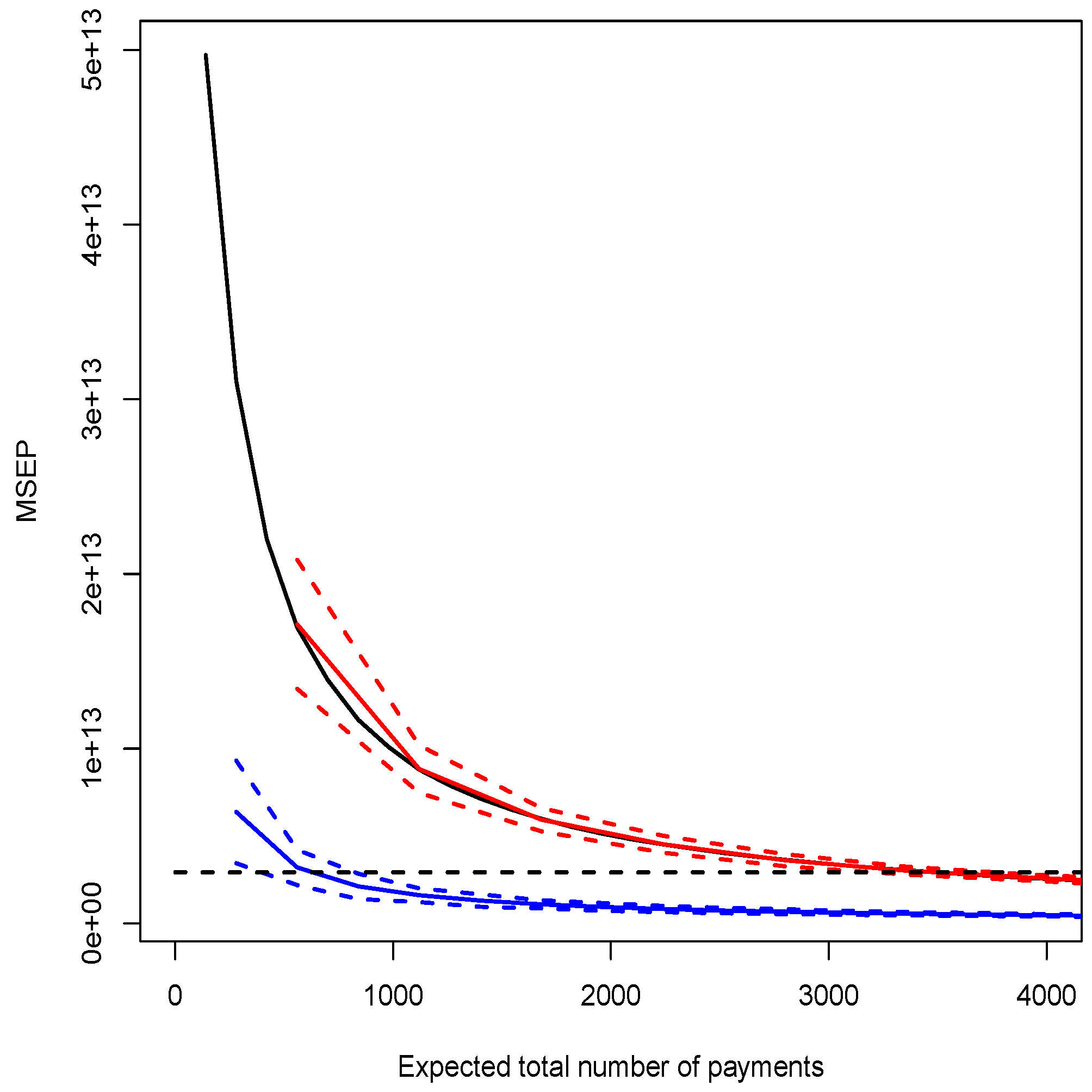
For each value of θ, we repeat this procedure 1000 times and we calculate the average best estimate and the average MSEP. Results are presented in

Table 3. Results.

Method	$\mathbb{E}\left[\mathbf{Reserve}\right]$	$\sqrt{\mathit{MSEP}}$
Mack’s model	28655773	1417267
Poisson reg.
Model A	28655773	11622
Model C	28655773	11622
quasi-Poisson reg.
Model B	28655773	1708196
Model D	28655773	see Figure 1
quasi-Poisson reg.
Model E ($\rho \approx 0$)	28657364	see Figure 2
Model F ($\rho \approx 0.8$)	20514566	see Figure 2

and Figure 1. For Poisson regression (Model A and C), results are similar, which is consistent with Corollary 4. For micro-level models, convergence of $\sqrt{MSEP}$ towards (11622) is fast. For quasi-Poisson regression (Model B and D), expected values are equal and Figure 1 shows $\sqrt{MSEP}$ as a function of the expected total number of payments for the portfolio. Above a certain level, (close to 3400 here), accuracy of the “micro” approach exceeds the “macro”. Again, those results are consistent with Corollary 5. Here, we consider that the expected number of payments by cluster $(\theta$) is constant but it would also be possible to consider a mixture model where $\left(N_g|{\Theta }_g\right)\sim \mathcal{P}\left({\theta }_g\right)$, $g=1,\dots ,m$, and ${\Theta }_g\sim \text{Gamma}(\alpha ,\beta )$. This modification does not change the conclusions. Finally, a comparison of estimated MSEP for both Poisson and quasi-Poisson models confirms the presence of over-dispersion in the data.

In order to illustrate the impact of adding a covariate at the micro-level, we define a quasi-Poisson micro-level model with a weakly correlated covariate (Model E) and with a strongly correlated covariate (Model F). Following a similar procedure, we obtain results presented in the bottom part of Table 3 and in Figure 2.

As opposed to standard classical results on hierarchical models, the average of explanatory variable within a cluster ($(1/n_g){\sum }_i{x}_{ig}$) has not been added to the macro-level model (Model B), for several reasons,

(i)

impossible to compute that average without individual data;

(ii)

discrete explanatory variables used in the micro-level model; and

(iii)

since claims reserve model have a predictive motivation, it is risky to project the value of an aggregated variable on future clusters.

With an explanatory variable highly correlated with the response variable, results obtained with Model D and E are very close. As claimed by Proposition 6 and Equation (14), an explanatory variable highly correlated with the response variable will decrease the value of $\sqrt{MSEP}$, and lowers the threshold above which the micro-level model is more accurate than the macro-level one.

The quasi-Poisson macro-level model (Model B) with maximum likelihood estimators leads to the same reserves as the chain-ladder algorithm and the Mack’s model (see [31]), assuming the clusters exposure, for $(i,j)\in \mathcal{K}$, is one. To obtain similar results with a quasi-Poisson micro-level model (Model D), a similar assumption is necessary: exposure of each claim within cluster $(i,j)$ is $1/n_{i,j}$. That assumption implies, on a micro level, that predicted individual payments ${\widehat{Y}}_{ij}^{\left(k\right)}$ are proportional to $1/n_{ij}$. That assumption has unfortunately no foundation.

In the Poisson and quasi-Poisson micro-level models (Model C and D), payments related to the same claim, in two different clusters are supposed to be non-correlated. As discussed in the previous Section, it is possible to include dependencies among payments for a given claim using a Poisson regression with random effects.

3.2. The Mixed Poisson Model for Reserves

3.2.1. Construction

From the results obtained in Subsection 2.3, it is possible to construct a micro-model for the reserves that includes a random intercept. The later will allow to model dependence between payments from a given claim. Note that it is not relevant to construct an aggregated model with random effects that could be compared with individual ones. In the context of claims reserves, $Y_g^{\left(t\right)}$ represents the sum of payments made for claim t within cluster g. The assumptions of that model (called model G) are

$$\begin{array}{cc}\hfill \left(Y_g^{\left(t\right)}|{\gamma }_t\right)& \sim \mathcal{P}\left({\lambda }_g{e}^{{\gamma }_t}\right),{\lambda }_g=exp[{\mathit{x}}_g^{\mathsf{T}}\mathit{c}+ln(1/n_g)]\hfill \\ \hfill {\gamma }_t& \sim N(0,{\sigma }^2)\hfill \end{array}$$

Because of the hierarchical structure of the model, predictions can be derived from several philosophical perspectives (see [32], and references therein). In our example, we focus on the following unconditional predictions

$$\begin{array}{cc}\hfill \left({\widehat{Y}}_g^{\left(t\right)}|{\gamma }_t\right)& \sim \mathcal{P}\left({\widehat{\lambda }}_g{e}^{{\gamma }_t}\right)\hfill \\ \hfill {\widehat{\lambda }}_g& =exp[{\mathit{x}}_g^{\mathsf{T}}\widehat{\mathit{c}}+ln(1/n_g)]\hfill \\ \hfill \text{so}\text{that}\mathbb{E}\left[{\widehat{Y}}_g^{\left(t\right)}\right]& ={\lambda }_g{e}^{{\sigma }^2/2}\hfill \end{array}$$

and on the conditional ones, where the unknown component of claim t is predicted by the so-called best linear estimate (that minimizes the MSEP) ${\tilde{\gamma }}_t$ (see [25])

$$\begin{array}{cc}\hfill \left({\tilde{Y}}_g^{\left(t\right)}|{\tilde{\gamma }}_t\right)& \sim \mathcal{P}\left({\widehat{\lambda }}_g{e}^{{\tilde{\gamma }}_t}\right)\hfill \\ \hfill \text{so}\text{that}\mathbb{E}\left[{\tilde{Y}}_g^{\left(t\right)}\right]& ={\lambda }_g{e}^{{\tilde{\gamma }}_t}\hfill \end{array}$$

It is then possible to compute the overall best estimate for the total amount of reserves.

3.2.2. Illustration and Discussion

We illustrate these results with the same macro-level dataset. In order to construct a micro-level model from Table 2, we follow a procedure similar to the one described in the previous section,

1-3.

see previous section;

4.

for each accident year, allocate randomly the source (t) of each payment;

5.

fit model G; and

6.

compute the best estimate and the MSEP of the reserve.

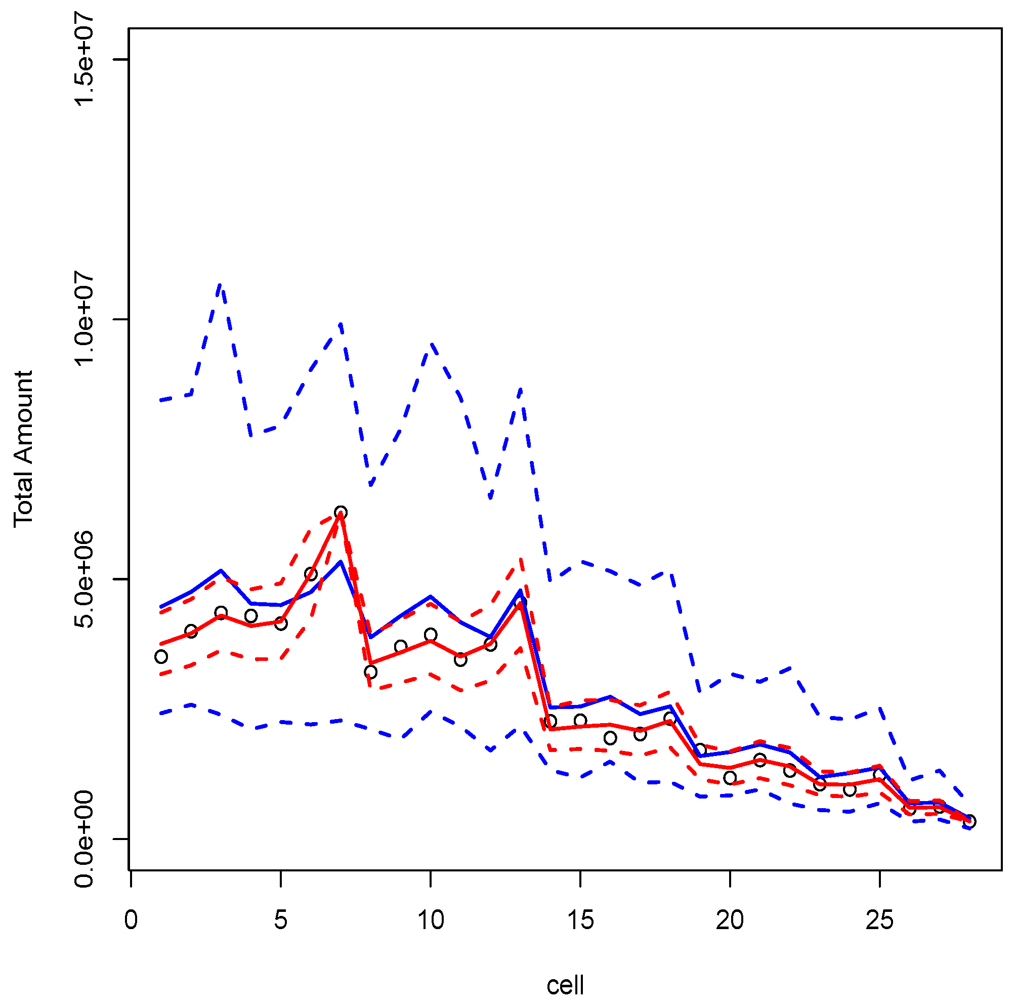
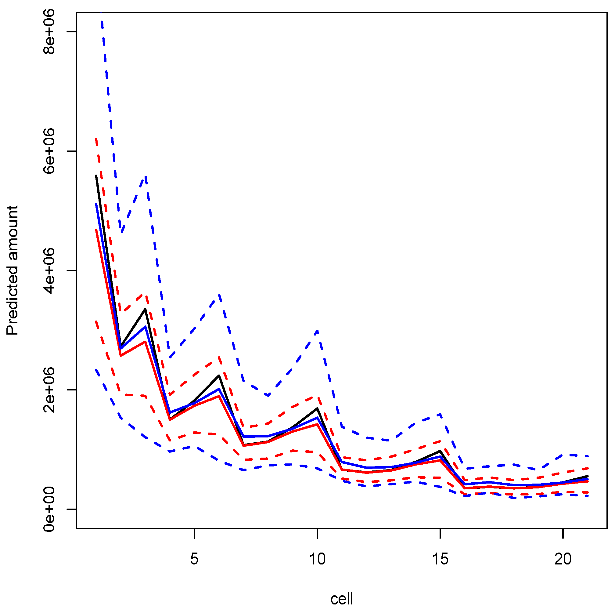
For a fixed value of θ, the procedure is repeated 1000 times. Various values were considered for θ (10, 25, 50, 100 and 250), and results were similar. In order to avoid heavy tables, only the case where $\theta =10$ is mentioned here. Simulations and computations were performed with R, relying on package lme4. Final results are reported in

Table 4. Numerical results for $\theta =10$. Results for different values of θ are similar.

Modèle	$\mathbb{E}\left[\mathbf{Reserve}\right]$	$\sqrt{\mathrm{Var}\left(\mathrm{Reserve}\right)}$
coll. quasi-Pois.	28656423	1708216
mixed Poisson non-cond.	27930624	3297401
mixed Poisson cond.	25972947	2280902

. On Figure 3 we can see predictions of the model on observed data, while on Figure 4 we can see predictions of the model for non-observed cells (with $\pm 2\sigma$ in both cases). For each simulation, a LRT is performed to check the non-nullity of the variance term and to confirm the necessity of including a random intercept in the model, which means that correlation among payments (related to the same claim) is positive. Observe that with the mixed model, the log-likelihood is approximated using numerical integration, which might bias p-values of the test. To avoid that, p have been confirmed using a bootstrap procedure (using package glmmML).

4. Conclusions

In this article, we study equivalence (as well as non-equivalence) between Poisson and quasi-Poisson regression models, obtained on aggregated (so called macro-level) and non-aggregated (micro-level) datasets, in order to understand when using micro-level models might over-perform macro-level ones. Those models are used here in the context of estimating claims reserves. The uncertainty is quantified using—as in standard macro-level approaches—the MSEP. We also investigate the impact of adding micro-level covariates in the model. Finally, we discuss the use of mixed Poisson regression, in the case of micro-level data, that might take into account possible dependence between observations in different clusters.

We illustrate theoretical results on simulated data, generated from cumulated payments, in R. A methodology that allows us to generate such micro-level datasets is described. In a first part, we compare results obtained with Poisson and quasi-Poisson regression, on micro- and macro-level datasets. That comparison reveals that in the context of a quasi-Poisson regression model, the expected number of claims plays a crucial role, since above a given threshold, the micro-level model is more robust than the macro-one. Moreover, the presence (or absence) of covariates can affect this threshold.

In a second part, we analyse predictions obtained using a mixed Poisson regression model, i.e., a Poisson regression model with a random component that characterizes dependence among payments on the same claim, at different dates. The necessity of this random component is verified by using a likelihood-ratio test. That study reveals that such a dependence might have a non-negligible impact on predictions.

Of course, that study is only the first step and several directions for future research can be intuited. For instance, as micro-level models are based on much more observations than macro-level ones, more robust estimation techniques, such as generalized method of moments, can be considered.

References

1. E. Astesan. Les réserves techniques des sociétés d’assurances contre les accidents automobiles. Paris, France: Librairie générale de droit et de jurisprudence, 1938. [Google Scholar]
2. R. Mack. “Distribution-free calculation of the standard error of chain ladder reserve estimates.” ASTIN Bull. 23 (1993): 213–225. [Google Scholar] [CrossRef]
3. P.D. England, and R.J. Verrall. “Stochastic claims reserving in general insurance.” Br. Actuar. J. 8 (2003): 443–518. [Google Scholar] [CrossRef]
4. J. Van Eeghen. “Loss reserving methods.” In Surveys of Actuarial Studies 1. The Hague, The Netherlands: Nationale-Nederlanden, 1981. [Google Scholar]
5. G.C. Taylor. Claims Reserving in Non-Life Insurance. Amsterdam, The Netherlands: North-Holland, 1986. [Google Scholar]
6. J.E. Karlsson. “The expected value of IBNR claims.” Scand. Actuar. J. 1976 (1976): 108–110. [Google Scholar] [CrossRef]
7. E. Arjas. “The claims reserving problem in nonlife insurance—Some structural ideas.” ASTIN Bull. 19 (1989): 139–152. [Google Scholar] [CrossRef]
8. W.S. Jewell. “Predicting IBNYR events and delays I. Continuous time.” ASTIN Bull. 19 (1989): 25–55. [Google Scholar] [CrossRef]
9. R. Norberg. “Prediction of outstanding liabilities in non-life insurance.” ASTIN Bull. 23 (1993): 95–115. [Google Scholar] [CrossRef]
10. O. Hesselager. “A Markov model for loss reserving.” ASTIN Bull. 24 (1994): 183–193. [Google Scholar] [CrossRef]
11. R. Norberg. “Prediction of outstanding liabilities II: Model variations and extensions.” ASTIN Bull. 29 (1999): 5–25. [Google Scholar] [CrossRef]
12. O. Hesselager, and R.J. Verrall. “Reserving in Non-Life Insurance.” Available online: http://onlinelibrary.wiley.com (accesssed on 29 February 2016).
13. X.B. Zhao, X. Zhou, and J.L. Wang. “Semiparametric model for prediction of individual claim loss reserving.” Insur. Math. Econ. 45 (2009): 1–8. [Google Scholar] [CrossRef]
14. X. Zhao, and X. Zhou. “Applying copula models to individual claim loss reserving methods.” Insur. Math. Econ. 46 (2010): 290–299. [Google Scholar] [CrossRef]
15. M. Pigeon, K. Antonio, and M. Denuit. “Individual loss reserving using paid-incurred data.” Insur. Math. Econ. 58 (2014): 121–131. [Google Scholar] [CrossRef]
16. K. Antonio, and R. Plat. “Micro-level stochastic loss reserving for general insurance.” Scand. Actuar. J. 2014 (2014): 649–669. [Google Scholar] [CrossRef]
17. X. Jin, and E.W. Frees. “Comparing Micro- and Macro-Level Loss Reserving Models.” Madison, WI, USA: Presentation at ARIA, 2015. [Google Scholar]
18. A. Johansson. “Claims Reserving on Macro- and Micro-Level.” Master’s Thesis, Royal Institute of Technology, Stockholm, Sweden, 2015. [Google Scholar]
19. J. Friedland. Estimating Unpaid Claims Using Basic Techniques. Arlington, VA, USA: Casualty Actuarial Society, 2010. [Google Scholar]
20. G.J. Van den Berga, and B. van der Klaauw. “Combining micro and macro unemployment duration data.” J. Econom. 102 (2001): 271–309. [Google Scholar] [CrossRef]
21. F. Altissimo, B. Mojon, and P. Zaffaroni. Fast Micro and Slow Macro: Can Aggregation Explain the Persistence of Inflation? European Central Bank Working Papers; 2007, Volume 0729. [Google Scholar]
22. W.H. Greene. Econometric Analysis, 5th ed. Upper Saddle River, NJ, USA: Prentice Hall, 2003. [Google Scholar]
23. P. McCullagh, and J.A. Nelder. Generalized Linear Models. London, UK: Chapman & Hall, 1989. [Google Scholar]
24. G.M. Cordeiro, and P. McCullagh. “Bias correction in generalized linear models.” J. R. Stat. Soc. B 53 (1991): 629–643. [Google Scholar]
25. M. Wüthrich, and M. Merz. Stochastic Claims Reserving Methods. Hoboken, NJ, USA: Wiley Interscience, 2008. [Google Scholar]
26. M. Ruoyan. “Estimation of Dispersion Parameters in GLMs with and without Random Effects.” Stockholm University, 2004. Available online: http://www2.math.su.se/matstat/reports/serieb/2004/rep5/report.pdf (accessed on 29 February 2016).
27. T.A.B. Snijders, and R.J. Bosker. Multilevel Analysis: An Introduction to Basic and Advanced Multilevel Modeling. Thousand Oaks, CA, USA: Sage Publishing, 2012. [Google Scholar]
28. S.G. Self, and K.Y. Liang. “Asymptotic properties of maximum likelihood estimators and likelihood ratio tests under nonstandard conditions.” J. Am. Stat. Assoc. 82 (1987): 605–610. [Google Scholar] [CrossRef]
29. D. Dunson. Random Effect and Latent Variable Model Selection. Lecture Notes in Statistics; New York, NY, USA: Springer-Verlag, 2008, Volume 192. [Google Scholar]
30. S. Christofides. “Regression models based on log-incremental payments.” Claims Reserv. Man. 2 (1997): D5.1–D5.53. [Google Scholar]
31. T. Mack, and G. Venter. “A comparison of stochastic models that reproduce chain ladder reserve estimates.” Insur. Math. Econ. 26 (2000): 101–107. [Google Scholar] [CrossRef]
32. A. Skrondal, and S. Rabe-Hesketh. “Prediction in multilevel generalized linear models.” J. R. Stat. Soc. A 172 (2009): 659–687. [Google Scholar] [CrossRef]
Figure 1. Square root of the mean square error of prediction obtained for Model D (solid line) and Model B (broken line) from simulated values for increasing expected number of payments for the portfolio.
Risks 04 00012 g001
Figure 2. Mean square error of prediction ( ± 2 σ ) obtained from simulated values as a function of the expected number of payments for Model E (red lines) and Model F (blue lines). For comparison purposes, the MSEP obtained for the Model D (solid black line) and the Model B (broken black line) are added.
Risks 04 00012 g002
Figure 3. Observed data (circles) with conditional predictions (red lines) and unconditional ones (blue lines) from Model G with θ = 10 .
Risks 04 00012 g003
Figure 4. Predictions with the quasi-Poisson macro-level model (strong black line), with conditional predictions (red lines) and unconditional ones (blue lines) from Model G with θ = 10 .
Risks 04 00012 g004