Environmental Constraints in Cryptocurrency Portfolio Optimization: A Mean-CVaR Analysis

Abstract

Sustainable investing raises an important question: do environmental restrictions affect the risk–return characteristics of cryptocurrency portfolios? This study compares Mean-CVaR optimal portfolios across Green, Dirty, and Mixed cryptocurrency universes using daily returns for 12 cryptocurrencies from January 2022 to September 2025. Ethereum (ETH) was classified as Dirty before its transition from Proof-of-Work to Proof-of-Stake in September 2022 and as Green thereafter. Each universe is optimized independently using the Non-Dominated Sorting Genetic Algorithm II (NSGA-II), Strength Pareto Evolutionary Algorithm 2 (SPEA2), and Particle Swarm Optimization (PSO), with CVaR measured at the 95% confidence level. The results show that, in the Post-Merge period, the Green universe exhibits a higher CVaR than the Dirty and Mixed universes under all three algorithms. This result remains consistent across the main robustness analyses and is confirmed by an exact optimization benchmark. The asset-exclusion analysis further shows that excluding Bitcoin (BTC) increases CVaR under all three algorithms, whereas excluding ETH does not produce the same effect. These findings indicate that environmental screening can alter portfolio risk by changing the assets available for investment. For sustainability-oriented investors, the financial effect of such restrictions therefore depends on the assets excluded from the portfolio.

1. Introduction

Cryptocurrency portfolio management has attracted increasing academic and practical interest in recent years. Cryptocurrencies are no longer a marginal segment of the financial market. They are now held by individual investors, trading platforms, funds, and, increasingly, institutions that manage diversified portfolios. Consequently, risk management has become a practical concern. Recent market conditions have reinforced this concern. The COVID-19 pandemic, the Russia–Ukraine conflict, and the escalation of geopolitical tensions in the Middle East have created uncertainty, liquidity pressure, and sharp price movements in digital assets. During these episodes, cryptocurrencies sometimes moved with traditional financial markets before diverging from them. This behavior suggests that the asset class is exposed to both market-wide shocks and asset-specific dynamics. For investors, the main concern is not only volatility during normal periods. A single extreme loss can offset the gains accumulated over a long period. Therefore, controlling tail losses is central when cryptocurrencies are included in investment portfolios.

In addition, the growth of cryptocurrency investment has intensified concerns regarding environmental sustainability. The energy demand of Proof-of-Work mining, especially Bitcoin (BTC) mining, has raised questions about the sustainability of some digital assets. BTC mining alone has been estimated to consume approximately 130 TWh of electricity per year, which is comparable to the electricity demand of a midsized economy. In contrast, low-energy consensus mechanisms, such as Proof-of-Stake, require far less energy. For example, the 2022 transition of Ethereum (ETH) to Proof-of-Stake reduced its energy use by more than 99%. These differences have led researchers and investors to distinguish between energy-intensive “Dirty” cryptocurrencies and low-energy “Green” cryptocurrencies (Ali et al. 2024; Pham et al. 2022). Although this distinction has ethical dimensions, it also has direct portfolio implications. As sustainable finance rules and ESG mandates become more influential, some investors may be unable or unwilling to hold energy-intensive assets. Therefore, a Green-only cryptocurrency portfolio is a realistic investment case, and its risk–return properties require direct examination.

Ideally, sustainable investors can reduce environmental exposure without losing tail-risk efficiency. A portfolio restricted to Green cryptocurrencies would provide diversification, limit extreme losses, and remain competitive with portfolios that include energy-intensive assets. However, portfolio optimization may not support this ideal outcome. Low dependence between assets does not necessarily imply that they will receive positive weights in an optimized portfolio. If an excluded Dirty asset has a stronger tail-risk profile than the available Green alternatives, environmental restrictions may create a measurable risk–return cost. Therefore, it remains unclear whether the diversification benefits attributed to Green cryptocurrencies persist when Green and Dirty assets compete directly for portfolio weight under a common tail-risk objective.

This question also requires a risk measure that is suited to cryptocurrency returns. The classical mean-variance model proposed by Markowitz (1952) remains the foundation of portfolio theory, but its assumptions are restrictive for digital asset portfolios. Cryptocurrency returns are often asymmetric, heavy-tailed, and subject to sudden jumps. Variance treats upside and downside movements in the same way, whereas investors are mainly concerned with losses. VaR provides a loss threshold but does not measure the expected severity of losses beyond that threshold and may violate subadditivity. In contrast, Conditional Value-at-Risk (CVaR) measures the expected loss in the tail of the distribution and satisfies the coherence properties required for a sound risk measure (Artzner et al. 1999; Rockafellar and Uryasev 2000). Because investors seek to minimize CVaR and maximize expected returns simultaneously, the portfolio problem is naturally bi-objective. Population-based algorithms, such as NSGA-II, SPEA2, and PSO, are useful in this setting because they can approximate a set of efficient portfolios rather than solving only one weighted objective (Deb et al. 2002; Xu et al. 2007; Zitzler et al. 2001).

The existing literature provides useful evidence but does not fully resolve the allocation problem. Several studies have reported that Green cryptocurrencies offer diversification benefits or protection against downside risk (Ali et al. 2024; Naeem et al. 2023; Pham et al. 2022). These studies are valuable because they examine dependence, co-movement, spillovers, and tail relationships between Green cryptocurrencies and other assets. However, much of this research focuses on co-movement rather than optimized portfolio weights. Dependence is not an allocation. An asset can have a low correlation with another asset and still receive little or no weight when the portfolio is optimized under a specific objective. In addition, a second strand of research shows that energy-intensive cryptocurrencies can transmit return and volatility shocks (Duan et al. 2023; Umar et al. 2022). A third strand examines cryptocurrency allocation more directly and finds that BTC and ETH often dominate optimized portfolios (Bakry et al. 2021; Ma et al. 2020; Som and Kayal 2022). However, these strands remain only partially connected.

A related methodological issue is the role of the optimizer. Evolutionary algorithms have been used in portfolio optimization and, in some cases, in cryptocurrency allocation (Guarino et al. 2024; Kaucic et al. 2019; Mba and Mai 2022). To date, however, there has been limited systematic analysis of whether environmentally defined cryptocurrency universes produce stable allocation results under different population-based solvers. This is important because an allocation may reflect the structure of the data, but it may also reflect the behavior of a particular algorithm. The comparison of several solvers helps to separate these two possibilities. If the same universe-level result appears under NSGA-II, SPEA2, and PSO, the finding is less likely to be specific to one optimization method.

This study addresses these gaps by comparing three cryptocurrency universes: Green, Dirty, and Mixed. The Green universe contains low-energy cryptocurrencies, the Dirty universe contains energy-intensive cryptocurrencies, and the Mixed universe combines both groups. All three universes are optimized under the same Mean-CVaR objective using daily returns for 12 cryptocurrencies from January 2022 to September 2025. Because ETH transitioned from Proof-of-Work to Proof-of-Stake in September 2022, its environmental classification changes between the Pre-Merge and Post-Merge periods. Each portfolio problem is solved independently using NSGA-II, SPEA2, and PSO.

This study has three objectives. First, it examines whether an environmental restriction changes the efficient frontier and the resulting optimal allocation. Second, it compares the return and tail risk of Green, Dirty, and Mixed cryptocurrency portfolios. Third, it assesses whether this comparison is stable across three independent population-based solvers. These objectives make it possible to examine not only whether Green portfolios differ from Dirty and Mixed portfolios but also whether the difference depends on the algorithm used.

This study contributes to the literature in two main ways. First, it moves beyond dependence-based evidence and examines Green and Dirty cryptocurrencies through direct portfolio optimization. It assesses how environmental restrictions affect portfolio allocation under a common Mean-CVaR objective. Second, it compares the same portfolio problem across three population-based algorithms, providing evidence on the consistency of the results across optimization methods. For practice, this study provides information on the risk implications of restricting the cryptocurrency investment universe on environmental grounds.

The results show that environmental restrictions affect the risk–return characteristics of cryptocurrency portfolios. The main findings are consistent across the three optimization algorithms and remain stable under additional robustness analyses. The results also show that the effect of the restriction depends on the composition of the investment universe and should not be interpreted as evidence that Green cryptocurrencies are inherently riskier.

The remainder of this paper is organized as follows. Section 2 reviews the relevant literature. Section 3 presents the data, models, and algorithms used in this study. Section 4 reports the empirical and robustness results. Section 5 discusses the findings, and Section 6 concludes the paper.

2. Literature Review

A large body of literature has examined cryptocurrency portfolio optimization from different perspectives. Three areas are most relevant to this study. The first concerns the choice of risk measure, especially the move from variance and Value-at-Risk to coherent tail-risk measures such as Conditional Value-at-Risk (CVaR). The second examines whether environmentally classified cryptocurrencies differ in their financial behavior and portfolio roles. The third applies evolutionary algorithms to multi-objective portfolio optimization. Each area provides useful evidence for the study. However, these areas are not fully connected. What remains unclear is whether the Green, Dirty, and Mixed cryptocurrency universes behave differently when they are optimized under the same Mean-CVaR objective. This section reviews these areas and identifies the gaps addressed in this study.

2.1. From Mean-Variance to Coherent Tail-Risk Measures

Modern portfolio theory begins with the mean-variance framework proposed by Markowitz (1952). This framework formalizes the risk–return trade-off and introduces the efficient frontier as a basis for portfolio selection. It remains central to finance, but its assumptions are restrictive for cryptocurrency markets. Mean-variance optimization treats gains and losses symmetrically and works best when returns are close to normality. Cryptocurrency returns often violate these assumptions because they are volatile, asymmetric, and heavy-tailed. Therefore, a risk measure focused on extreme losses is more suitable for this asset class.

The limitations of Value-at-Risk (VaR) further support the use of CVaR. Artzner et al. (1997, 1999) show that VaR may violate subadditivity and therefore does not satisfy the axioms of a coherent risk measure. VaR identifies a loss threshold but does not measure the expected size of losses beyond that threshold. CVaR addresses this weakness by measuring the expected loss in the tail of the return distribution. Rockafellar and Uryasev (2000) made CVaR useful for portfolio optimization by reformulating its minimization as a tractable programming problem. Yamai and Yoshiba (2002) and Krokhmal et al. (2002) further show that CVaR is more informative than VaR for risk decomposition and portfolio optimization when losses are extreme or return distributions depart from normality.

Previous research has also improved the estimation of tail risk under non-Gaussian returns. Early work combined GARCH models, Extreme Value Theory, and copulas to capture volatility clustering, heavy tails, and nonlinear dependence (Boubaker and Sghaier 2013; Hotta et al. 2008). Later studies extended this approach by integrating vine copulas with GARCH-EVT-CVaR frameworks and reported improvements in tail-risk estimation across financial markets (Sahamkhadam et al. 2018). Similarly, Khaki et al. (2022) show that higher-moment models can outperform mean-variance optimization when returns are non-normal.

These studies establish two points relevant to the present study. First, CVaR is more appropriate than variance for assets with heavy-tailed returns. Second, tail-risk modeling should account for non-normality, especially in cryptocurrency markets. However, much of this literature focuses on risk measurement or risk estimation rather than optimized allocation. It does not examine how environmentally classified cryptocurrencies compete for portfolio weights when the optimization criterion is Mean-CVaR. Therefore, these studies justify the use of CVaR, but they do not answer the allocation question addressed in this study.

2.2. Cryptocurrencies in Portfolios: The Green-Dirty Divide

The environmental cost of cryptocurrency mining has created a distinction between energy-intensive or “Dirty” cryptocurrencies and low-energy or “Green” alternatives. This distinction is important for sustainable finance because some investors may face ESG mandates or internal environmental restrictions. Therefore, the relevant question is not only whether Green and Dirty cryptocurrencies differ but also whether this difference affects optimized portfolio allocation.

Environmental considerations have also been incorporated into quantitative decision-making frameworks in the broader energy and carbon literature. Liu et al. (2023) model the timing of carbon emission right purchases as an optimal stopping problem, providing a quantitative approach to environmental asset management. More recently, Liu et al. (2026) develop a multi-source framework for monitoring and certifying carbon emissions in carbon-neutral industrial parks. Although these studies address different settings, they illustrate the increasing role of quantitative methods in environmental decision-making and measurement. This study examines this issue in cryptocurrency portfolios by incorporating environmental classification directly into the investment universe.

The existing literature on Green and Dirty cryptocurrencies has identified several differences in their financial behavior. On the Dirty side, Umar et al. (2022) identify energy-intensive cryptocurrencies as important transmitters of return and volatility shocks. Duan et al. (2023) show that Dirty cryptocurrencies maintain stronger links with traditional financial markets than Green cryptocurrencies, especially during periods of economic stress. These findings suggest that Dirty assets may play an important role in the transmission of shocks. However, they do not show whether such assets should receive high or low portfolio weights under a tail-risk objective.

The evidence on the portfolio role of Green cryptocurrencies is not uniform. Pham et al. (2022) report low correlations between Green and non-Green cryptocurrencies, while Naeem et al. (2023) find that selected Green cryptocurrencies may provide protection against extreme losses. In contrast, Ali et al. (2024) document return and volatility spillovers between Green cryptocurrencies and G7 equity markets, while Duan et al. (2023) show that the connections between clean and Dirty cryptocurrencies and financial assets vary with economic policy uncertainty. Together, these findings indicate that the portfolio role of Green cryptocurrencies can differ across markets and under different conditions.

However, these studies primarily focus on correlations, spillovers, dependence, or downside-risk transmission. These analyses describe the relationships among asset returns, but they do not determine the portfolio weights selected when expected return and CVaR are optimized jointly. An asset may provide diversification benefits and still receive little or no weight in an optimal portfolio if other assets offer a better risk–return combination. This distinction is particularly important for environmentally constrained investors because screening changes the set of assets available for portfolio allocation.

Additional research investigates portfolio allocation. Ma et al. (2020) and Som and Kayal (2022) indicate that incorporating BTC can affect portfolio performance. Furthermore, Bakry et al. (2021) demonstrate that the optimal portfolio weight of BTC is sensitive to investment constraints. These studies determine portfolio allocations directly but do not systematically distinguish cryptocurrencies according to environmental classification.

Therefore, a gap exists between these two strands of research. Studies on Green and Dirty cryptocurrencies mainly provide evidence of co-movement, spillovers, and diversification, whereas allocation studies compute portfolio weights without explicitly examining environmental screening. The present study connects these two areas by optimizing Green, Dirty, and Mixed cryptocurrency universes under the same Mean-CVaR objective and comparing the resulting allocations across NSGA-II, SPEA2, and PSO.

2.3. Evolutionary Algorithms for Multi-Objective Portfolio Optimization

The Mean-CVaR portfolio problem inherently presents a bi-objective challenge, as investors aim to maximize expected returns while minimizing tail risk. Evolutionary algorithms are useful in this setting because they can approximate a set of Pareto-efficient solutions without reducing the problem to a single weighted objective. This feature is especially relevant when the aim is not only to obtain one portfolio but also to examine how different asset universes shape the efficient frontier.

Several studies have applied evolutionary algorithms to downside-risk portfolio optimization. Kaucic et al. (2019) were among the first to adapt NSGA-II and SPEA2 to semivariance and CVaR objectives. Their study supports the use of evolutionary algorithms when the risk measure captures downside risk rather than variance alone. In cryptocurrency markets, Mba and Mai (2022) combine copula modeling with particle swarm optimization to improve portfolio performance under extreme market conditions, whereas Bedoui et al. (2023) extend evolutionary optimization to portfolios that combine cryptocurrencies with conventional financial assets.

More recent studies have developed this field in different directions. Ghanbari et al. (2024) proposed a credibilistic Mean-CVaR framework in which cryptocurrency returns are modeled through fuzzy variables. Their model also includes practical constraints, such as cardinality and floor–ceiling limits. This study improves the treatment of uncertainty and investment restrictions in cryptocurrency portfolio construction. However, it does not examine whether environmental classification changes the optimal allocation of resources. In a different setting, Abdallah et al. (2025) compare NSGA-II, SPEA2, and PSO within a Mean-CVaR framework using equities, commodities, Green bonds, and two cryptocurrencies. Their results show that portfolio composition may vary across optimization algorithms and market regimes. However, cryptocurrencies represent only a small part of the investment universe, and the study does not distinguish between Green and Dirty digital assets.

The literature shows that evolutionary algorithms are suitable for multi-objective portfolio optimization and that algorithm choice can affect portfolio composition. However, it does not fully address the problem examined in this study. Existing studies tend to focus on uncertainty modeling, algorithm comparisons, or broad asset portfolios. To the best of our knowledge, no study has jointly examined whether environmental classification affects cryptocurrency portfolio allocation when Green, Dirty, and Mixed universes are optimized under the same Mean-CVaR objective and compared across several population-based solvers.

Therefore, the existing literature reveals a clear research gap. CVaR provides a tail-risk criterion, while the Green-Dirty distinction defines the investment universe. NSGA-II, SPEA2, and PSO provide independent optimization procedures to assess the consistency of the allocation results. The present study brings these elements together in a common empirical framework.

Using three independent optimization methods is important because the main question concerns differences between investment universes rather than the performance of a single algorithm. Consistent universe-level results across NSGA-II, SPEA2, and PSO therefore provide evidence that the observed comparison is not specific to a single optimization procedure.

The following section presents the data, the Mean-CVaR model, and the optimization algorithms used in the empirical analysis.

3. Materials and Methods

3.1. Data

The empirical analysis uses daily price data for 12 cryptocurrencies: BTC, Bitcoin Cash (BCH), Litecoin (LTC), Monero (XMR), Ethereum Classic (ETC), Dogecoin (DOGE), ETH, Cardano (ADA), Solana (SOL), Algorand (ALGO), Tezos (XTZ), and Nano (XNO). The data were obtained from Yahoo Finance and cover the period from January 2022 to September 2025.

Cryptocurrencies are classified according to their consensus mechanisms. BTC, BCH, LTC, XMR, ETC, and DOGE are treated as energy-intensive assets, while ADA, SOL, ALGO, XTZ, and XNO are treated as low-energy assets. ETH changed from Proof-of-Work to Proof-of-Stake on 15 September 2022 (Kapengut and Mizrach 2023). Accordingly, ETH is classified as Dirty before the transition and as Green thereafter. The sample is divided into a Pre-Merge period from January 2022 to 14 September 2022 and a Post-Merge period from 16 September 2022 to September 2025. The transition date, 15 September 2022, is excluded from both periods to avoid ambiguity in the environmental classification on the day of the Merge.

Table 1. Consensus mechanisms and environmental classification of the selected cryptocurrencies.

Asset	Consensus Mechanism	Pre-Merge	Post-Merge
BTC	Proof-of-Work (PoW)	Dirty	Dirty
BCH	Proof-of-Work (PoW)	Dirty	Dirty
LTC	Proof-of-Work (PoW)	Dirty	Dirty
XMR	Proof-of-Work (PoW)	Dirty	Dirty
ETC	Proof-of-Work (PoW)	Dirty	Dirty
DOGE	Proof-of-Work (PoW)	Dirty	Dirty
ETH	PoW/Proof-of-Stake (PoS)	Dirty	Green
ADA	Proof-of-Stake (PoS)	Green	Green
SOL	Proof-of-Stake (PoS)	Green	Green
ALGO	Pure Proof-of-Stake (PPoS)	Green	Green
XTZ	Proof-of-Stake (PoS)	Green	Green
XNO	Open Representative Voting	Green	Green

Note: The environmental classification is based on the energy requirements of the consensus mechanism. Proof-of-Work cryptocurrencies are classified as energy-intensive, while cryptocurrencies using non-mining, low-energy consensus mechanisms are classified as Green. ETH transitioned from Proof-of-Work to Proof-of-Stake on 15 September 2022; its energy consumption declined by more than 99% following this transition.

summarizes the consensus mechanisms and period-specific environmental classification of the selected cryptocurrencies.

In the Pre-Merge period, the Green universe contains ADA, SOL, ALGO, XTZ, and XNO, while the Dirty universe contains BTC, BCH, LTC, XMR, ETC, DOGE, and ETH. In the Post-Merge period, ETH enters the Green universe, which contains ETH, ADA, SOL, ALGO, XTZ, and XNO, while the Dirty universe contains BTC, BCH, LTC, XMR, ETC, and DOGE. The Mixed universe contains all 12 cryptocurrencies in both periods.

The selected cryptocurrencies provide a common empirical sample of energy-intensive and low-energy assets with clearly identifiable consensus mechanisms and daily price data available over the study period. Using the same observation window allows the three investment universes to be compared with a consistent data structure.

Daily prices are transformed into continuously compounded returns as

$$R_t=\ln \left(P_t\right)-\ln \left(P_{t-1}\right),$$

(1)

where $R_t$ denotes the return at time t, $P_t$ is the price at time t, and $P_{t-1}$ is the price on the previous trading day. These return series are used for the Mean-CVaR portfolio optimization.

3.2. Mean-CVaR Model

The portfolio optimization problem uses CVaR as the measure of tail risk, which is appropriate for the fat-tailed and non-normal return distributions documented for these assets. For a portfolio loss L at a confidence level $\beta \in (0,1)$, CVaR is the expected loss conditional on the loss exceeding the corresponding VaR (Acerbi and Tasche 2002; Rockafellar and Uryasev 2002).

$${\mathrm{CVaR}}_{\beta }\left(L\right)=\mathbb{E}\left[L\mid L\ge {\mathrm{VaR}}_{\beta }\left(L\right)\right],$$

(2)

where L denotes the portfolio loss. The term ${\mathrm{VaR}}_{\beta }\left(L\right)$ is the Value-at-Risk at level $\beta$, and ${\mathrm{CVaR}}_{\beta }\left(L\right)$ measures the expected loss in the worst $1-\beta$ proportion of outcomes. By construction, ${\mathrm{CVaR}}_{\beta }\left(L\right)\ge {\mathrm{VaR}}_{\beta }\left(L\right)$.

Consider a portfolio of n assets. Let $X={(x_1,\dots ,x_n)}^{\top }$ be the vector of portfolio weights, with $x_i\ge 0$ for all i and ${\sum }_{i=1}^n{x}_i=1$. Let $Y={(y_1,\dots ,y_n)}^{\top }$ be the vector of individual asset returns. The portfolio loss function is

$$f(X,Y)=X^{\top }Y.$$

(3)

Because the direct minimization of (2) is difficult, Rockafellar and Uryasev (2002) introduce a convex and continuously differentiable auxiliary function that transforms CVaR minimization into the minimization of a convex function:

$$F_{\beta }(X,\alpha )=\alpha +{\displaystyle \frac{1}{1-\beta }}{\int }_{Y\in {\mathbb{R}}^n}{\left[f(X,Y)-\alpha \right]}^{+}P\left(Y\right)dY,$$

(4)

where $\alpha \in \mathbb{R}$ is an auxiliary variable, $P\left(Y\right)$ is the probability density of asset returns, and ${\left[u\right]}^{+}=\max (u,0)$. The VaR at level $\beta$ is the value of $\alpha$ that minimizes this function,

$${\mathrm{VaR}}_{\beta }\left(X\right)\in \arg \underset{\alpha \in \mathbb{R}}{\min }{F}_{\beta }(X,\alpha ),$$

(5)

and CVaR is obtained as the corresponding minimum,

$${\mathrm{CVaR}}_{\beta }\left(X\right)=\underset{\alpha \in \mathbb{R}}{\min }{F}_{\beta }(X,\alpha )=F_{\beta }\left(X,{\mathrm{VaR}}_{\beta }\left(X\right)\right).$$

(6)

When the return distribution is not available in closed form, $F_{\beta }(X,\alpha )$ is approximated using a finite set of q return scenarios ${\left\{Y_k\right\}}_{k=1}^q$:

$${\tilde{F}}_{\beta }(X,\alpha )=\alpha +{\displaystyle \frac{1}{q(1-\beta )}}{\displaystyle \sum _{k=1}^q}{\left[X^{\top }{Y}_k-\alpha \right]}^{+}.$$

(7)

In this study, the scenarios ${\left\{Y_k\right\}}_{k=1}^q$ are the observed daily return vectors, so that q equals the number of return observations.

Building on (7), the Mean-CVaR optimization problem replaces variance with CVaR as the risk measure and is expressed as the linear program

$$\begin{array}{ccc}\hfill \underset{X,\alpha ,u}{\min }& \alpha +{\displaystyle \frac{1}{q(1-\beta )}}{\displaystyle \sum _{k=1}^q}{u}_k\hfill & \\ \hfill \mathrm{s}.\mathrm{t}.& X^{\top }{Y}_k+\alpha +u_k\ge 0,\hfill & k=1,\dots ,q,\hfill \\ \hfill & u_k\ge 0,\hfill & k=1,\dots ,q,\hfill \\ \hfill & {\displaystyle \frac{1}{q}}{\displaystyle \sum _{k=1}^q}{X}^{\top }{Y}_k\ge \rho ,\hfill & \\ \hfill & {\displaystyle \sum _{i=1}^n}{x}_i=1,x_i\ge 0,\hfill & i=1,\dots ,n.\hfill \end{array}$$

(8)

where $u_k$ are auxiliary variables representing scenario losses beyond $\alpha$, and $\rho$ is the investor’s minimum required expected return. Varying $\rho$ traces the efficient frontier in the Mean-CVaR space. Apart from the budget and non-negativity constraints in (8), no lower or upper bounds are imposed on individual weights, so the composition of each optimal portfolio is determined entirely by the data.

The CVaR confidence level used in the main empirical analysis is $\beta =95\%$.

3.3. Evolutionary Algorithms

The Mean-CVaR problem in (8) is optimized independently with NSGA-II, SPEA2, and PSO for the Dirty, Green, and Mixed universes. The three algorithms are standard population-based optimizers, and no modifications to their internal operators are introduced. Solving the same problem with three independent algorithms allows the consistency of the resulting allocations across methods to be assessed. Although Equation (8) is convex and can be solved exactly, the three evolutionary algorithms are used because they approximate the entire efficient frontier in a single run.

NSGA-II (Deb et al. 2002) is an elitist genetic algorithm that ranks candidate solutions through fast non-dominated sorting and preserves diversity along the Pareto front using a crowding-distance measure and a crowded comparison operator. In each generation, the parent and offspring populations are merged and ranked by Pareto dominance, and the next population is filled front by front. Within the last admitted front, solutions located in less crowded regions are retained. Offspring are produced by binary tournament selection followed by simulated binary crossover and polynomial mutation.

SPEA2 (Zitzler et al. 2001) maintains an external archive of fixed size that stores the non-dominated solutions found during the search. Each solution receives a fitness value that combines a strength component, derived from the number of solutions it dominates and the number by which it is dominated, with a density component based on the distance to its kth nearest neighbour in the objective space. After the population and archive are merged, the non-dominated solutions are copied to the next archive. If the archive exceeds its capacity, a truncation operator removes the solutions that are closest to one another until the size constraint is satisfied.

PSO (Xu et al. 2007) represents each candidate portfolio as a particle moving through the search space. Consider a swarm of N particles; the position and velocity of particle i are $X_i=(x_{i,1},\dots ,x_{i,n})$ and $V_i=(v_{i,1},\dots ,v_{i,n})$. Each particle records its own best position (local best), while the swarm retains the best position found by any particle (global best). At iteration t, the velocity and position of particle i in dimension j are updated as

$$v_{i,j}^{t+1}=w{v}_{i,j}^t+c_1{\mathrm{rand}}_1\left(p_{i,j}^t-x_{i,j}^t\right)+c_2{\mathrm{rand}}_2\left(p_{g,j}^t-x_{i,j}^t\right),$$

(9)

$$x_{i,j}^{t+1}=x_{i,j}^t+v_{i,j}^t,$$

(10)

for $i=1,\dots ,N$ and $j=1,\dots ,n$, where w is the inertia weight, $c_1$ and $c_2$ are the acceleration coefficients controlling the attraction toward the local best $p_{i,j}$ and the global best $p_{g,j}$, and ${\mathrm{rand}}_1$ and ${\mathrm{rand}}_2$ are independent random numbers drawn from the uniform distribution on $[0,1]$. The swarm is updated iteratively until the stopping criterion is reached.

3.4. Preliminary Diagnostics

Before optimization, the statistical properties of the return series are examined using three standard tests; the corresponding results are reported in the following section. The Augmented Dickey–Fuller (ADF) test assesses stationarity under the null hypothesis that the series contains a unit root, against the alternative of stationarity; rejection of the null at the 5% level indicates a stationary series. The Kwiatkowski–Phillips–Schmidt–Shin (KPSS) test complements the ADF test by reversing the hypotheses: its null hypothesis is that the series is stationary around a constant or deterministic trend, against the alternative of non-stationarity. Applying both tests provides a consistent assessment of stationarity. The Ljung–Box test then examines serial dependence by jointly testing for autocorrelation across several lags under the null hypothesis of no autocorrelation. Confirming stationarity of the return series supports their use, rather than raw prices, in the optimization, while the autocorrelation results characterize the temporal dependence of each series.

4. Results

This section reports the empirical results of the study. It first examines the statistical properties of the daily return series and the outcome of the preliminary tests, and then presents the Mean-CVaR-efficient portfolios obtained for the Mixed, Dirty, and Green universes with NSGA-II, SPEA2, and PSO, using the model in Equation (8).

4.1. Descriptive Statistics and Diagnostics

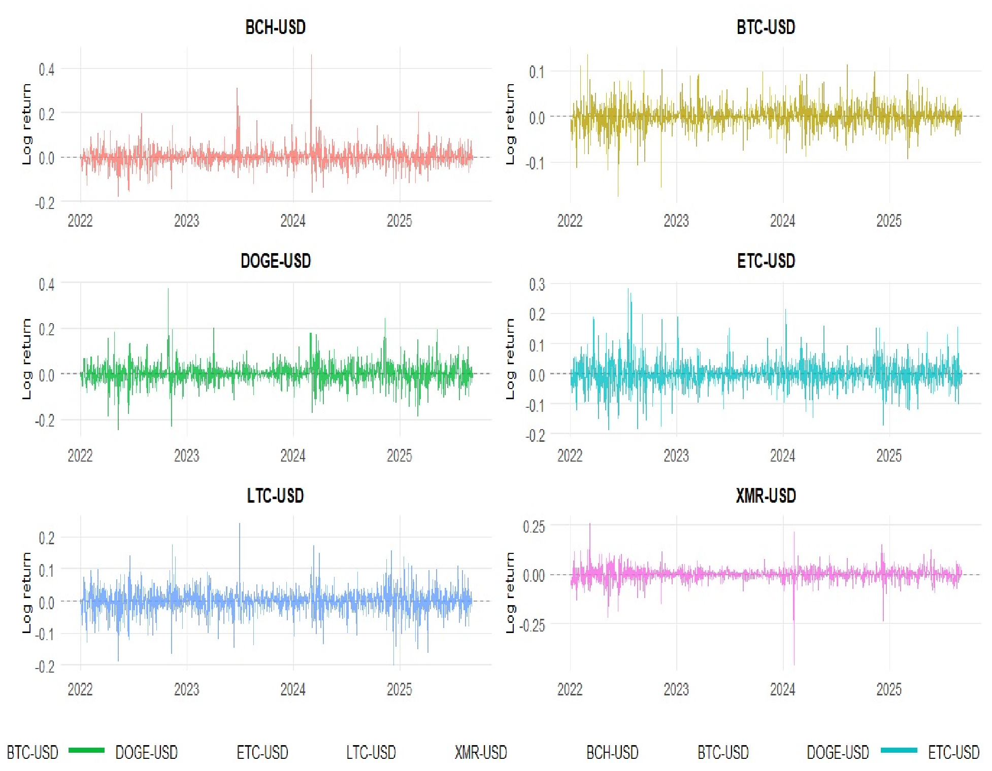
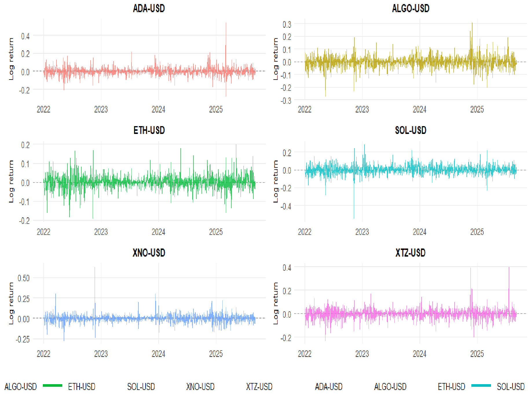
Figure 1 and Figure 2 show the daily log returns of the 12 cryptocurrencies over the full sample period. The return series fluctuate around zero and display high volatility, with the amplitude of the movements increasing markedly during several episodes between 2022 and 2025. Volatility is not constant over time and alternates between calm periods and sudden spikes. This pattern is consistent with conditional heteroskedasticity and supports the use of a tail-risk measure rather than a variance-based one. The environmental classification used in the portfolio analysis is period-specific, as defined in Section 3.1.

Table 2. Descriptive statistics of the daily log returns.

Asset	Mean	Median	Max.	Min.	Std. Dev.	Skew.	Kurt.	Jarque-Bera
BTC	0.0006	−0.0002	0.1358	−0.1741	0.0275	−0.151	7.45	1113.4
BCH	0.0002	−0.0001	0.4601	−0.1766	0.0436	1.301	15.89	9680.2
LTC	−0.0002	0.0009	0.2437	−0.1985	0.0400	−0.141	6.91	860.1
XMR	0.0000	0.0023	0.2593	−0.4544	0.0370	−1.507	25.35	28,476.1
ETC	−0.0004	−0.0011	0.2815	−0.1875	0.0451	0.549	7.89	1407.7
DOGE	0.0002	−0.0003	0.3712	−0.2488	0.0484	0.403	8.70	1855.9
ETH	0.0001	0.0003	0.1972	−0.1918	0.0367	−0.040	7.21	993.9
ADA	−0.0004	−0.0009	0.5384	−0.2781	0.0455	1.149	20.21	16,886.2
SOL	0.0001	−0.0010	0.2821	−0.5496	0.0523	−0.720	14.18	7114.2
ALGO	−0.0015	0.0012	0.3078	−0.2731	0.0485	−0.015	7.10	941.8
XTZ	−0.0014	0.0011	0.3970	−0.2312	0.0448	0.671	13.64	6440.1
XNO	−0.0011	−0.0003	0.6279	−0.2731	0.0488	1.627	27.27	33,577.9

Note: Each series has 1344 daily observations. The Jarque-Bera test rejects the null hypothesis of normality for all series ($p<0.001$).

reports the descriptive statistics of the return series. Mean daily returns are close to zero for all assets. Among the twelve cryptocurrencies, BTC has the highest mean return (0.0006) and the lowest standard deviation (0.0275). ETH also displays comparatively low dispersion, with a standard deviation of 0.0367 and a small positive mean return. The standard deviations of the remaining assets lie between 0.0370 and 0.0523. The maximum and minimum values also show the presence of extreme movements, including single-day changes exceeding 50% in absolute value for ADA, SOL, and XNO.

All series depart from normality. Kurtosis exceeds the Gaussian value of three for every asset and reaches particularly high levels for XMR (25.35), XNO (27.27), and ADA (20.21), indicating leptokurtic and heavy-tailed return distributions. The skewness coefficients also indicate asymmetry in several return series. The Jarque–Bera test rejects the null hypothesis of normality for all twelve series. These features confirm the non-normal and heavy-tailed behavior of cryptocurrency returns and support the use of CVaR as the risk measure in the portfolio optimization.

Table 3. Stationarity and autocorrelation tests of the daily log returns.

Asset	ADF	KPSS	LB	LB p-Value	LB Decision
BTC	−37.71	0.4113	24.53	0.2202	No autocorrelation
BCH	−38.19	0.2866	26.69	0.1441	No autocorrelation
LTC	−37.58	0.1836	28.86	0.0906	No autocorrelation
XMR	−41.44	0.1508	32.89	0.0347	Autocorrelation
ETC	−36.97	0.0377	46.65	0.0007	Autocorrelation
DOGE	−37.03	0.1391	32.13	0.0419	Autocorrelation
ETH	−37.61	0.2451	20.73	0.4131	No autocorrelation
ADA	−38.33	0.2832	32.25	0.0407	Autocorrelation
SOL	−36.99	0.4638	17.89	0.5945	No autocorrelation
ALGO	−36.06	0.4059	23.70	0.2558	No autocorrelation
XTZ	−39.53	0.1787	28.37	0.1010	No autocorrelation
XNO	−36.92	0.2267	37.15	0.0112	Autocorrelation

Note: The ADF null hypothesis of a unit root is rejected for all series at the 1% level ($p<0.001$). The KPSS null hypothesis of stationarity is not rejected for any series (5% critical value = $0.463$). The Ljung–Box (LB) test is evaluated at the 5% level.

summarizes the results of the stationarity and autocorrelation tests. The ADF test rejects the null hypothesis of a unit root for every series at the 1% level, indicating that the log returns are stationary. The KPSS test, whose null hypothesis is stationarity, does not reject stationarity for any series. The results of both tests confirm that the return series are stationary and can be used directly in optimization.

The Ljung–Box test provides a heterogeneous picture. For BTC, BCH, LTC, ETH, SOL, ALGO, and XTZ, the null hypothesis of no autocorrelation is not rejected at the 5% level. By contrast, XMR, ETC, DOGE, ADA, and XNO show statistically significant autocorrelation, indicating some temporal dependence in their returns. These results characterize the individual return series and do not alter the cross-sectional portfolio optimization that follows.

4.2. Mixed Universe

To compare the portfolio allocations obtained using the three algorithms, this section first considers the Mixed universe. This universe contains all 12 cryptocurrencies in both periods and allows the algorithms to select assets from the full investment set.

Table 4. Mean-CVaR portfolio results for the Mixed universe before and after the Ethereum Merge.

	NSGA-II	SPEA2	PSO
Panel A: Pre-Merge period
BTC	0.3727	0.7441	0.0000
LTC	0.0745	0.0006	0.0032
DOGE	0.0022	0.0008	0.0014
XMR	0.1652	0.0251	0.0000
BCH	0.0034	0.0000	0.0000
ETC	0.2665	0.2192	0.9910
ETH	0.0931	0.0021	0.0000
ALGO	0.0011	0.0013	0.0006
ADA	0.0141	0.0015	0.0000
XTZ	0.0040	0.0035	0.0013
SOL	0.0029	0.0010	0.0000
XNO	0.0003	0.0007	0.0025
CVaR	0.1074	0.0999	0.1305
Return	−0.002154	−0.002491	0.000425
Panel B: Post-Merge period
BTC	0.6743	0.8722	0.3524
LTC	0.0006	0.0000	0.0004
DOGE	0.0069	0.0001	0.0019
XMR	0.0212	0.0000	0.0010
BCH	0.1687	0.0006	0.2571
ETC	0.0020	0.0000	0.0000
ETH	0.0082	0.0002	0.0000
ALGO	0.0013	0.0000	0.0000
ADA	0.0055	0.0001	0.0000
XTZ	0.0008	0.0000	0.0002
SOL	0.1085	0.1265	0.3870
XNO	0.0020	0.0000	0.0000
CVaR	0.0611	0.0584	0.0752
Return	0.001527	0.001591	0.001584

Note: Panel A covers the Pre-Merge period from January 2022 to 14 September 2022. Panel B covers the Post-Merge period from 16 September 2022 to September 2025. All portfolios are optimized at the 95% CVaR confidence level. Weights below 0.0001 are reported as 0.0000.

reports the portfolio weights, expected returns, and CVaR values obtained with NSGA-II, SPEA2, and PSO at the 95% confidence level.

During the Pre-Merge period, NSGA-II and SPEA2 obtain CVaR values of 0.1074 and 0.0999, respectively, with negative expected returns. Their portfolios are mainly concentrated in BTC and ETC. NSGA-II also retains larger positions in XMR, ETH, and LTC. PSO achieves a positive expected return of 0.000425 with a CVaR of 0.1305 and allocates approximately 99% of the portfolio to ETC. During the Pre-Merge period, the Mixed portfolios are therefore largely concentrated in energy-intensive assets across the three optimization methods.

In the Post-Merge period, the three algorithms produce positive expected returns between 0.001527 and 0.001591, with CVaR values between 0.0584 and 0.0752. BTC receives the largest weight under NSGA-II and SPEA2, at 67.4% and 87.2%, respectively, while PSO allocates most of the portfolio to SOL, BTC, and BCH. Despite these differences in composition, the three methods generate very similar expected returns. In addition, Post-Merge CVaR values are lower than the corresponding Pre-Merge values for all three algorithms.

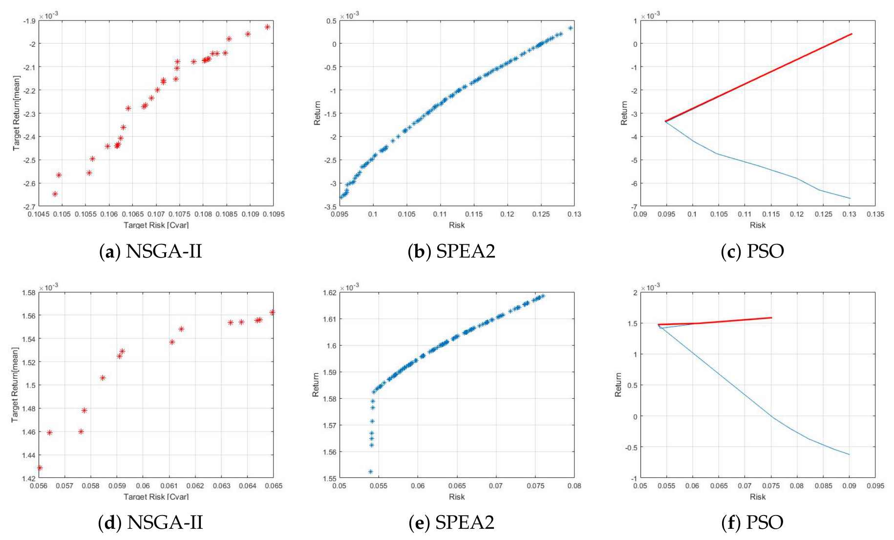
Figure 3 illustrates the Mean-CVaR efficient frontiers. The Post-Merge portfolios exhibit positive expected returns and lower CVaR values than the corresponding Pre-Merge portfolios under NSGA-II, SPEA2, and PSO. The figure also shows the expected risk–return trade-off, with higher expected returns associated with higher CVaR values along the frontier.

4.3. Dirty Universe

To assess the consistency of the results observed in the Mixed universe when the investment universe is restricted to energy-intensive cryptocurrencies, this section examines the Dirty universe. Its composition differs across the two periods because ETH is included before the Merge and excluded after the transition to Proof-of-Stake.

Table 5. Mean-CVaR portfolio results for the Dirty universe before and after the Ethereum Merge.

	NSGA-II	SPEA2	PSO
Panel A: Pre-Merge period
BTC	0.6899	0.9415	0.0000
LTC	0.0001	0.0015	0.0000
DOGE	0.0004	0.0000	0.0000
XMR	0.0023	0.0005	0.0000
BCH	0.0000	0.0000	0.0000
ETC	0.3069	0.0550	1.0000
ETH	0.0003	0.0013	0.0000
CVaR	0.1020	0.0957	0.1307
Return	−0.002173	−0.003137	0.000470
Panel B: Post-Merge period
BTC	0.9952	0.9967	1.0000
LTC	0.0000	0.0000	0.0000
DOGE	0.0000	0.0000	0.0000
XMR	0.0048	0.0032	0.0000
BCH	0.0000	0.0000	0.0000
ETC	0.0000	0.0000	0.0000
CVaR	0.0542	0.0542	0.0543
Return	0.001578	0.001579	0.001583

Note: ETH belongs to the Dirty universe during the Pre-Merge period and is excluded from this universe after its transition to Proof-of-Stake. All portfolios are optimized at the 95% CVaR confidence level. Weights below 0.0001 are reported as 0.0000.

reports the portfolio weights, expected returns, and CVaR values obtained using NSGA-II, SPEA2, and PSO at the 95% confidence level.

During the Pre-Merge period, BTC and ETC account for most of the Dirty portfolio under the three optimization methods. NSGA-II allocates 69.0% to BTC and 30.7% to ETC, whereas SPEA2 assigns 94.2% to BTC and 5.5% to ETC. PSO concentrates the portfolio in ETC. The corresponding CVaR values lie between 0.0957 and 0.1307. ETH receives only a small allocation under NSGA-II and SPEA2 and no allocation under PSO. These results show that, although ETH is included in the Dirty universe during the Pre-Merge period, the selected portfolios are dominated by BTC and ETC.

The Post-Merge results indicate a more consistent allocation across the three algorithms. Specifically, NSGA-II allocates 99.5% of the portfolio to BTC, SPEA2 allocates 99.7%, and PSO allocates the entire portfolio to BTC. The expected returns are also similar, ranging from 0.001578 to 0.001583, while the CVaR values lie between 0.0542 and 0.0543. Consequently, the three algorithms identify nearly identical risk–return outcomes for the Post-Merge Dirty universe.

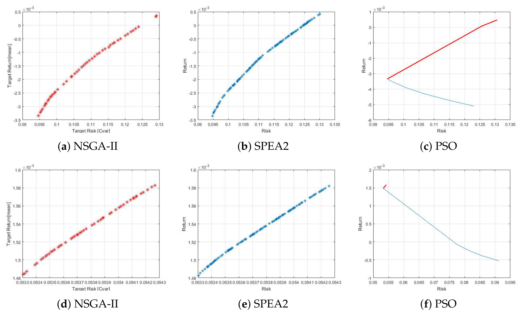
Figure 4 illustrates the corresponding efficient frontiers. Compared with the Pre-Merge results, the selected Post-Merge portfolios exhibit positive expected returns and lower CVaR values under all three algorithms. Notably, the Post-Merge Dirty universe produces the closest agreement among NSGA-II, SPEA2, and PSO in terms of both portfolio composition and the resulting risk–return values.

The next section examines the Green universe, where ETH enters the investment universe after its transition to Proof-of-Stake.

4.4. Green Universe

To complete the comparison across the three investment universes, this section considers the Green universe. Its composition changes after the Merge. Before the Merge, the universe contains ADA, SOL, ALGO, XTZ, and XNO. After ETH transitions to Proof-of-Stake, it enters the Green universe.

Table 6. Mean-CVaR portfolio results for the Green universe before and after the Ethereum Merge.

	NSGA-II	SPEA2	PSO
Panel A: Pre-Merge period
ALGO	0.3188	0.3557	0.3714
ADA	0.4023	0.4020	0.4066
XTZ	0.1873	0.1383	0.1264
SOL	0.0000	0.0000	0.0000
XNO	0.0916	0.1040	0.0956
CVaR	0.1225	0.1224	0.1224
Return	−0.005124	−0.005235	−0.005265
Panel B: Post-Merge period
ETH	0.6332	0.9341	0.0000
ALGO	0.0000	0.0003	0.0000
ADA	0.0004	0.0021	0.0000
XTZ	0.0000	0.0001	0.0000
SOL	0.3659	0.0000	1.0000
XNO	0.0004	0.0633	0.0000
CVaR	0.0821	0.0764	0.1064
Return	0.001225	0.000918	0.001656

Note: The Pre-Merge Green universe contains ADA, SOL, ALGO, XTZ, and XNO. ETH enters the Green universe after its transition to Proof-of-Stake. All portfolios are optimized at the 95% CVaR confidence level. Weights below 0.0001 are reported as 0.0000.

reports the portfolio weights, expected returns, and CVaR values obtained using NSGA-II, SPEA2, and PSO at the 95% confidence level.

During the Pre-Merge period, the three algorithms produce closely comparable results for the Green universe. CVaR remains around 0.1224, while expected returns range from −0.005265 to −0.005124. The portfolio composition is also similar across the three methods. ADA receives approximately 40% of the portfolio, followed by ALGO, XTZ, and XNO. SOL does not receive any material weight. Thus, NSGA-II, SPEA2, and PSO identify a similar Green portfolio when ETH is not included in the investment universe.

The portfolio structure changes in the Post-Merge period after ETH enters the Green universe. NSGA-II allocates 63.3% to ETH and 36.6% to SOL, while SPEA2 assigns 93.4% to ETH and 6.3% to XNO. PSO allocates the entire portfolio to SOL. All three portfolios generate positive expected returns between 0.000918 and 0.001656, with CVaR values between 0.0764 and 0.1064. Relative to the Pre-Merge period, the selected Post-Merge portfolios exhibit lower CVaR values and higher expected returns under all three optimization methods.

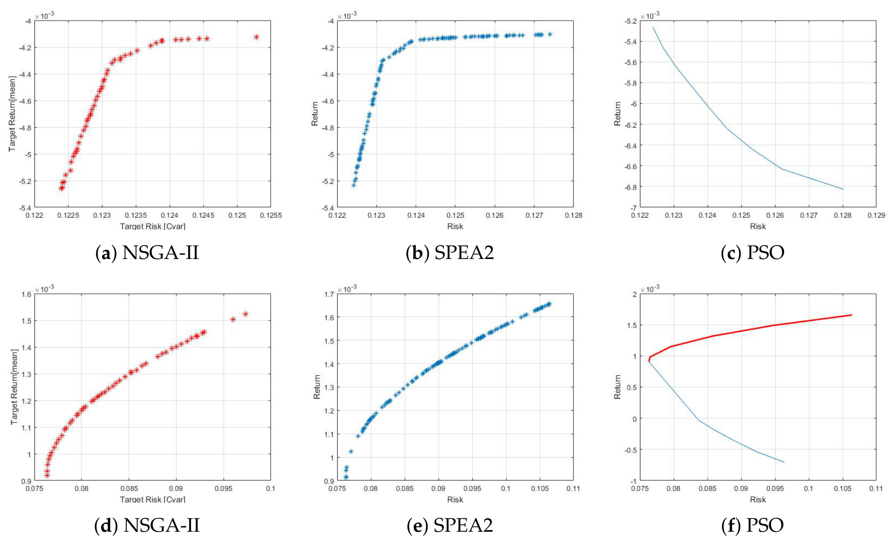
Figure 5 illustrates the corresponding efficient frontiers. The Post-Merge results also allow a comparison across the three investment universes. Under NSGA-II, SPEA2, and PSO, the Green universe exhibits higher CVaR values than the corresponding Dirty and Mixed portfolios. This ordering is consistent across the three optimization methods and constitutes the main empirical result examined in the robustness analysis that follows.

4.5. Robustness and Validation of the Three Optimization Algorithms

To assess the robustness of the results obtained with NSGA-II, SPEA2, and PSO, this section considers two distinct sensitivity exercises. First, Panel A examines sensitivity to the tail-risk specification by increasing the CVaR confidence level from 95% to 99%. Second, Panels B and C examine portfolio concentration by imposing maximum individual asset weights. For these concentration tests, the CVaR confidence level is retained at 95%, as in the main analysis, so that the effect of the weight restriction can be assessed while holding the risk specification unchanged.

Table 7. Mean-CVaR results under alternative tail-risk and portfolio concentration specifications.

Universe	Algorithm	Expected Return	CVaR
Panel A: CVaR confidence level of 99%
Green	NSGA-II	0.001496	0.168400
Green	SPEA2	0.000942	0.121388
Green	PSO	0.001656	0.187222
Dirty	NSGA-II	0.001569	0.084429
Dirty	SPEA2	0.001440	0.082186
Dirty	PSO	0.001583	0.084735
Mixed	NSGA-II	0.001481	0.092276
Mixed	SPEA2	0.001522	0.083351
Mixed	PSO	0.001595	0.122021
Panel B: Maximum asset weight of 33.33% at the 95% CVaR confidence level
Green	NSGA-II	0.001050	0.084702
Green	SPEA2	0.001049	0.084663
Green	PSO	0.001050	0.084702
Dirty	NSGA-II	0.001234	0.063587
Dirty	SPEA2	0.001234	0.063560
Dirty	PSO	0.001419	0.076153
Mixed	NSGA-II	0.001537	0.072536
Mixed	SPEA2	0.001552	0.073229
Mixed	PSO	0.001576	0.074373
Panel C: Maximum asset weight of 10% at the 95% CVaR confidence level
Mixed	NSGA-II	0.000842	0.078239
Mixed	SPEA2	0.000841	0.078225
Mixed	PSO	0.000842	0.078239

Note: All results are obtained over the Post-Merge period. Panel A examines sensitivity to the CVaR confidence level using 99%. Panels B and C examine portfolio concentration and retain the 95% CVaR confidence level used in the main analysis. The 10% maximum weight is feasible only for the Mixed universe under the full-investment constraint.

reports the results.

Increasing the CVaR confidence level from 95% to 99% raises the estimated tail risk across all three universes. However, the main universe-level ranking remains unchanged. The Green universe has the highest CVaR under NSGA-II, SPEA2, and PSO. Its CVaR values lie between 0.1214 and 0.1872, compared with values between 0.0822 and 0.0847 for the Dirty universe and between 0.0834 and 0.1220 for the Mixed universe. Thus, the three algorithms preserve the same tail-risk ranking when the analysis focuses on more extreme losses.

The results remain consistent when portfolio concentration is restricted. Under the 33.33% maximum weight, the Green universe has the highest CVaR and the lowest expected return under all three algorithms. Moreover, the Green portfolios produce almost identical outcomes across the three methods, with an expected return close to 0.00105 and a CVaR close to 0.0847. The corresponding CVaR values remain lower for the Dirty and Mixed universes. Therefore, the main comparison obtained with NSGA-II, SPEA2, and PSO does not depend on allowing a single cryptocurrency to dominate the portfolio.

A more restrictive 10% weight limit can be applied to the Mixed universe because it contains 12 assets. Under this restriction, the three algorithms produce nearly identical risk–return outcomes. Expected returns are approximately 0.000842, while CVaR values are approximately 0.07823 under NSGA-II, SPEA2, and PSO. The close agreement across the three methods indicates greater consistency in portfolio outcomes when individual asset weights are subject to more restrictive limits.

The two sensitivity exercises further support the consistency of the main results across the three optimization algorithms. In particular, the Green universe continues to exhibit higher CVaR than the Dirty and Mixed universes under the alternative tail-risk and portfolio-concentration specifications, while the constrained portfolios produce more similar risk–return outcomes across NSGA-II, SPEA2, and PSO.

To further assess the performance of the three optimization algorithms, this section compares their minimum-CVaR solutions with an exact mathematical programming benchmark. Comparing evolutionary portfolio optimization methods with exact counterparts provides a direct way to assess how closely heuristic solutions approach the mathematical optimum (Ferreira and Cardoso 2021). Accordingly, the exact minimum-CVaR portfolio is obtained using MATLAB R2025a over the Post-Merge period at the 95% confidence level for the Green, Dirty, and Mixed universes.

$${\Delta }_A=CVa{R}_{\min }^A-CVa{R}_{\min }^{LP},$$

where A denotes NSGA-II, SPEA2, or PSO, and $CVa{R}_{\min }^{LP}$ is the exact minimum obtained with MATLAB linprog. A smaller value of ${\Delta }_A$ indicates a closer approximation to the exact minimum-CVaR solution.

Table 8. Differences between the evolutionary solutions and the exact minimum-CVaR benchmark.

Universe	ΔNSGA-II	ΔSPEA2	ΔPSO
Green	0.00577	0.00002	0.03004
Dirty	0.00091	0.00093	0.00096
Mixed	0.00784	0.00506	0.02188

Note: Each difference is calculated as the minimum CVaR obtained by the corresponding evolutionary algorithm minus the exact minimum CVaR obtained with MATLAB linprog. All calculations use the Post-Merge period and a 95% CVaR confidence level.

reports the results.

Table 8 shows that the SPEA2 solutions differ from their corresponding exact minimum-CVaR benchmarks by 0.00002, 0.00093, and 0.00506 for the Green, Dirty, and Mixed universes, respectively. For the Dirty universe, all three algorithms are particularly close to the exact solution, with differences between 0.00091 and 0.00096. This result is consistent with the similar Dirty portfolio outcomes reported in Section 4.3.

The exact benchmark also preserves the main universe-level tail-risk ranking. The minimum CVaR is 0.076334 for the Green universe and approximately 0.053304 for both the Dirty and Mixed universes. Thus, the exact optimization confirms the higher minimum CVaR of the Green universe observed with the three population-based algorithms. The benchmark therefore provides additional support for the main cross-universe comparison.

Finally, this section examines the temporal robustness of the results obtained with NSGA-II, SPEA2, and PSO. The Post-Merge sample is divided into two consecutive subperiods: 16 September 2022 to 31 March 2024 ($S_1$) and 1 April 2024 to 30 September 2025 ($S_2$). The Mean-CVaR optimization is repeated for the Green, Dirty, and Mixed universes using the same 95% confidence level as in the main analysis.

Table 9. Mean-CVaR results across the Post-Merge subperiods.

Universe	Algorithm	${\mathit{S}}_1$		${\mathit{S}}_2$
		Return	CVaR	Return	CVaR
Green	NSGA-II	0.001909	0.071598	0.000323	0.085094
Green	SPEA2	0.003169	0.115716	0.000430	0.104747
Green	PSO	0.003223	0.117758	0.000434	0.105771
Dirty	NSGA-II	0.002070	0.054794	0.001255	0.062895
Dirty	SPEA2	0.002216	0.055586	0.001383	0.072796
Dirty	PSO	0.003114	0.079034	0.001397	0.074019
Mixed	NSGA-II	0.002161	0.061301	0.001026	0.055153
Mixed	SPEA2	0.002861	0.068529	0.001019	0.052425
Mixed	PSO	0.003148	0.087756	0.001147	0.057795

Note: $S_1$ covers 16 September 2022 to 31 March 2024 and $S_2$ covers 1 April 2024 to 30 September 2025. All portfolios are optimized at the 95% CVaR confidence level.

reports the selected portfolio outcomes.

The subperiod analysis confirms the main risk comparison obtained over the full Post-Merge sample. In $S_1$, the Green universe exhibits the highest CVaR under each of the three algorithms. Its CVaR is 0.071598 under NSGA-II, 0.115716 under SPEA2, and 0.117758 under PSO. The corresponding values are lower for both the Dirty and Mixed universes.

The same ordering is observed in $S_2$. The Green universe has a CVaR of 0.085094 under NSGA-II, 0.104747 under SPEA2, and 0.105771 under PSO. These values remain above those obtained for the Dirty and Mixed universes under the corresponding algorithms. Thus, the higher CVaR of the Green universe is observed in both parts of the Post-Merge sample.

Portfolio compositions differ across the two subperiods as the relative risk–return characteristics of the available assets change. However, these differences do not alter the main comparison across the investment universes. NSGA-II, SPEA2, and PSO all identify the Green universe as having the highest CVaR in both subperiods. The subperiod analysis therefore provides additional evidence that the main risk comparison remains consistent across different parts of the Post-Merge period.

As an additional sensitivity check, this analysis examines whether the effect of asset exclusion depends on the cryptocurrency removed from the investment universe. Starting from the Post-Merge Mixed universe at the 95% CVaR confidence level, the optimization is repeated after excluding BTC and, separately, after excluding ETH.

Table 10. Asset-exclusion sensitivity for the Post-Merge Mixed universe.

Specification	Algorithm	Return	CVaR
Without BTC	NSGA-II	0.001007	0.069409
	SPEA2	0.001476	0.082208
	PSO	0.001575	0.088979
Without ETH	NSGA-II	0.001491	0.063662
	SPEA2	0.001572	0.054175
	PSO	0.001569	0.069095

Note: The analysis uses the Post-Merge Mixed universe and a 95% CVaR confidence level. BTC and ETH are excluded separately from the investment universe.

reports the corresponding results.

The exclusion of BTC increases CVaR relative to the unrestricted Mixed universe under all three algorithms. The effect differs when ETH is excluded. In this case, CVaR changes only modestly under NSGA-II and is lower under SPEA2 and PSO than in the corresponding unrestricted portfolios. The effect of removing an asset therefore depends on the risk–return characteristics of the cryptocurrency excluded from the investment universe.

This result also helps to explain the difference between the Green and Dirty portfolios. The effect of restricting the investment universe depends on which cryptocurrency is excluded. In the present sample, excluding BTC leads to a larger increase in CVaR than excluding ETH, and this result is consistent across NSGA-II, SPEA2, and PSO.

5. Discussion

The results of this study show that environmental restrictions affect cryptocurrency portfolio risk by changing the assets available for investment. In the Post-Merge period, the Green universe exhibits a higher CVaR than the Dirty and Mixed universes under NSGA-II, SPEA2, and PSO. This finding remains consistent across the robustness analyses and is also confirmed by the exact optimization benchmark.

This result reflects differences in the composition of the investment universes, particularly the availability of BTC in the Dirty and Mixed universes and its exclusion from the Green universe. BTC receives a large weight in the Dirty and Mixed portfolios, while it is not available to the Green portfolio. The asset-exclusion analysis provides further support for this interpretation. Removing BTC from the Mixed universe increases CVaR under all three algorithms, whereas removing ETH does not produce the same systematic increase. Therefore, the effect of an environmental restriction depends on the asset removed from the investment universe. This finding also indicates that the higher CVaR of the Green universe should not be interpreted as evidence that Green cryptocurrencies are inherently riskier.

These findings complement previous research on Green cryptocurrency diversification. Pham et al. (2022), Naeem et al. (2023), and Ali et al. (2024) provide evidence on dependence, spillovers, and diversification between Green cryptocurrencies and other assets. The present findings are consistent with these studies. They show that diversification potential does not directly determine optimal portfolio weights. The present study extends this literature by examining how environmentally classified cryptocurrencies compete for capital under a common Mean-CVaR objective.

The important role of BTC is also consistent with previous cryptocurrency allocation studies. Ma et al. (2020) and Som and Kayal (2022) report important portfolio effects from the inclusion of BTC, while Bakry et al. (2021) show that its portfolio allocation is affected by investment constraints. In the present study, BTC receives large weights in the baseline Dirty and Mixed portfolios. However, the main risk comparison remains when individual portfolio weights are restricted. This result provides further evidence that the higher CVaR of the Green universe is not limited to highly concentrated portfolios.

Another important finding is the consistency of the results across the three optimization methods. NSGA-II, SPEA2, and PSO identify the Green universe as having the highest CVaR in the Post-Merge analysis. The same ordering is observed at the 99% confidence level and in both Post-Merge subperiods. The exact linear-programming benchmark provides additional validation. Comparing evolutionary portfolio methods with exact mathematical programming solutions provides a useful benchmark for evaluating heuristic solutions (Ferreira and Cardoso 2021). In the present study, the exact benchmark preserves the same risk ranking across the three investment universes. This finding supports the view that the main result reflects the composition of the investment universe rather than the behavior of a particular optimization method.

The findings also have practical implications for ESG-oriented investors. Environmental screening changes the investment universe and may exclude an asset that plays an important role in the optimal portfolio. The results therefore suggest that the financial effect of an environmental restriction depends not only on the environmental classification of an asset but also on its role in the portfolio risk-return trade-off. In addition, the results under portfolio weight limits show that the higher CVaR of the Green universe remains when concentration is restricted. More generally, the findings distinguish diversification evidence from direct portfolio allocation. Dependence measures describe how assets move together, whereas portfolio optimization determines how capital is allocated under a specific objective. The present analysis therefore focuses on how environmental classification affects portfolio weights and CVaR under a common optimization framework.

The findings are conditional on the cryptocurrencies included in the investment universe and the study period. Therefore, they should be interpreted as evidence for the investment universes considered in this study rather than as a general ranking of all Green and energy-intensive cryptocurrencies.

6. Conclusions

This study examines the effect of environmental restrictions on cryptocurrency portfolio allocation under a Mean-CVaR framework. Green, Dirty, and Mixed investment universes are optimized using NSGA-II, SPEA2, and PSO, with ETH classified according to its consensus mechanism before and after the Merge.

The results show that the composition of the investment universe has an important effect on portfolio CVaR. In the Post-Merge period, the Green universe exhibits a higher CVaR than the Dirty and Mixed universes under all three algorithms. This finding remains consistent across the additional analyses, indicating that the main comparison is not specific to a particular optimization method or specification.

One important contribution of this study is that it extends the Green cryptocurrency literature from dependence and diversification analysis to direct portfolio allocation. The findings show that environmental screening affects portfolio outcomes through the assets that remain available for investment. Therefore, the financial effect of such a restriction depends on the composition of the investment universe.

References

1. Abdallah, Ameni Ben Hadj, Rihab Bedoui, and Heni Boubaker. 2025. Metaheuristics for Portfolio Optimization: Application of NSGAII, SPEA2, and PSO Algorithms. Risks 13: 227. [Google Scholar] [CrossRef] [Scilit]
2. Acerbi, Carlo, and Dirk Tasche. 2002. On the Coherence of Expected Shortfall. Journal of Banking & Finance 26: 1487–503. [Google Scholar] [CrossRef] [Scilit]
3. Ali, Shujaat, Muhammad Naveed, Imran Yousaf, and Muhammad Saeed Khattak. 2024. From Cryptos to Consciousness: Dynamics of Return and Volatility Spillover between Green Cryptocurrencies and G7 Markets. Finance Research Letters 60: 104899. [Google Scholar] [CrossRef] [Scilit]
4. Artzner, Philippe, Freddy Delbaen, Jean-Marc Eber, and David Heath. 1997. Thinking Coherently. Risk 10: 68–71. [Google Scholar]
5. Artzner, Philippe, Freddy Delbaen, Jean-Marc Eber, and David Heath. 1999. Coherent Measures of Risk. Mathematical Finance 9: 203–28. [Google Scholar] [CrossRef] [Scilit]
6. Bakry, Walid, Audil Rashid, Somar Al-Mohamad, and Nasser El-Kanj. 2021. Bitcoin and Portfolio Diversification: A Portfolio Optimization Approach. Journal of Risk and Financial Management 14: 282. [Google Scholar] [CrossRef] [Scilit]
7. Bedoui, Rihab, Ramzi Benkraiem, Khaled Guesmi, and Islem Kedidi. 2023. Portfolio Optimization through Hybrid Deep Learning and Genetic Algorithms Vine Copula-GARCH-EVT-CVaR Model. Technological Forecasting and Social Change 197: 122887. [Google Scholar] [CrossRef] [Scilit]
8. Boubaker, Heni, and Nadia Sghaier. 2013. Portfolio Optimization in the Presence of Dependent Financial Returns with Long Memory: A Copula-Based Approach. Journal of Banking & Finance 37: 361–77. [Google Scholar] [CrossRef] [Scilit]
9. Deb, Kalyanmoy, Amrit Pratap, Sameer Agarwal, and T. Meyarivan. 2002. A Fast and Elitist Multiobjective Genetic Algorithm: NSGA-II. IEEE Transactions on Evolutionary Computation 6: 182–97. [Google Scholar] [CrossRef] [Scilit]
10. Duan, Kun, Yanqi Zhao, Andrew Urquhart, and Yingying Huang. 2023. Do Clean and Dirty Cryptocurrencies Connect with Financial Assets Differently? The Role of Economic Policy Uncertainty. Energy Economics 127: 107079. [Google Scholar] [CrossRef] [Scilit]
11. Ferreira, Fernando G. D. C., and Rodrigo T. N. Cardoso. 2021. Mean-CVaR Portfolio Optimization Approaches with Variable Cardinality Constraint and Rebalancing Process. Archives of Computational Methods in Engineering 28: 3703–20. [Google Scholar] [CrossRef] [Scilit]
12. Ghanbari, Hamid, Ehsan Mohammadi, Amir Masoud Larni-Fooeik, R. Ramesh Kumar, Peter Jan Stauvermann, and Mohammad Shabani. 2024. Cryptocurrency Portfolio Allocation under Credibilistic CVaR Criterion and Practical Constraints. Risks 12: 163. [Google Scholar] [CrossRef] [Scilit]
13. Guarino, Alfonso, Domenico Santoro, Luca Grilli, Rocco Zaccagnino, and Mario Balbi. 2024. EvoFolio: A Portfolio Optimization Method Based on Multi-Objective Evolutionary Algorithms. Neural Computing and Applications 36: 7221–43. [Google Scholar] [CrossRef] [Scilit]
14. Hotta, Luiz K., Eduardo C. Lucas, and Helder P. Palaro. 2008. Estimation of VaR Using Copula and Extreme Value Theory. Multinational Finance Journal 12: 205–18. Available online: https://ideas.repec.org/a/mfj/journl/v12y2008i3-4p205-218.html (accessed on 1 August 2026). [CrossRef] [Scilit]
15. Kapengut, Elie, and Bruce Mizrach. 2023. An Event Study of the Ethereum Transition to Proof-of-Stake. Commodities 2: 96–110. [Google Scholar] [CrossRef] [Scilit]
16. Kaucic, Massimiliano, Mojtaba Moradi, and Mohmmad Mirzazadeh. 2019. Portfolio Optimization by Improved NSGA-II and SPEA 2 Based on Different Risk Measures. Financial Innovation 5: 26. [Google Scholar] [CrossRef] [Scilit]
17. Khaki, Audil Rashid, Somar Al-Mohamad, Ammar Jreisat, Fadia Al-Hajj, and Mustafa Raza Rabbani. 2022. Portfolio Diversification of MENA Markets with Cryptocurrencies: Mean-Variance vs Higher-Order Moments Approach. Scientific African 17: e01303. [Google Scholar] [CrossRef] [Scilit]
18. Krokhmal, Pavlo, Jonas Palmquist, and Stanislav Uryasev. 2002. Portfolio Optimization with Conditional Value-at-Risk Objective and Constraints. The Journal of Risk 4: 43–68. [Google Scholar] [CrossRef] [Scilit]
19. Liu, Yue, Huaping Sun, Bo Meng, Shunlin Jin, and Bin Chen. 2023. How to purchase carbon emission right optimally for energy-consuming enterprises? Analysis based on optimal stopping model. Energy Economics 124: 106758. [Google Scholar] [CrossRef] [Scilit]
20. Liu, Yue, Lixin Tian, Boyan Zou, Peiyuan Zhao, and Chenyang Gan. 2026. Multi-source carbon emission monitoring and certification for carbon-neutral industrial parks. Journal of Cleaner Production 570: 148612. [Google Scholar] [CrossRef] [Scilit]
21. Ma, Ying, Farid Ahmad, Meng Liu, and Zhen Wang. 2020. Portfolio Optimization in the Era of Digital Financialization Using Cryptocurrencies. Technological Forecasting and Social Change 161: 120265. [Google Scholar] [CrossRef] [Scilit] [PubMed]
22. Markowitz, Harry. 1952. Portfolio Selection. The Journal of Finance 7: 77–91. [Google Scholar] [CrossRef] [Scilit]
23. Mba, Jules Clément, and Magdaline Mbong Mai. 2022. A Particle Swarm Optimization Copula-Based Approach with Application to Cryptocurrency Portfolio Optimisation. Journal of Risk and Financial Management 15: 285. [Google Scholar] [CrossRef] [Scilit]
24. Naeem, Muhammad Abubakr, Thi Thu Ha Nguyen, Sitara Karim, and Brian M. Lucey. 2023. Extreme Downside Risk Transmission between Green Cryptocurrencies and Energy Markets: The Diversification Benefits. Finance Research Letters 58: 104263. [Google Scholar] [CrossRef] [Scilit]
25. Pham, Linh, Sitara Karim, Muhammad Abubakr Naeem, and Chao Long. 2022. A Tale of Two Tails among Carbon Prices, Green and Non-Green Cryptocurrencies. International Review of Financial Analysis 82: 102139. [Google Scholar] [CrossRef] [Scilit]
26. Rockafellar, R. Tyrrell, and Stanislav Uryasev. 2000. Optimization of Conditional Value-at-Risk. The Journal of Risk 2: 21–41. [Google Scholar] [CrossRef] [Scilit]
27. Rockafellar, R. Tyrrell, and Stanislav Uryasev. 2002. Conditional Value-at-Risk for General Loss Distributions. Journal of Banking & Finance 26: 1443–71. [Google Scholar] [CrossRef] [Scilit]
28. Sahamkhadam, Maziar, Andreas Stephan, and Ralf Östermark. 2018. Portfolio Optimization Based on GARCH-EVT-Copula Forecasting Models. International Journal of Forecasting 34: 497–506. [Google Scholar] [CrossRef] [Scilit]
29. Som, Ankit, and Parthajit Kayal. 2022. A Multicountry Comparison of Cryptocurrency vs Gold: Portfolio Optimization through Generalized Simulated Annealing. Blockchain: Research and Applications 3: 100075. [Google Scholar] [CrossRef] [Scilit]
30. Umar, Zaghum, Onur Polat, Sun-Yong Choi, and Tamara Teplova. 2022. The Impact of the Russia-Ukraine Conflict on the Connectedness of Financial Markets. Finance Research Letters 48: 102976. [Google Scholar] [CrossRef] [Scilit]
31. Xu, Fasheng, Wei Chen, and Ling Yang. 2007. Improved Particle Swarm Optimization for Realistic Portfolio Selection. In Proceedings of the Eighth ACIS International Conference on Software Engineering, Artificial Intelligence, Networking, and Parallel/Distributed Computing (SNPD 2007). Piscatway: IEEE, pp. 185–90. [Google Scholar] [CrossRef] [Scilit]
32. Yamai, Yasuhiro, and Toshinao Yoshiba. 2002. On the Validity of Value-at-Risk: Comparative Analyses with Expected Shortfall. Monetary and Economic Studies 20: 57–85. [Google Scholar]
33. Zitzler, Eckart, Marco Laumanns, and Lothar Thiele. 2001. SPEA2: Improving the Strength Pareto Evolutionary Algorithm. TIK Report 103. Zurich: ETH Zurich. [Google Scholar]
Figure 1. Daily log returns of BTC, BCH, LTC, XMR, ETC, and DOGE.
Risks 14 00206 g001
Figure 2. Daily log returns of ETH, ADA, SOL, ALGO, XTZ, and XNO.
Risks 14 00206 g002
Figure 3. Mean-CVaR efficient frontiers for the Mixed universe before and after the Ethereum Merge at the 95% confidence level. Panels (ac) report the Pre-Merge results, while Panels (df) report the Post-Merge results.
Risks 14 00206 g003
Figure 4. Mean-CVaR efficient frontiers for the Dirty universe before and after the Ethereum Merge at the 95% confidence level. Panels (ac) report the Pre-Merge results, while Panels (df) report the Post-Merge results.
Risks 14 00206 g004
Figure 5. Mean-CVaR efficient frontiers for the Green universe before and after the Ethereum Merge at the 95% confidence level. Panels (ac) report the Pre-Merge results, while Panels (df) report the Post-Merge results.
Risks 14 00206 g005