Application of Explainable AI and Uncertainty Quantification in Credit Risk Assessment

Abstract

Credit risk modelling is important for assessing the probability of borrower default and for lending decisions. Even with recent advances in predictive algorithms, however, there are obstacles to implementing transparent, robust, and reliable models that can adapt to uncertain inputs. This paper examines how combining XAI and UQ can improve interpretability and confidence in credit risk predictions. Three modelling methods, logistic regression, Random Forest and XGBoost, were compared with respect to the Home Equity (HMEQ) dataset based on predictive accuracy, probability calibration, interpretability, and uncertainty management. Ensemble methods showed better predictive performance, with over 98% accuracy and AUC values >0.999, while logistic regression showed poor performance. A disparity between accuracy and probabilistic reliability was found through calibration analysis. Random Forest yielded more accurate results with less well calibrated estimates (ECE = 0.0475). Nevertheless, XGBoost had strong prediction accuracy and trustworthy confidence estimates (ECE = 0.0117). Entropy-based uncertainty quantification found that the model’s predictions were quite uncertain in some cases, yet it was able to mark challenging problems accurately. SHAP and LIME consistently found DELINQ, DEROG, and DEBTINC the driving variables of default risk, which was in line with accepted financial risk rationale. Utilising SHAP, LIME and entropy-based uncertainty quantification, the paper develops a framework to improve interpretation, regulatory compliance and trust in automated loan systems. It highlights the need for assurance in addition to prediction.

1. Introduction

1.1. Overview

Financial systems worldwide have been greatly transformed over the past few decades due to rapid technological advancement, digitalisation, and access to vast quantities of financial data. These changes have substantially changed the traditional banking processes, altering how financial institutions assess risk, process transactions, detect fraud, and make lending decisions in ever more data-driven environments (Adadi and Berrada 2018; Noriega et al. 2023). Artificial intelligence (AI), particularly machine learning (ML), has hastened this transition by allowing financial institutions to analyse complex borrower behaviour patterns and provide highly accurate predictive models for credit risk assessment, fraud detection, customer analytics, and financial forecasting (Gomber et al. 2018; Jagtiani and John 2018).

Nevertheless, the increasing reliance on machine learning in financial decision-making has raised serious concerns about transparency, accountability, and reliability. The 2008 global financial crisis is a clear illustration of the shortcomings of risk assessment and of poorly understood financial models that can propagate institutional instability and create a very serious long-term economic impact (Crotty 2009). More recently, regulators and financial institutions are increasingly concerned with “black box” AI systems whose lending decisions can be opaque, difficult to audit, or difficult to justify (Bracke et al. 2019; Bussmann et al. 2021). Miscalibration of probabilities in high-stakes applications like credit decisions and loan provision could result in financial losses, skewed lending decisions, regulatory intervention, and a loss of trust in the machine process. If the classification accuracy is high, this does not mean a machine learning model will perform well at predicting credit risk in the modelling system and decision-making. However, accuracy does not guarantee trust or reliability in decision-making. However, many prior studies focus on prediction accuracy and explanation and do not treat calibration and uncertainty quantification as complementary analytical activities. Over recent years, several studies have focused on SHAP and LIME for explainability (Lundberg and Lee 2017; Ribeiro et al. 2016), calibration techniques for probability calibration (Guo et al. 2017), and uncertainty quantification methods for prediction interval estimation (Shamsi et al. 2021). However, few have investigated how predictive modelling, explainable artificial intelligence (XAI), calibration analysis, and uncertainty quantification can work together along with other methods in a unified approach to open, uncertainty-aware credit risk assessment. This fragmentation reduces their usefulness in practice when dealing with high-risk lending contexts, and stakeholders want to receive not only predicted outcomes but also understandable, trustworthy explanations and confidence estimates. This is a central issue: how can predictive modelling, together with explainability, probability calibration, and uncertainty quantification, be effectively integrated to improve transparency and decision quality at the source of credit risk prediction? Raising this is significant, as regulators and stakeholders are becoming increasingly aware of the need to explain automated decisions, to ensure fair trading, and to manage model risk in real-time lending contexts. Integration (the operational integration of predictive models, explainability analysis, probability calibration, and uncertainty quantification within a single evaluation framework) is proposed in this paper. Instead of treating these points as stand-alone post hoc analyses, treat them as a set of integrated models—the model and explaining behaviour assessment, calibration, and predictive prediction depend on the model prediction, explanation behaviour, calibration, and prediction uncertainty together, resulting in a better holistic analysis of credit risk model performance.

This study aims to fill this gap by investigating an integrated framework for predictive modelling, explainable AI, calibration analysis, and uncertainty quantification for credit risk prediction. The study is dedicated to evaluating logistic regression, Random Forest, and XGBoost models utilising SHAP, LIME, predictive entropy, and Expected Calibration Error (ECE) to analyse model behaviour from various viewpoints. This is not a new development in machine learning algorithms, but a practical implementation and proof that all methods and machine learning are helping to make the process of credit risk prediction in a credit risk prediction system transparent, reliable, and interpretable. To better understand its practical use case, this paper explicitly distinguishes between portfolio-level probability calibration and instance-level predictive uncertainty. It illustrates that entropy-based uncertainty quantification may support human review in lending workflows.

1.2. Literature Review

1.2.1. Evolution of Credit Risk Assessment Models

The modelling of credit risk—the exposure of financial consequences to a borrower’s defaulting—has progressed over the last few decades. Credit risk, at least initially, was scored primarily by human judgment and rule-based systems. With increasing data availability and progress in computational speed, statistical methods have emerged. Logistic regression (LR) became one of the first popular methods because it was simple and easily accessible (Altman 1968; Ohlson 1980). Although useful for linear relationships in structured data sources, LR proved inadequate for modelling complex, nonlinear interactions among variables. Subsequent developments included techniques such as discriminant analysis and probit models that gave a modest improvement to accuracy whilst still maintaining strong distributional assumptions. These long-recognised tools formed the foundation of modern credit scoring systems, which banks widely used in the 1980s and 1990s. However, in vivo predictive strength was potentially inhibited by their application of selective variables and inflexible assumptions (Hand and Henley 1997). These limitations led to the popularity of more adaptive machine learning algorithms in the early 2000s. Support Vector Machines (SVMs) model nonlinear relationships in credit data. For example, Huang et al. (2007) established that hybrid SVM models integrated with a genetic algorithm-based feature selection could achieve better performance than neural networks on test data. More recently, ensemble learning approaches have been adopted, and Wang et al. (2011) demonstrated that bagging, boosting, and stacking have higher predictive value, especially on credit scores. These results were further confirmed in the case of neural network ensembles (Nanni and Lumini 2009), where randomised space methods were presented, and the ensembles exhibited enhanced performance across multiple datasets. However, according to the empirical data, no model systematically outperforms any dataset. This paper concludes that model rankings vary widely across datasets. Moreover, Brown and Mues (2012) demonstrated that ensemble methods like Random Forests and XGBoost are robust to class imbalance, while classical classifiers deteriorate. Similar to Lessmann et al. (2015), an extensive benchmark study confirmed that the performance of different algorithms highly depends on the context, thus requiring extensive empirical validation. These results reinforce three main observations: (1) ensemble methods generally outperform single classifiers in terms of statistical power, especially when class imbalance is present, (2) performance is context-sensitive, and (3) making models more complex implies a trade-off between predicting and interpreting data.

1.2.2. Machine Learning in Credit Risk Prediction

Machine learning can dramatically improve credit risk prediction. Although logistic regression has been widely utilised due to its interpretability, ensemble approaches, including RF and XGBoost, have achieved better predictive performance, albeit at the cost of transparency (Li and Chen 2020; Nandipati and Boddala 2024). XGBoost performs well on complex data and imbalanced classes, achieving high precision and F1-scores when combined with SMOTE (Garg et al. 2024). However, its lack of interpretability presents regulatory compliance concerns. Random Forest also offers strong predictive performance and partial interpretability through feature importance measures (Bhaskar et al. 2024; Shi et al. 2022). However, according to Blessing et al. (2024), such gains are more frequently achieved at the expense of decreased transparency. Logistic regression, when applied to complex settings, is less powerful but remains relevant due to its interpretability and regulatory approval (Aruleba and Sun 2024; Shi et al. 2022). In general, there is strong evidence that ensemble methods are more predictive and simpler models are more commonly used for interpretability and enforceability. Although this work has improved, the model level of superiority across all datasets is not uniform. Under class imbalance, ensemble methods tend to generalise better than simpler methods, but the trade-off between accuracy and interpretability is a key challenge in credit risk modelling.

1.2.3. Data on Empirical Basis in International Contexts

Machine learning models are not perfect and thus deserve to be validated in different institutionalised, geo-economic, and geographic contexts. Research on China, North Africa, the Middle East, and Nordic banking shows that advanced models (SVMs, neural networks, gradient boosting, etc.) significantly improve performance. However, the performance of these algorithms relies particularly on high-quality data and feature availability (Bekhet and Eletter 2014; Chen et al. 2009; De Lange et al. 2022; Karaa and Krichene 2012). A lot of research has been conducted using single-institution data, which is limited in terms of generalisability. The “black box problem” proposed by Rudin and Radin (2019) raises questions about the interpretability of financial decision-making. Although it is often suggested that complex models for various applications should be avoided, Bracke et al. (2019) suggests that rejecting robust models can damage predictive power and financial inclusion. Regulations, including GDPR, also contribute to a transparency perspective; for instance, Article 22 requires explainability in automated decision-making (Goodman and Flaxman 2017).

1.2.4. Explainable AI in Credit Risk

Explainable AI (XAI) enhances machine learning model transparency by understanding predictions (Nallakaruppan et al. 2024). This is particularly important in regulated settings where a decision justification is necessary. Post hoc techniques like LIME (Ribeiro et al. 2016) and SHAP (Lundberg and Lee 2017) are often used. As an illustrative example, SHAP is widely used for neural network interpretation in credit scoring tasks (Bussmann et al. 2021). Challenges still exist, however, especially regarding stability and uncertainty in explanations (Alkhyeli 2023; Chiaburu et al. 2024). One potential limitation is that those cases would have similar but possibly conflicting explanations that violate fairness and lack regulatory compliance.

1.2.5. Credit Decisions and Uncertainty Quantification in Credit Decisions

Uncertainty quantification (UQ) overcomes the bottleneck of point predictions by quantifying model confidence. Key to that is credit risk that requires careful distinction between high- and low-risk applicants (Gal and Ghahramani 2016). While Bayesian neural networks provide a theoretical foundation for uncertainty estimation, they are computationally expensive. Monte Carlo dropout is a useful alternative that may nevertheless yield overconfident predictions in the presence of a distribution shift (Kendall and Gal 2017). In practice, deep ensembles yield better uncertainty estimates (Lakshminarayanan et al. 2017). In the case of credit risk, ensemble methods like Random Forests are, of course, conducive to probabilistic predictions. We frequently use the metric of predictive entropy to quantify uncertainty by incorporating uncertainty parameters into the distributions we estimate for probability (Habibpour et al. 2023). However, entropy-based uncertainty is only reliable when models are appropriately calibrated. Hence, it is very important to use appropriate calibration techniques such as temperature scaling to achieve probability reliability (Gawlikowski et al. 2023).

1.3. Summary of Literature Review

The literature shows that ensemble approaches are usually more reliable than conventional statistical methods for credit risk prediction, especially with class imbalance. However, no single model emerges as the winner across all scenarios. XAI models like SHAP and LIME support interpretability but are far from closing the transparency problem entirely. Likewise, quantification of uncertainty enhances the risk’s sensitivity but is highly sensitive to calibration quality. Although important steps, such as XAI and UQ integration, are underway, the fairness aspect has not been explored, and calibration quality has not improved. There are many significant limitations. One reason is that integrated frameworks that combine prediction accuracy, explainability, and uncertainty estimation within a single system are being developed.

Table 1. Summary of literature review.

Theme	Key Findings	Methodologies	Gaps & Limitations	Cited Examples
1. Evolution of Credit Risk Models	Shift from judgment to ML. No single algorithm dominates. Ensembles outperform single classifiers.	LR, SVMs, NNs, Bagging, Boosting, RF, XGBoost	Early models struggle with non-linearity. Rankings change across datasets.	Altman (1968); Huang et al. (2007); Lessmann et al. (2015)
2. ML in Credit Risk	LR: interpretable but weaker. RF/XGBoost: accurate but black box. Institutional trade-off.	LR, RF, XGBoost, SMOTE	Transparency loss complicates compliance.	Li and Chen (2020); Blessing et al. (2024); Trinh (2024)
3. International Evidence	Performance varies by context. Feature engineering key. Post hoc + validation may suffice.	SVMs, NNs, Gradient Boosting, SHAP, LIME	Single-bank data non-generalisable. GDPR requires transparency.	Chen et al. (2009); Bracke et al. (2019); Goodman and Flaxman (2017)
4. XAI in Credit Risk	Improves clarity, but inconsistent explanations across similar cases undermine fairness.	LIME, SHAP, game-theoretic models	No uncertainty measurement. Poor alignment with the right-to-explanation.	Nallakaruppan et al. (2024); Alkhyeli (2023)
5. UQ in Credit Decisions	Separates ambiguous cases. Deep Ensembles are best. Entropy needs calibration.	BNNs, MC Dropout, Deep Ensembles, ECE	BNNs are heavy. Entropy cannot separate uncertainty types.	Lakshminarayanan et al. (2017); Habibpour et al. (2023)
6. Research Gap	Prediction, XAI, and UQ are treated separately. This study integrates them for transparent, reliable credit risk predictions.	Unified: XAI + UQ + modelling	No existing integrated framework.	Adadi and Berrada (2018); Gomber et al. (2018)

summarises a literature review on credit risk modelling across six themes. Various early models have evolved from judgment-based to machine learning (ML), and ensemble models such as XGBoost now outperform single classifiers in these early architectures. ML has high accuracy but lacks transparency, posing compliance challenges. Performance is subject to the international context and feature engineering. Explainable AI (XAI) techniques such as SHAP and LIME increase clarity but yield inconsistent explanations. Uncertainty quantification (UQ) methods, particularly Deep Ensembles, may help identify uncertain cases but are computationally intensive. A gap that must be filled is that prediction is treated separately from XAI and UQ. The review suggests combining the three into a unified, transparent and reliable framework.

1.4. Contributions and Research Highlights

The current study shows that there is much more to creating a good AI system for credit scoring than simply building a prediction model, since it must deliver calibrated probabilities, explanations, and uncertainty estimates (e.g., based on entropy). The strongest ground for developing a good AI system is the XGBoost algorithm.

The research highlights of this study are:

• Ensemble models significantly exceed the performance of logistic regression. The ROC AUC of both Random Forest (0.9992) and XGBoost (0.9991) surpasses 98% accuracy and an F1-score of >0.985, while logistic regression attains merely 77.4% accuracy and generates 388 misclassifications (against <60 by ensembles).
• The most informative features for the default class include DELINQ, DEROG, and DEBTINC. On average, defaulters exhibit 1.23 instances of delinquency, 0.71 derogatory credit items, and a DEBTINC ratio of 39.39%, compared with 0.25, 0.13, and 33.25% for non-defaulters, respectively.
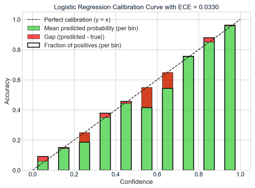
• XGBoost provides the best calibration (ECE = 0.0117) compared with Random Forest (ECE = 0.0475, overconfidence) and logistic regression (ECE = 0.0330, despite low accuracy).
• Predictive entropy highlights that correct predictions tend to lie close to zero entropy, whereas misclassifications happen at higher entropy values (e.g., 0.4–0.7 in the case of logistic regression.

The rest of the paper is as follows. Section 2 will cover the methodological approach and the prediction models. Empirical findings are presented in Section 3, while Section 4 covers the discussion of he results. The conclusion is covered in Section 5.

2. Methodology

This section describes the methodological framework employed to meet the study’s key aim to explore the extent to which explainable AI and uncertainty quantification can improve both the interpretability and trustworthiness of credit risk prediction. These selections are shaped by a lack in the literature, where predictive performance is traditionally emphasised, and interpretability and uncertainty are deprioritised. In the study, three models were used—logistic regression, Random Forest, and XGBoost—chosen for their ability to identify nonlinearities and for predictive accuracy. The combined methods enable analysis of whether greater complexity comes at the expense of interpretability and reliability. The SHAP and LIME were chosen as complementary explainability approaches because they give both global and local insights into model performance. Entropy and Expected Calibration Error were calculated to evaluate uncertainty and assess probability estimation accuracy. Together, these choices provide a solid foundation for an integrated analysis of predictive performance, interpretability and uncertainty in credit risk modelling.

2.1. Data Source

The study is based on the HMEQ dataset, which consists of 5960 U.S. home equity loan applicants and documents borrower characteristics and delinquency results. These data are publicly available at https://www.listendata.com/2019/08/datasets-for-credit-risk-modeling.html?m=1 (accessed on 13 February 2025).

2.2. Data Preprocessing

The dataset was preprocessed and cleaned prior to model training to prepare it for credit risk analysis, using appropriate domain-specific preprocessing steps. As for numerical features, such as MORTDUE, VALUE, YOJ, DEROG, DELINQ, CLAGE, NINQ, CLNO, and DEBTINC, they were imputed as means. On the other hand, in this case, the most frequent category was used to represent categorical features (REASON, JOB, etc.) in the model. For the BAD target variable (bad), due to class imbalance (default vs. non-default cases), the synthetic minority over-sampling technique (SMOTE) was applied to the training set, producing synthetic examples of the minority class to obtain a balanced dataset model training. We one-hot encoded important categorical variables, including REASON (e.g., HomeImp) and JOB (e.g., Other, Office, Sales, Mgr), to represent them numerically for classification modelling. These preprocesses helped ensure that the dataset was complete, fair, and formatted correctly, to the degree that it was made replicable, thereby improving credit risk detection and prediction reliability.

2.3. Model Development Workflow

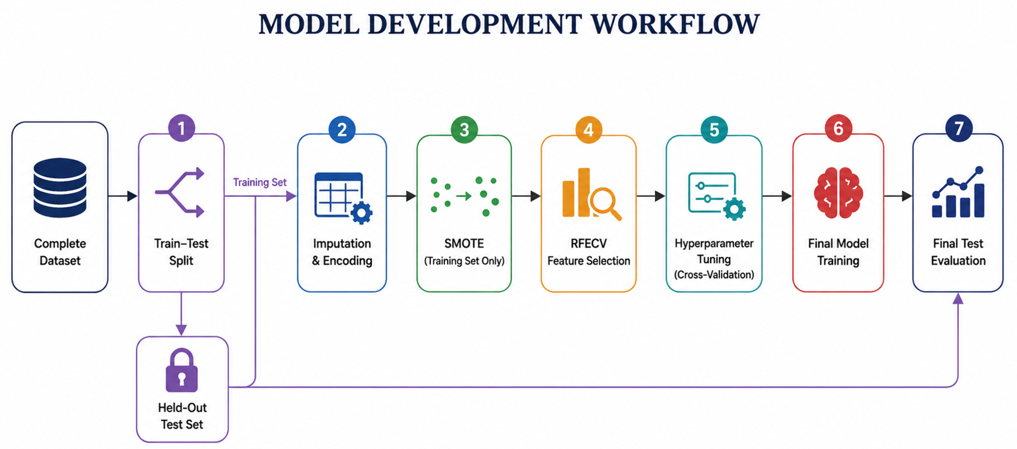
Figure 1 presents the overall model development workflow adopted in this study. To prevent data leakage, the dataset was first divided into training and testing subsets. All preprocessing, class balancing, feature selection, and hyperparameter optimisation procedures were performed exclusively on the training data, while the test set was reserved for final model evaluation.

2.4. Models

The next section describes three loan default prediction models used in this study. It follows each model in detail—the background principles, the operational mechanics, and its application to the dataset across different categories—to help identify defaulters from non-defaulters.

2.4.1. Random Forests

Random Forest (RF) derives from the results obtained from prior work for the decision tree approach. The basis for RF was established with decision trees for statistical classification in Breiman and Ihaka (1984), which introduced decision trees as a statistical classification method, whereas Breiman (2001) built upon this by proposing the RF ensemble learning method. The RF method combines two of the early methods—Breiman’s bootstrap aggregating (bagging) and Ho’s random subspace method—and is built through three successive steps (Breiman 1996; Ho 1998).

Bagging produces m distinct training samples, denoted as $S_j$ for $j=1,2,\dots ,m$, each drawn with replacement from the original dataset and containing the same number of observations as the full dataset. The random subspace method is then applied to construct m decision trees from these samples, represented as $\{f(Z,{\mathrm{\Phi }}_j),j=1,2,\dots ,m\}$, where Z is the feature vector for classification, and ${\mathrm{\Phi }}_j$ is an independent random variable introducing diversity into each tree. The overall prediction is obtained by aggregating the outputs of all m trees through majority voting, expressed as

$$\begin{array}{c}\hfill F\left(z\right)=\arg \underset{C}{\max }{\displaystyle \sum _{j=1}^m}I(f_j\left(z\right)=C),\end{array}$$

(1)

where $F\left(z\right)$ denotes the ensemble’s final prediction for input z, $f_j\left(z\right)$ represents the prediction of the j-th individual tree, C indicates a candidate class label (e.g., default or non-default), and $I(·)$ stands for an indicator function—its value is 1 if the condition holds, 0 in any other case. The expression picks the class C that gets the most votes across the m decision trees.

In credit risk analysis, every decision tree learns from a randomly picked group of borrowers along with a random selection of financial factors. Due to the diversity of these features, the risk of overfitting decreases, while the system can more effectively reflect heterogeneous customer patterns and intricate relationships among financial features (Lessmann et al. 2015). 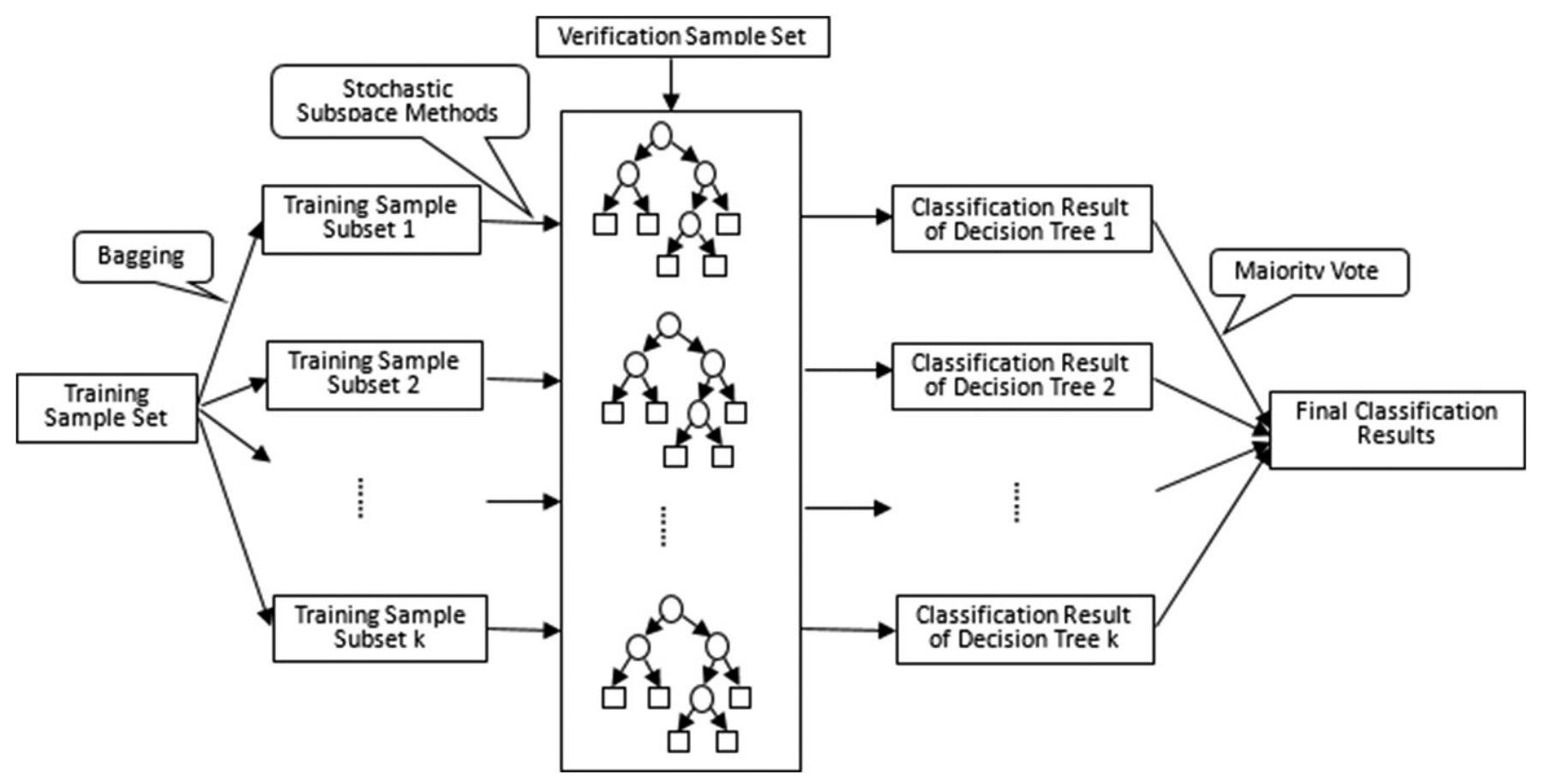Thanks to its combined structure, RF delivers high predictive accuracy and is resilient to noisy, messy data; it is an asset for managing variable, noisy datasets common in predicting loan defaults (Nandipati and Boddala 2024). The operational framework of the Random Forest model used in credit risk assessment is illustrated in Figure 2.

Beyond prediction, RF provides tools for assessing feature relevance, revealing important default risk determinants, and improving clarity (Baesens et al. 2003). Such assessments matter to bankers and supervisors, who want to know what factors, whether debt use, repayment patterns, or borrowing duration, contribute overwhelmingly to the likelihood of default. RF is powerful but may impose a heavy computational burden on large datasets, and its structure is not as clear as that of simpler methods like LR (Nwafor et al. 2024). RF is, however, still prevalent in today’s credit scoring systems because of its high accuracy-to-consistency ratio.

2.4.2. Extreme Gradient Boosting

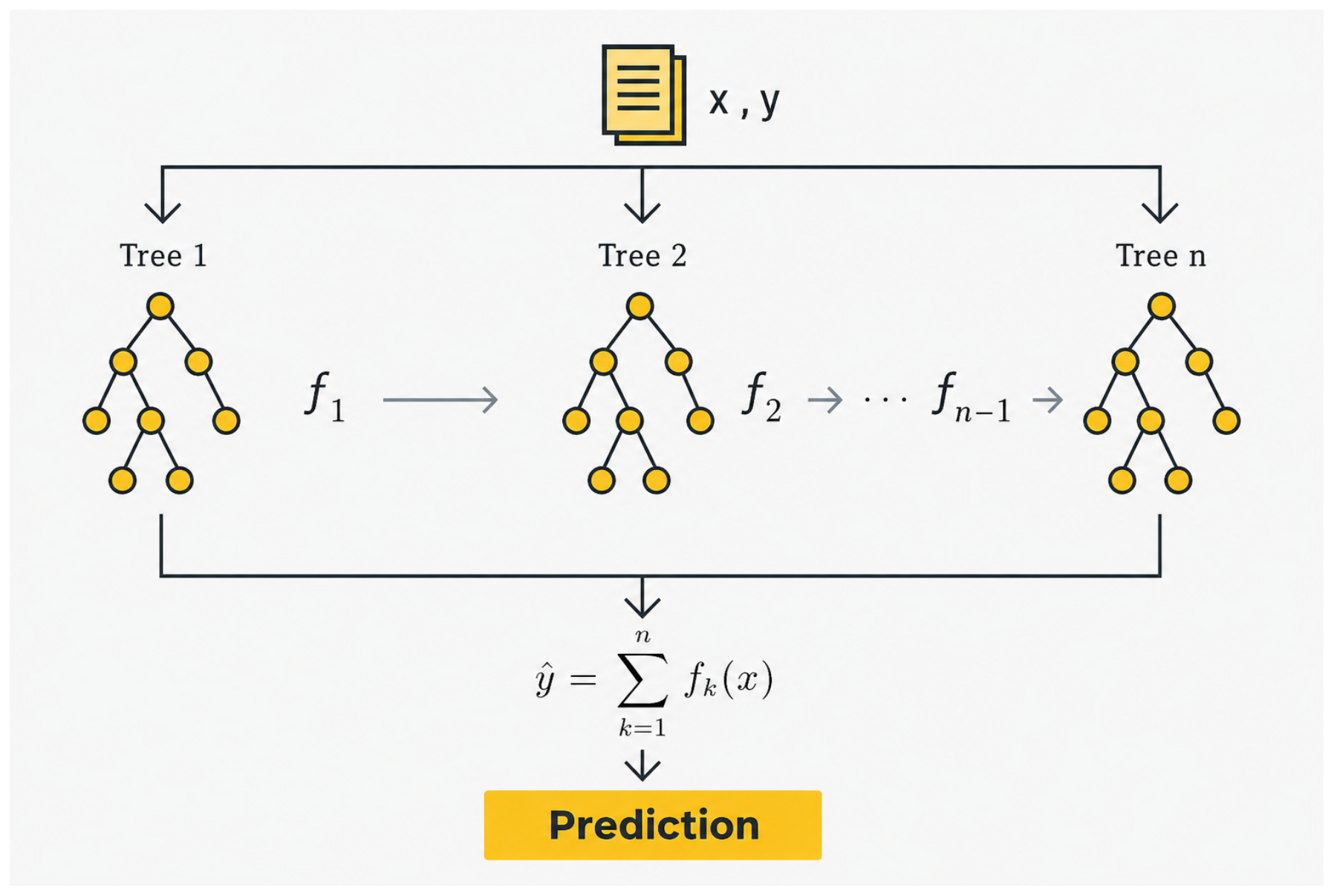
Extreme Gradient Boosting (XGBoost) optimises standard gradient boosting by using gradient descent and second-order Taylor expansions that increase speed and accuracy (Alagic et al. 2024; Zhao et al. 2022). Instead of working in isolation, trees are progressively integrated, each correcting the errors from before. In this environment, new models target errors that have not yet been exploited. The update is performed in a sequential, adaptive manner; hence, the method achieves high performance in classification, forecasting, and ordering problems. Where RF relies on vote-based outcomes, this system aggregates outputs via weighted tree contributions (shown in Figure 3):

$$\begin{array}{c}\hfill {\widehat{y}}_i={\displaystyle \sum _{m=1}^M}{g}_m\left(w_i\right),g_m\in \mathcal{G},\end{array}$$

(2)

where $\mathcal{G}$ is the set of tree-like functions, $g_m$ is a tree, $g_m\left(w_i\right)$ is a result from the i-th tree, and ${\widehat{y}}_i$ is the forecasted value for input $w_i$.

XGBoost is a tree-based system for large-scale ML processes. Since it performs well across many human applications, data scientists widely use it (Chen and Guestrin 2016). Rather than strictly fitting the data, the strategy employs a penalised objective that balances error with complexity to prevent overlearning. It constructs trees incrementally via gradient boosting, with a quadratic approximation for a faster update rate (Alagic et al. 2024; Alkhyeli 2023).

The objective function which XGBoost seeks to minimise is given by

$$\mathcal{O}\left(\psi \right)=\mathcal{C}\left(\psi \right)+\mathcal{P}\left(\psi \right),$$

where $\mathcal{C}\left(\psi \right)={\sum }_{n=1}^{N}L(a_n,{\widehat{r}}_n)$ is the cost function that measures the difference between the predicted outcome ${\widehat{r}}_n$ and the observed value $a_n$, and $\mathcal{P}\left(\psi \right)={\sum }_{j=1}^J\mathcal{P}\left(f_j\right)$ is a regularisation feature that constrains structural complexity. The learning algorithm works with iterative augmentation. For instance, since ${\widehat{r}}_n^{\left(j\right)}$ is defined as the output of the n-th sample at the j-th stage, the iterative update looks exactly like this:

$${\widehat{r}}_n^{\left(j\right)}={\widehat{r}}_n^{(j-1)}+f_j\left(z_n\right).$$

XGBoost was used in this study because (Wang et al. 2022). It is effective in credit scoring, and the prediction accuracy is balanced by XGBoost’s simplicity (Wang et al. 2022). Its gradient-boosting structure enables the detection of subtle patterns in borrowing behaviour, and its built-in regularisation further improves reliability on fresh data (Ali et al. 2023).

2.4.3. Logistic Regression

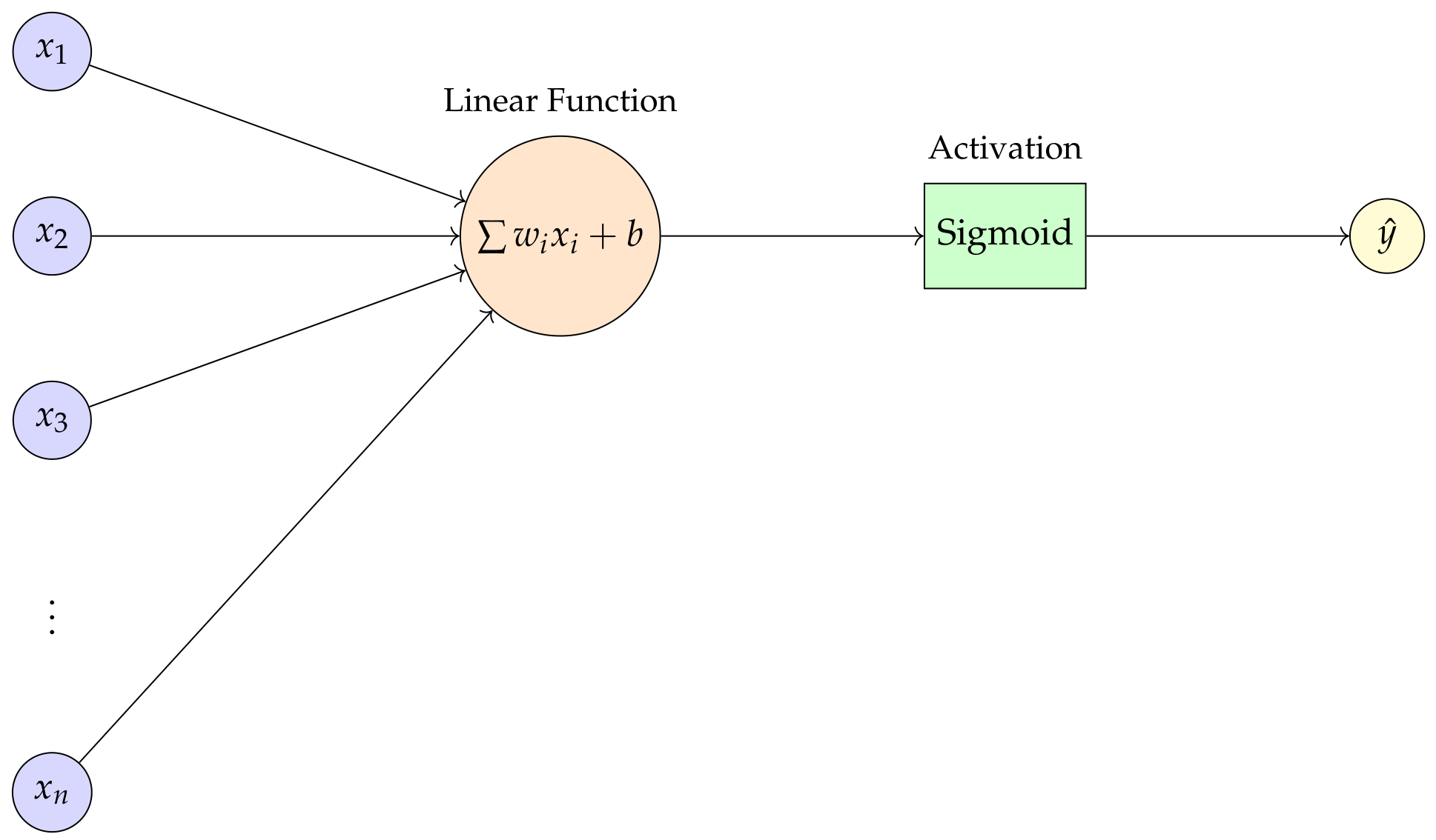
Logistic regression (LR) is used as a baseline method because it is good at learning the values when two outcomes are observed (Musa 2013). LR takes weighted inputs and transforms them into values between 0 and 1 that represent probabilities, rather than summing them. The parameters are estimated using maximum likelihood, which selects values that maximise the probability of producing the observed data without loss of statistical validity. Unlike sophisticated models, LR provides much more certainty; its coefficients indicate the degree—and direction—of the influence of various factors on the produced result (Šarlija et al. 2017). This interpretability benefits LR in applications that depend heavily on explainable decisions, which is a very important issue in supervised systems. Stable, consistent, and easy to use, logistic regression is the basis for more advanced methods. The process for its use is presented in Figure 4.   

2.5. Model Development and Implementation

The model used for this study is a supervised machine learning model trained on a dataset of explanatory variables and corresponding labels. The dataset was divided 80/20 for training and testing. The training dataset was used to train three algorithms, XGBoost, RF, and LR. Hyperparameters were tuned with a 5-fold cross-validation grid search, and the hyperparameters that yielded the best ROC-AUC performance were selected. Model selection is based on ROC-AUC, F1-score, ECE, computational efficiency, and the interpretability of the three models. The process was established to ensure the predictive accuracy of the models used in model selection and reliability in estimating probabilities and realism; reasonable guidance for the practical decisions of credit risk assessment is obtained, which is done to ensure the correct risk prediction of the chosen model as well as to confirm its reliability of model with the realistic model predicting the probability estimation with high probability and in a reasonable manner.

2.6. Integrated Evaluation Framework

The framework presented here is an experimental pipeline for credit risk assessment that combines predictive modelling, explainability estimation with predictive analysis, probability calibration, and uncertainty estimation into a single experiment to measure the predictive risk of a credit variable. Integration here refers to the operationalised evaluation of these components within the same train–validation–test framework, rather than as isolated post hoc analyses.

Following model training and prediction, SHAP and LIME are employed to assess global and local feature contributions; Expected Calibration Error (ECE) is applied to assess confidence in expected probabilities at the portfolio level; and entropy-based measures are used to measure instance-level predictive uncertainty. The framework offers a more holistic evaluation of model performance, explaining behaviour, calibration quality, and uncertainty estimates as metrics for credit risk prediction.

2.7. Explainable AI Approaches

2.7.1. Local Interpretable Model-Agnostic Explanations

LIME helps explain how ML models make decisions—making their outputs easier to understand. Introduced by Ribeiro et al. (2016), it tackles the issue of opaque models that act like “black boxes.” Rather than analysing the entire system, LIME focuses on a single prediction at a time. For each case, it builds a simpler model near that specific input point. By slightly tweaking the inputs, it gathers predictions from the original model on the modified examples. Then, using those results—with more weight given to similar cases—it trains a transparent approximation (Gramegna and Giudici 2021). The surrogate model subsequently identifies the features that had the greatest impact on the prediction. For a given instance x, the LIME explanation is defined as (Gramegna and Giudici 2021)

$$\varphi \left(x\right)=\arg \underset{g\in \mathcal{G}}{\min }\mathcal{L}(M,g,w_x)+\mathcal{C}\left(g\right),$$

(3)

where

• $M:{\mathbb{R}}^p\to \mathbb{R}$ is the black box model,
• $\mathcal{G}$ is the set of interpretable surrogate models;
• $g\in \mathcal{G}$ is a candidate surrogate;
• $w_x\left(z\right)$ is a proximity kernel giving higher weight to points z near x;
• $\mathcal{L}(M,g,w_x)$ is the locality-weighted loss, measuring how well g approximates M locally;
• $\mathcal{C}\left(g\right)$ is a complexity penalty to ensure interpretability.

LIME explanations were generated for the same instances using the lime_tabular module with default parameters to compare local fidelity.

2.7.2. Shapley Additive Explanations

SHAP is a unified framework for interpreting machine learning model predictions based on game theory. Introduced by Lundberg and Lee (2017), it connects several existing explanation methods and provides a solid theoretical foundation using Shapley values from cooperative game theory. SHAP gives each feature a “Shapley value”, which represents its average marginal contribution to a given prediction across all possible feature combinations. This measures how much Shapley moves per feature (from the base value or average prediction), spreading the prediction across features and yielding local and global explanations for this feature parameter (Ariza-Garzón et al. 2020). The SHAP value for feature i is mathematically defined as (Gramegna and Giudici 2021)

$${\varphi }_i=\sum _{S\subseteq F\setminus \left\{i\right\}}{\displaystyle \frac{\left|S\right|!\left(\right|F|-|S|-1)!}{\left|F\right|!}}\left[f(S\cup \{i\left\}\right)-f\left(S\right)\right],$$

(4)

where S is a set of features excluding i, F is the set of all features, and f is the model prediction function. Some key features and benefits of SHAP values are:

• Local accuracy: sum of all SHAP values is equal to the difference between the model’s prediction and the average prediction.
• Missingness: variables absent from the model get a SHAP score of zero.
• Consistency: shifting a model so that one feature impacts the outcome more, the value of SHAP stays the same, or goes up.

Model-agnostic responses were produced for the test set. Using the SHAP library, SHAP values were calculated with KernelExplainer for global interpretability and single-case treatment.

2.8. Quantifying Prediction Uncertainty

UQ is the evaluation of the dependability of the prediction by a model. Developing predictive systems—particularly in high-stakes cases like credit scoring—cannot just be about getting the right answer; it is also about the level of confidence that supports it. The devil-may-care approach to predicting with confidence only increases the overall accuracy (Habibpour et al. 2023) and underlines how important it is that people stay informed and not trust a single AI model (Habibpour et al. 2023).

2.8.1. Entropy for Uncertainty Quantification

Entropy indicates the degree of uncertainty for a probability distribution. Predictive entropy is also known as data entropy. Shannon first developed it in information theory (Shannon 1948) for randomness in data. For machine learning problems, predictive entropy (PE) is used to determine whether a model is certain about its output (Habibpour et al. 2023). PE for two-class problems ($j=2$) can be written as

$$PE=-{\displaystyle \sum _{j=1}^2}{p}_j\log p_j,$$

(5)

in which $p_j$ is the estimated confidence level on class j (default or non-default). PE scores tend to decrease with certainty and increase with unpredictability. Uncertainty declines as the outcome becomes more certain, reaching zero when the prediction is entirely certain. Predictive entropy was computed for test set predictions. The credit risk analysis entropy helps to determine the performance of default probability estimates (Li and Chen 2021). With unseen outcomes, specialists can zero in on uncertain cases by requesting additional data or adjusting how the evaluation is assessed. In high-uncertainty scenarios, it is important to seek alternative processes rather than relying solely on model outputs. Highlighting that unpredictability yields better choices, minimising mistakes in risky candidate classification, and bolstering scoring models.

2.8.2. Model Calibration

Model calibration is the adjustment of the models to make such predictions consistent with the world as observed (Habibpour et al. 2023). In credit risk, precise PD prediction depends on considering actual default rates to facilitate loan selection. However, even the best model of segmented, risky, and safe borrowers might well still be incorrect in its probability scores and produce misguided verdicts. We can assess calibration by ECE, an evaluation that demonstrates the distance between predictions and actuals across a set of associated probability ranges (Wang 2023).

$$ECE={\displaystyle \sum _{k=1}^K}{\displaystyle \frac{|S_k|}{T}}\left|{\overline{y}}_k-{\overline{p}}_k\right|,$$

(6)

This formula uses $S_k$ for the predictions in bin k and $|S_k|$ for the number of cases in that bin. Here, T is the sum of all predictions. Calibration was verified by splitting the predictions into 10 ’equal-width’ bins and computing the ECE. The value ${\overline{y}}_k$ shows the actual percentage of positive results in bin k. The value ${\overline{p}}_k$ represents the average predicted probability occurring in the same bin. A well-calibrated model yields known, well-formed, and trusted probabilities, which help us to make better risk decisions. In addition, calibration reflects entropy-based uncertainty measures, where the confidence a model has in its estimates of default probabilities aligns with what was actually observed.

2.8.3. Calibration and Predictive Uncertainty as Distinction

Calibration is different from prediction uncertainty. Calibration assesses the population- or group-level reliability of predicted probabilities and how well predicted risk scores match observed outcome frequencies. On the other hand, predictive entropy represents uncertainty at the instance level by describing the uncertainty associated with a single prediction within the context of the probability distribution. Calibration tells us how closely predictions align with observations, and entropy specifies how much uncertainty there is in the probability associated with any given prediction. Hence, there are analogous but not equal roles for calibration and entropy in credit risk prediction.

2.9. Performance Evaluation

2.9.1. ROC and AUC

The ROC curve plots TPR vs. FPR for different threshold settings. An AUC score is a single value; 1.0 indicates good prediction, and 0.5 is chance-level performance, indicating that sensitivity offsets specificity. In mathematical terms:

$$\begin{array}{cc}\hfill \mathrm{TPR}\left(\mathrm{Recall}\right)& ={\displaystyle \frac{\mathrm{TP}}{(\mathrm{TP}+\mathrm{FN})}}\hfill \\ \hfill \mathrm{FPR}& ={\displaystyle \frac{\mathrm{FP}}{(\mathrm{FP}+\mathrm{TN})}}\hfill \end{array}$$

ROC AUC validates unbalanced classes because performance is evaluated through several thresholds instead of just one. Cutoffs differ, and a wider range provides a cleaner view.

2.9.2. F1-Score

The F1-score is a common metric for binary classification with imbalanced class distributions. The precision and recall are then averaged using the harmonic mean and adjusted for Type I and Type II errors.

$$\begin{array}{cc}\hfill \mathrm{Precision}& ={\displaystyle \frac{\mathrm{TP}}{(\mathrm{TP}+\mathrm{FP})}}\hfill \\ \hfill \mathrm{Recall}& ={\displaystyle \frac{\mathrm{TP}}{(\mathrm{TP}+\mathrm{FN})}}\hfill \\ \hfill \mathrm{F}1-\mathrm{Score}& =2\times {\displaystyle \frac{\mathrm{Precision}\times \mathrm{Recall}}{(\mathrm{Precision}+\mathrm{Recall})}}\hfill \end{array}$$

A value of 1 indicates high accuracy in recall and precision, but near zero indicates weak results. This is pertinent when the impact of wrong predictions—whether positive or negative—differs from that of right predictions.

3. Empirical Results and Discussion

3.1. Dataset Description

The HMEQ dataset, which consists of 5960 home equity loan requests, was utilised in this study. The loan is secured by the property and is based on its value. The dataset comprises applicant attributes and loan factors (delinquency history, amount loaned, level of earnings, tenure at job, credit history, and whether a default occurred). A few variables are given in

Table 2. (a) Credit Risk Dataset—Sample Records. (b) Description of Variables.

(a)
Bad	Loan	Mortdue	Value	Reason	Job	Yoj	Derog	Delinq	Clage	Ninq	Clno	Debtinc
0	1700	97,800	112,000	HomeImp	Office	3	0	0	93.33	0	14	NaN
1	1700	30,548	40,320	HomeImp	Other	9	0	0	101.47	1	8	37.11
1	1800	48,649	57,037	HomeImp	Other	5	3	2	77.10	1	17	NaN
(b)
Variable			Description
Bad			Loan default status: 1 = defaulted or seriously delinquent; 0 = otherwise
Loan			Loan amount requested
Mortdue			Balance on existing mortgage
Value			Current property value
Reason			Purpose of the loan (DebtCon = debt consolidation; HomeImp = home improvement)
Job			Occupation type
Yoj			Years in current job
Derog			Number of major derogatory credit reports
Delinq			Number of delinquent credit lines
Clage			Age of oldest credit line
Ninq			Number of recent credit inquiries
Clno			Total number of credit lines
Debtinc			Debt-to-income ratio

(a); explanations for various variables are provided in Table 2(b).

3.2. Software and Packages

The application of Python in this study is based on its flexibility, user friendliness, and its strong well-established validation of its applications within the data science and ML environments. Analyses were run on Python 3.x, which is widely used with popular stats and ML tools. Pandas is a top-level module in NumPy that handles data processing and cleaning. Visuals are written using Matplotlib version 3.10.8 and Seaborn version 0.13.2. There is a lot of reliance on scikit-learn modelling methods, such as LR, RF, and XGBoost. LIME and SHAP are seen as XAI techniques for improving clarity and providing uncertainty measures. Together, this is a sound approach for credible and interpretable credit risk evaluation.

3.3. Exploratory Data Analysis

In this section, we present initial data interpretations. In a large dataset, only the key features need to be closely examined. Rather than a data structure, we observe the general characteristics of the data. Separately, the experiment looks at the dependent variable to determine how it spreads or behaves. We also highlight the most clear trends and core takeaways of the review.

Check the data completion before analysis. For numerical data,

Table 3. Descriptive Statistics and KS Values.

Var	Mean (All)	SD (All)	Mean (ND)	SD (ND)	Mean (D)	SD (D)	KS
LOAN	18,607.97	11,207.48	19,028.11	11,115.76	16,922.12	11,418.46	0.1386
MORTDUE	73,760.82	44,457.61	74,829.25	43,584.99	69,460.45	47,588.19	0.0955
VALUE	101,776.05	57,385.78	102,595.92	52,748.39	98,172.85	74,339.82	0.1028
YOJ	8.92	7.57	9.15	7.68	8.03	7.10	0.0885
DEROG	0.25	0.85	0.13	0.51	0.71	1.47	0.2249
DELINQ	0.45	1.13	0.25	0.67	1.23	1.90	0.3216
CLAGE	179.77	85.81	187.00	84.47	150.19	84.95	0.2192
NINQ	1.19	1.73	1.03	1.53	1.78	2.25	0.1591
CLNO	21.30	10.14	21.32	9.68	21.21	11.81	0.0735
DEBTINC	33.78	8.60	33.25	6.95	39.39	17.72	0.2648

displays summary statistics of the whole sample as well as various definitions for borrowers who did not default (ND) and those who defaulted (D) as a basis step. It includes the mean and standard deviation rather than simply the average. Differences between the ND and D groups are summarised using a single-column Kolmogorov–Smirnov (KS) statistic. This suggests a degree of separation between the distributions, with higher values indicating significant separating power for lending risk. Defaults usually mean more overdue payments, lower credit ratings, higher debt-to-income ratios, and less time spent building a credit history. The average number of late payments is 1.23 for default points, 0.25 for others, and 0.71 for negative records (vs. 0.13). By default, the debt-to-income ratio is 39.39%, whereas for non-defaulting borrowers, it is 33.25%. The average credit history duration is 150 months for debt default and 187 months for debt without default. The KS scores they each display are quite high, indicating a clear separation between the two groups.

Non-defaulting people have more stable finances (so they are not likely to default), which ties in nicely with the conclusion that timely payments, reasonably large debt, and established credit records reduce default risk. In contrast, items such as borrowing amount, home value, employment, total accounts, and outstanding mortgage loans indicate weaker differential and lower KS scores, reflecting little predictive power for default.

Table 4. Categorical Variables and Default Rates.

Category	Relative Frequency	Default Rate	Chi2 p-Value
REASON: DebtCon	0.6591	0.1897	0.004576
REASON: HomeImp	0.2987	0.2225	0.004576
JOB: Mgr	0.1287	0.2334	$3.3067\times {10}^{-16}$
JOB: Office	0.1591	0.1319	$3.3067\times {10}^{-16}$
JOB: Other	0.4007	0.2320	$3.3067\times {10}^{-16}$
JOB: ProfExe	0.2141	0.1661	$3.3067\times {10}^{-16}$
JOB: Sales	0.0183	0.3486	$3.3067\times {10}^{-16}$
JOB: Self	0.0324	0.3005	$3.3067\times {10}^{-16}$

shows that default levels differ among REASON and JOB types. Using a Chi-square test rather than assuming independence, we examined the connections between these categories and the outcome. When people took loans for future home improvements (HomeImp), they defaulted more frequently—22.25%—than when people paid off old loans (DebtCon) with 18.97%. In occupations, defaults are highest for Sales (34.86%) and Self-employed (30.05%), while Office and ProfExe have lower default rates (13.19% and 16.61%). This indicates that loan status and occupation are among the leading predictors of default risk.

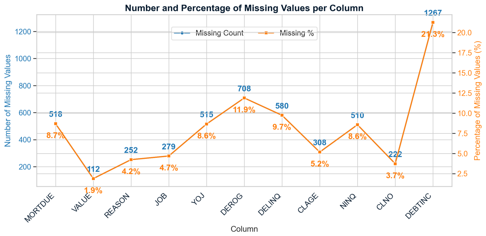
Figure 5 provides both the percentage and number of missing values for several variables aside from the ones with total observations. For instance, supervised learning techniques like RF can handle missing values, but NNs typically require fully observed data to perform well (Berendsen 2019). The variable DEBTINC shows the highest proportion of missing data (21.3%), followed by DEROG (11.9%) and DELINQ (9.7%).

As a result, appropriate imputation techniques were applied to ensure data completeness. The detailed approach to handling missing values is described in Section 3.4.1.

The target variable, symbolised by B, indicates whether a borrower has defaulted on a loan. It is defined as

$$B=\left\{\begin{array}{cc}0,\hfill & \mathrm{for}\mathrm{non}\text{-}\mathrm{default}\mathrm{cases},\hfill \\ 1,\hfill & \mathrm{for}\mathrm{default}\mathrm{cases}.\hfill \end{array}\right.$$

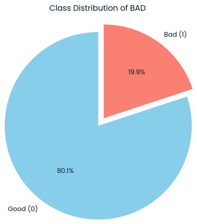
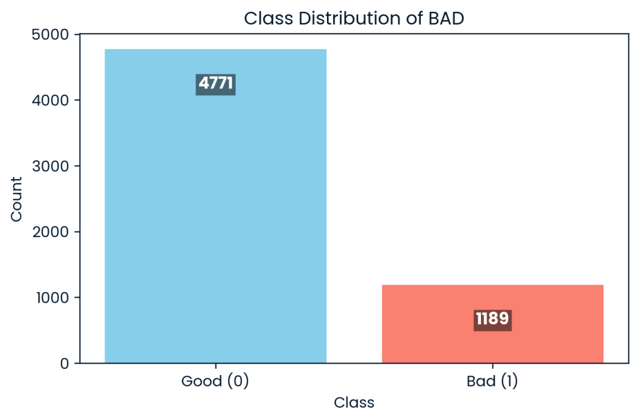
The outcome variable takes only two possible values, indicating that the task at hand is a binary classification problem. The dataset comprises 5960 loan records, of which 1189 (19.9%) represent defaults and 4771 (80.1%) represent non-defaults, as represented in Figure 6 and Figure 7, which illustrate the class distribution using a pie chart and a histogram, respectively.

This reflects a considerable class imbalance, which may bias model training towards the majority class. The imbalance suggests that standard classifiers may perform poorly in identifying the minority (default) cases. To mitigate this, the SMOTE was applied to the training data, as detailed in Section 3.4.3.

3.4. Data Preprocessing

3.4.1. Handling Missing Values

Gaps are common in real-world data; they can also affect the effectiveness of algorithms. To achieve reliable results without sacrificing entry quality, incomplete entries were handled differently; numbers and categories were treated separately. For the numeric columns, the gaps were plugged with the column’s mean. In this way, the total data centre remains intact—no records should be removed. Specifically, for the case of any missing entry $y_i$ in numeric variable y, it was replaced with

$$y_i={\displaystyle \frac{1}{k}}{\displaystyle \sum _{j=1}^k}{y}_j,$$

where k is the number of non-missing values in the column. For categorical factors, missing values were imputed using the mode for each variable. Using only existing levels, it prevents spurious groups from forming and preserves the natural spread of the data.

3.4.2. Encoding Categorical Variables

Categorical variables were converted to numerical values in a one-hot format after filling in missing data. This method would set a yes-or-no flag for each group; however, it does not include a flag for each variable due to overlap. The outcome maintains all original semantics, which makes it usable for an algorithmic model.

3.4.3. Class Imbalance Correction Implemented Using Synthetic Minority Over-Sampling Approach

The experiment we pursued was visibly asymmetric, taking one group as a mere minority of the entire sample. Directly matching classifiers to skewed data often focuses on the larger set, thereby eroding detection of rare outcomes (e.g., defaults). The SMOTE proposed by Chawla et al. (2002) was then adopted to artificially manipulate and balance the background dataset. Using SMOTE, a step is taken that linearly interpolates existing minority samples with their nearest neighbours in the feature space to produce synthetic minority instances. For every particular minority sample $x_i$, one of its closest neighbours $x_{zi}$ is randomly selected, and a new synthetic object is created along lines of the following formula:

$$x_{\mathrm{new}}=x_i+\delta (x_{zi}-x_i).$$

(7)

This is an example of $\delta \sim U(0,1)$, where $\delta \sim U(0,1)$ means a random variable obtained from a uniform distribution of $[0,1]$. SMOTE generates synthetic minority-class samples without replicating the original data, reducing overfitting while preserving the original distribution. SMOTE was first performed by applying Python’s imblearn library with $k=5$ nearest neighbours only on training folds during cross-validation to prevent data leakage.

The dataset was first divided into training and testing sets using an 80/20 split. To address class imbalance, SMOTE was applied only to the training set. As shown in

Table 5. Class distribution in the training set before and after applying SMOTE.

Class	Before SMOTE	After SMOTE
0 (Majority)	3432	3432
1 (Minority)	318	3432

, the original training set contained 3432 instances of Class 0 and 318 instances of Class 1. After applying SMOTE, the minority class was synthetically over-sampled to 3432 instances, resulting in a balanced training set. The test set was not resampled and retained its original class distribution. Consequently, all performance metrics reported in this study were computed on the original imbalanced test set to ensure an unbiased evaluation of model performance.

3.5. Variable Selection

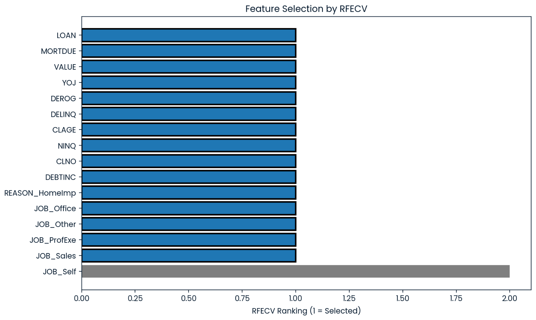
Figure 8 shows the features selected by RFECV based on the RF classifier as an estimator. Through analysis, however, the results show that all features had a positive impact on model performance up to Job_Self, after which it was determined that the feature was non-informative and hence excluded. The remaining predictors were retained and used to fit the final RF model, followed by the evaluation of all other classifiers in that study.

3.6. Supervised Learning Models

This study employs supervised machine learning approaches. In supervised learning, algorithms construct predictive models by learning relationships between explanatory variables and their corresponding target labels from labelled training data. Missing numerical values were imputed using mean imputation, while categorical variables were imputed using the most frequent category. The categorical variables were subsequently one-hot encoded prior to modelling. To address class imbalance, SMOTE resampling was applied with a fixed random seed (random state = 42) to ensure reproducibility.

Following variable selection, the dataset was divided into training and testing subsets using an 80/20 split with stratified sampling and a fixed random seed (random state = 42). Three supervised learning algorithms, namely XGBoost, Random Forest (RF), and logistic regression (LR), were trained using the training data. Hyperparameters for each model were optimised via 5-fold cross-validation with grid search, using shuffling and a fixed random seed to maintain consistent fold assignment across experiments. The optimal parameter combination was selected based on the highest ROC AUC score.

3.6.1. Best Model Parameters

For the XGBoost classifier, the hyperparameters selected through grid search were a learning rate of 0.2, a maximum depth of 7200 estimators, and a subsample ratio of 0.8. For the RF classifier, the optimised parameters were bootstrap = False, max_depth = None, max_features = ‘sqrt’, min_samples_leaf = 1, min_samples_split = 2, and 200 estimators. For LR, the chosen hyperparameters were C = 1, penalty = ‘l1’, solver = ‘liblinear’, and l1_ratio = None. These configurations were used to train the final models and were subsequently evaluated on the test set, ensuring that each model achieved optimal predictive performance while maintaining interpretability and robustness.

3.6.2. Evaluation of Model Performance

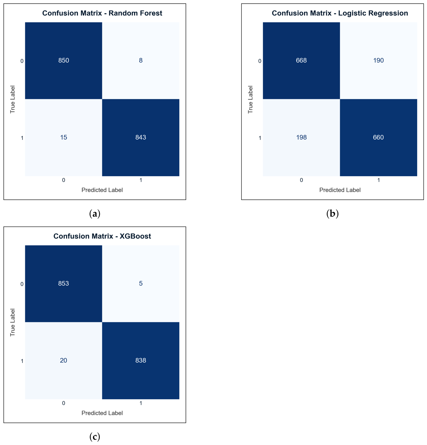
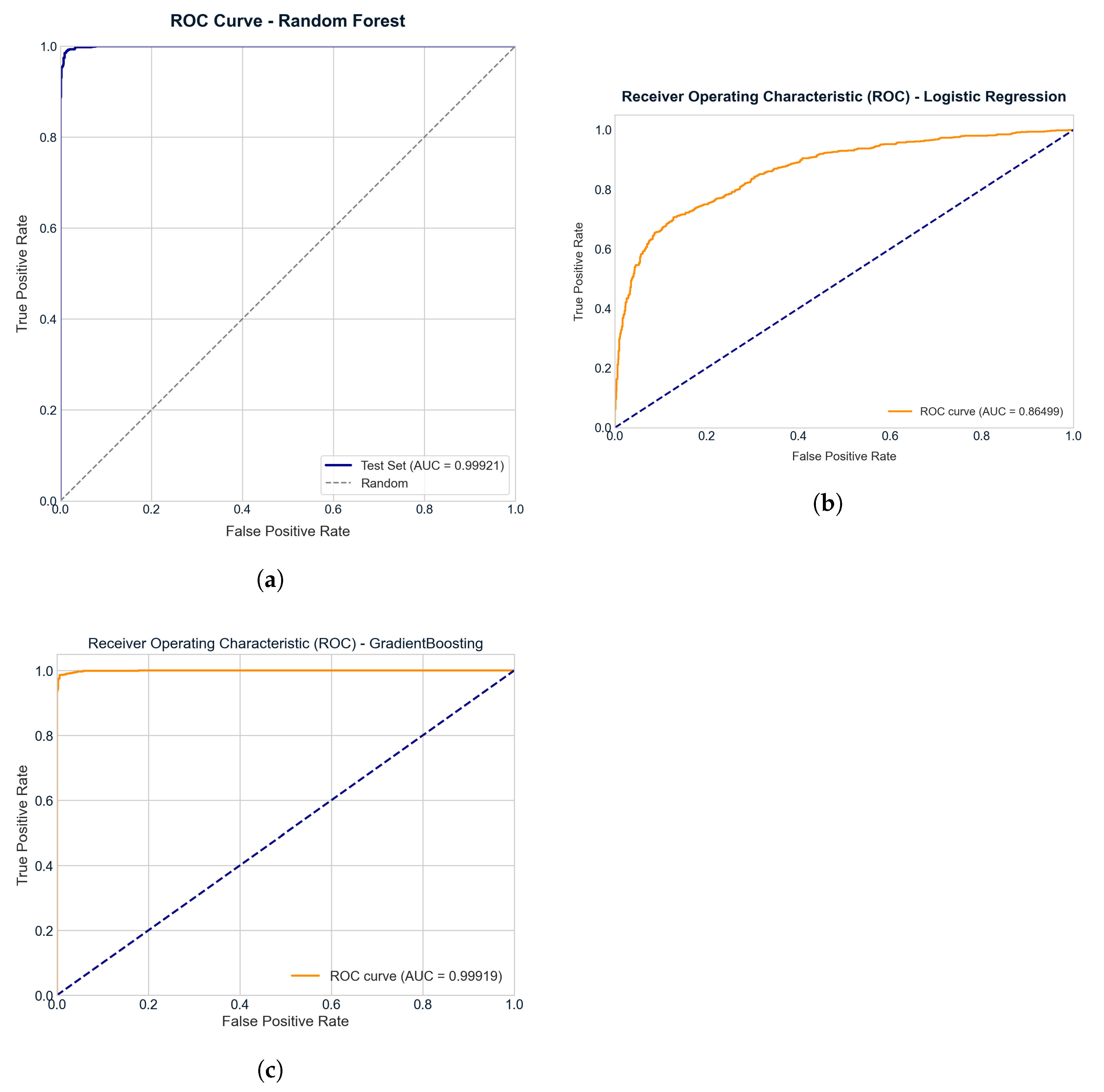
The performance of the classification models, RF, LR, and XGBoost, was quantified using confusion matrices (Figure 9), ROC curves (Figure 9), and standard classification metrics (see

Table 6. Performance metrics for different classification models.

Model	Accuracy	Precision	Recall	F1-Score
Random Forest	0.9866	0.9906	0.9825	0.9865
Logistic Regression	0.7739	0.7765	0.7692	0.7728
XGBoost	0.9854	0.9941	0.9767	0.9853

). This output provides a comprehensive picture of each model’s performance and predictive confidence from the test set.

Figure 9 shows the confusion matrices that are useful for model performance. RF performs well; however, XGBoost achieves high accuracy and few misclassifications. RF accurately identified 850 true negatives and 843 true positives; XGBoost yielded similar results with 853 true negatives and 838 true positives. These results demonstrate that ensemble methods effectively model both default and non-default borrowers (presumably due to their ability to model complex nonlinear relationships in credit data).

LR, however, has difficulty distinguishing between these two groups. The model returned 190 false positives and 198 false negatives, suggesting limitations in its ability to capture complex patterns. Overall model accuracy is lower due to weaker performance in all measures. These differences are illustrated in an ROC curve in Figure 10. RF exhibited an AUC of 0.9992, trailing only XGBoost at 0.9991, indicating almost perfect distinction between defaulted and recoupable loans. LR is 0.8649, suggesting weaker separation and weaker ability to accommodate nonlinear borrower behaviours. While LR might fit basic linear models, it cannot predict defaults as expected for tree-like ensembles.

Table 6 summarizes the model performance. LR fails, RF and XGBoost achieved over 98% accuracy and higher F1-scores above 0.98. XGBoost outperforms at a precision of 0.9941, thus reducing the number of false positives, a vital consideration for credit risk, where approving high-risk borrowers may entail financial loss. LR has both an accuracy of 0.7739 and a score of 0.7728, so it may not accurately reflect the nonlinear relationships in the data. These findings reinforce that ensemble models not only enhance predictive capacity but also increase the robustness of credit risk analysis, ensuring informed lending decisions.

3.7. Explainable AI for Credit Risk Assessment

A complete analysis of model performance needs to be combined with explanation of why the model arrives at specific predictions, providing transparency and trust with respect to the credit risk decisions. In this section, we apply XAI tools, specifically LIME and SHAP, to achieve both global and local interpretability on the trainable tree-based trained models. These findings also indicate that, to increase the practical use of explainable AI (XAI) in financially regulated systems, it is important to account for explanation outputs in a way that makes them documentable and reproducible for auditing purposes elsewhere. In addition to improving interpretability, SHAP and LIME explanations are generated in a fully reproducible manner using fixed random seeds and a controlled model pipeline. All local and global explanation outputs, including feature contribution values and importance rankings, are systematically stored alongside model predictions. This ensures traceability from input features to final model decisions and associated explanations.

3.7.1. Model Explanation for Tree Ensembles Using LIME

Following the establishment of the procedure for generating explanations with the LIME framework, a technical constraint was identified when applying it to the XGBoost and Random Forest classifiers, as LIME is not compatible with models wrapped in a GridSearchCV object. To resolve this issue, both classifiers were retrained using the best-performing hyperparameters from the tuning stage, enabling them to be stored as native LIME-compatible models.

3.7.2. Insights from LIME Explanations

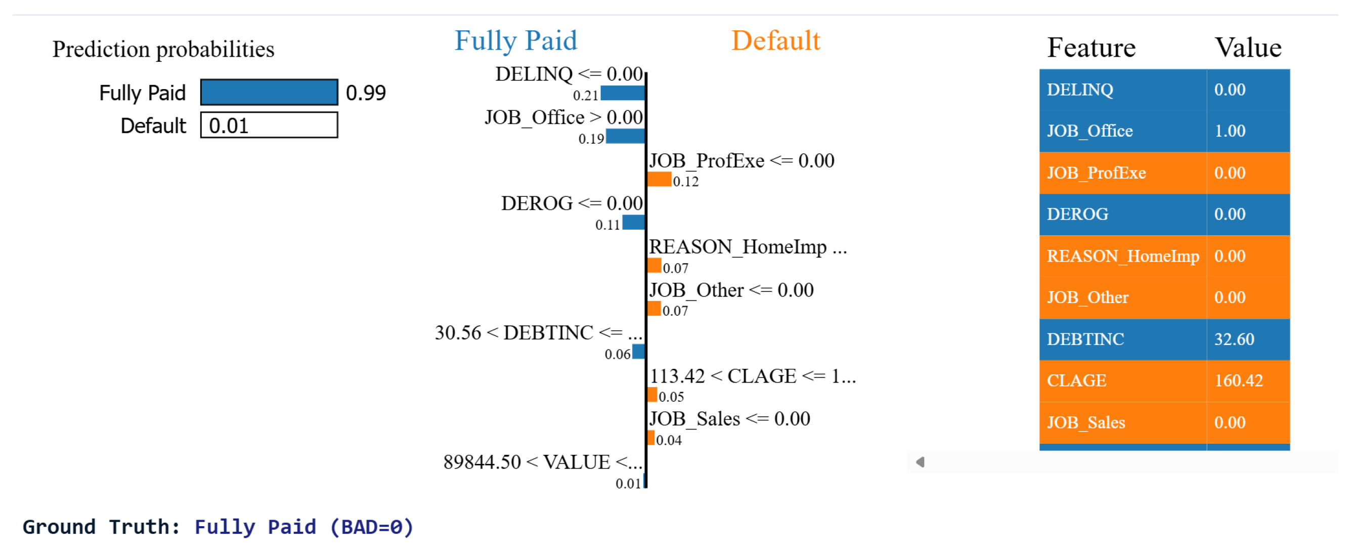
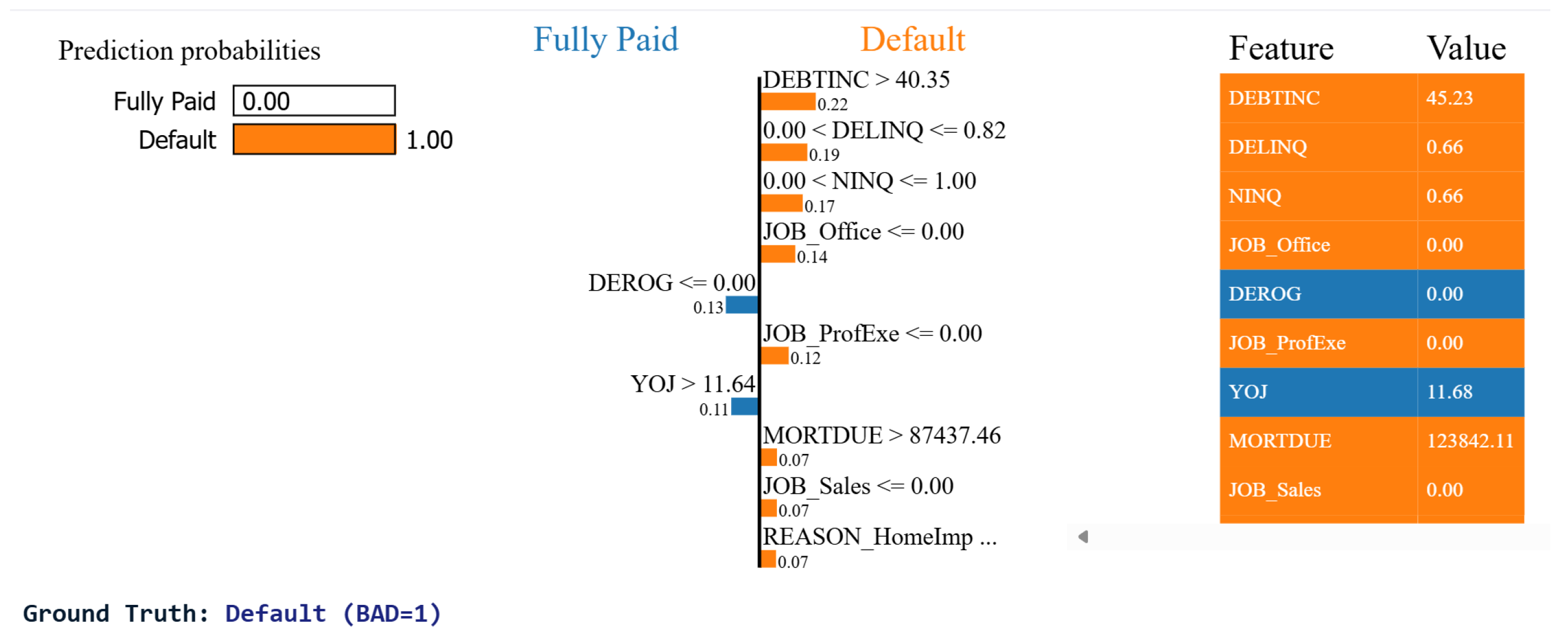
This section presents interpretative insights derived from LIME through three representative case studies. Figure 11 shows a loan predicted as “Fully Paid” (BAD = 0). LIME highlights the top nine factors affecting the outcome, along with their individual impact scores.Two major positive influences appear to be zero delinquencies (“DELINQ = 0”), clean credit documents (“DEROG = 0”), and office occupation (“JOB Office = 1”). These trends are consistent with previous research, indicating that previous payment behaviour and credit cleanliness predict creditworthiness (Rafi et al. 2024).

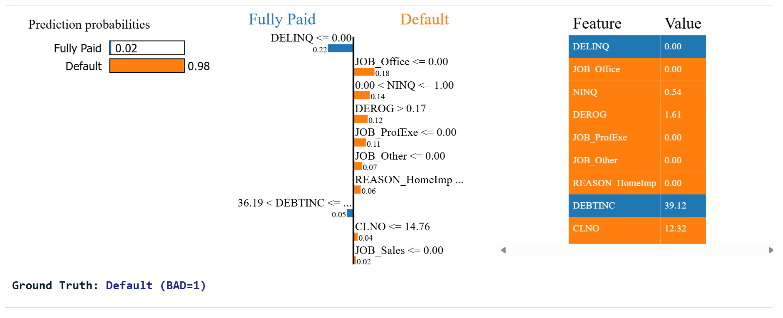
For risky cases (Figure 12), LIME discovers prominent negative contributors with respect to negative legal records, recent credit enquiries and unstable employment. This is consistent with the literature, which shows that high rates of credit applications, prior bad experiences, and employment instability are associated with a higher likelihood of default (Gerardi et al. 2013, 2018). In the XGBoost example (Figure 13), “DEBTINC” and past delinquencies strongly contribute to predicting default. This is corroborated by previous studies using ML and XAI, which show that debt ratios and delinquency counts are both key for predicting default risk (Kim et al. 2018). Taken together, the LIME outputs reveal transparent representations of the effect of each feature on the prediction, which, in part, also confirm known credit-scoring patterns.

3.7.3. Explanation by Global and Local Model Using SHAP

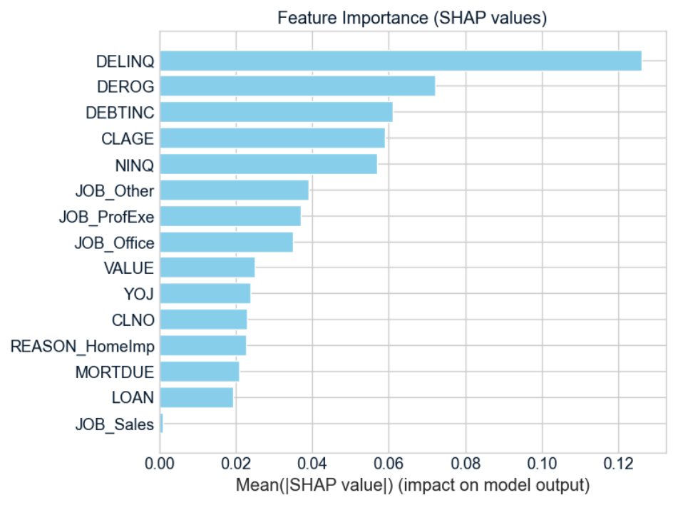
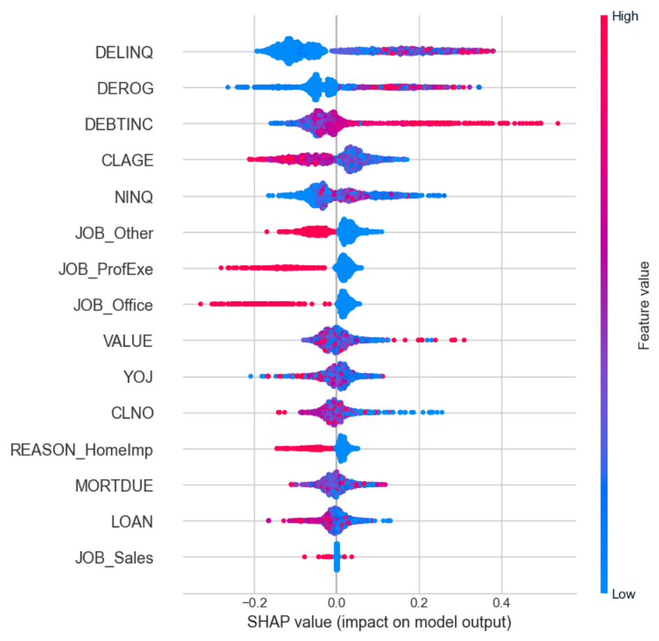
SHAP was used to interpret the models used for trees, both globally and locally. In contrast to LIME, which can also approximate local behaviour, SHAP has exact features in the dataset, according to game principles, to guide interpretations both in direction and intensity. Figure 14 and Figure 15 can summarise those results.

Globally (Figure 14), “DELINQ”, “DEROG”, “DEBTINC” are primary predictors of default. This pattern aligns with empirical credit-scoring results indicating that past delinquencies, derogatory occurrences, and high debt ratios are generally considered important predictors (Rafi et al. 2024).

Directional effects are also visualised using the SHAP summary plot (Figure 15). The higher the value of “DELINQ” and “DEBTINC” (high red points), the more they shift predictions toward default, while the lower the value, the more they push the predictions toward repayment. The employment characteristics show more heterogeneous effects, indicative of income stability across different borrower groups (as suggested by some recent investigations into ML credit scoring (Al Maruf et al. 2024)). In sum, SHAP results support and validate the local results from LIME and show that XAI approaches accurately identify the financial risk factors we know, providing transparency and verification of model performance.

3.8. SHAP and LIME Explanations Compare

To further facilitate the interpretability analysis, the discussion is extended beyond the description of a feature importance to a more informative assessment of explanatory behaviour. Not only do SHAP and LIME help identify core drivers of risk, but they also compare the rankings of the various features, which assess the similarity between the two methods. The main results show robust consistency across the most significant variables, such as DELINQ, DEROG, and DEBTINC, suggesting that local and global explanations yield similar interpretations of model behaviour by focusing on similar underlying financial risk parameters.

Stability of explanation is also investigated by selecting borrowers with similar financial characteristics, which exhibit their feature attributions. Our results show that when we model closely related features, we get similar explanations, meaning the model yields identical responses even when the input data changes slightly. This adds greater confidence to the explanations provided in credit risk applications, which are sensitive to consistency found among such applicants in decision-making.

To understand how predictive uncertainty relates to explanation patterns, we further compare high-confidence and high-uncertainty predictions, which provides additional insight. Usually, high-confidence cases are explained in more detail using SHAP and LIME, focusing on a few features. In high uncertainty situations, feature contributions are less definitive and more scattered. This behaviour is consistent with entropy-based measures of uncertainty and suggests a link with model confidence and interpretability. SHAP and LIME serve to detect the key drivers of financial risk, and both approaches provide consistent explanations under stable operating conditions and meaningful explanations when predictive uncertainty rises.

3.9. Quantifying Predictive Uncertainty

We measure model confidence in default risk prediction failures using predictive entropy, which we use to learn the variation in outcome probabilities, and ECE, which compares average predictions with real-life results. RF introduces inherent variation through bootstrap aggregation, whereas XGBoost and LR contain no such natural stochasticity. Bootstrap resampling was therefore adopted for XGBoost and LR to control for randomness and account for future uncertainty consistently and fairly, thereby improving the performance of all models.

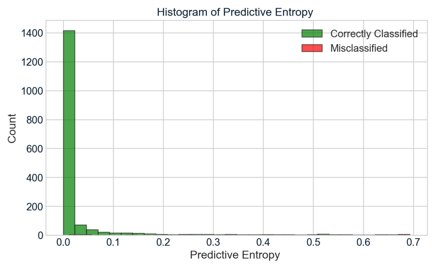
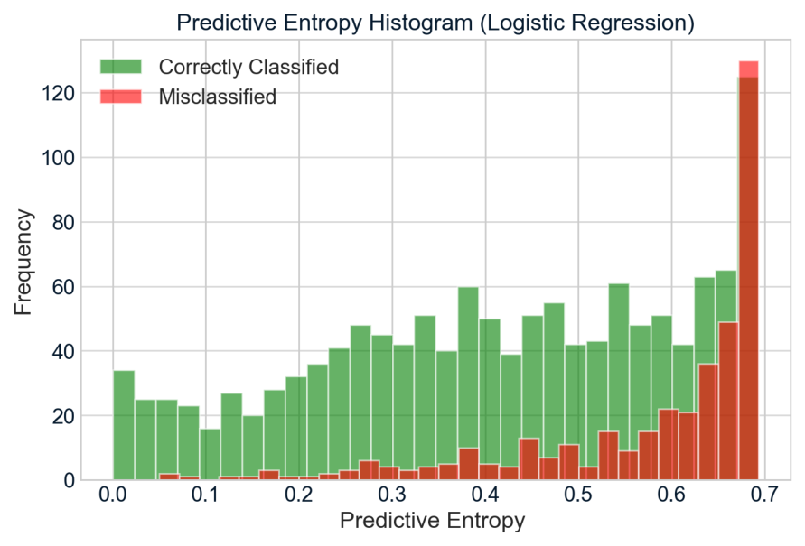
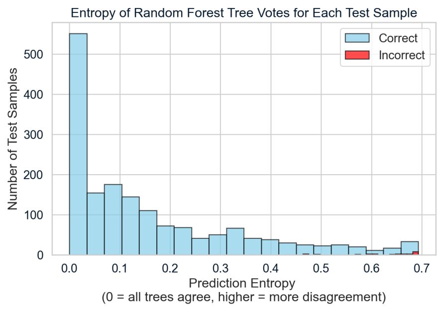
Predictive entropy and model errors appear to exhibit a uniform pattern across all three models; higher uncertainty increases the odds of misclassification. It is evident from Figure 16 that most of the correct predictions made by XGBoost correspond to approximately 1400 samples for which the entropy is near zero, with only a small number of errors occurring where entropy is high, consistent with an accuracy of 98.54%. Figure 17 shows a parallel pattern for RF; when there is high agreement among trees (entropy close to zero), near-perfect accuracy is achieved, and the few errors that occur are concentrated in regions of maximal disagreement. For LR, shown in Figure 18, misclassifications are clustered in the high-entropy region (0.4–0.7), suggesting that although the linear approach is not perfect at separating the underlying data structure (77%), it nevertheless assigns higher uncertainty to challenging cases. These results demonstrate that all three models capture meaningful structure in the data and distinguish confident predictions from ambiguous predictions well. Accuracy differences primarily reflect how effectively each model places samples in the low-entropy “well-understood” domain; LR has a strong linear boundary, whereas XGBoost and RF better capture the underlying nonlinear relationships. Across all models, misclassifications are almost exclusively clustered in high-entropy regions, demonstrating that predictive entropy is an indicator of uncertainty and a very good signal for tentative treatment of predictions.

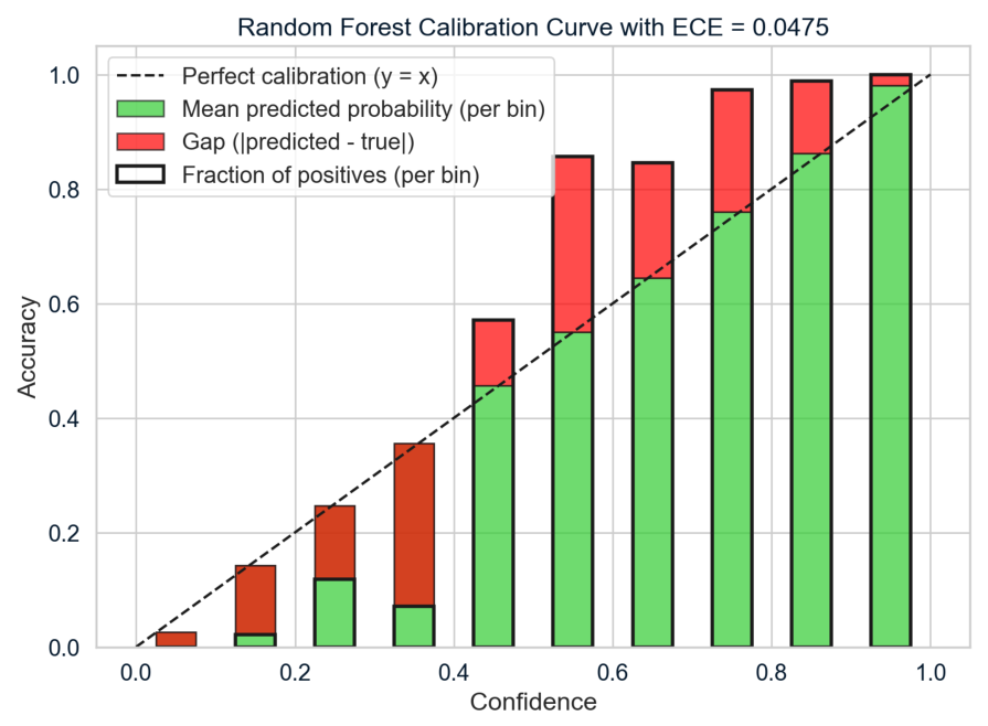
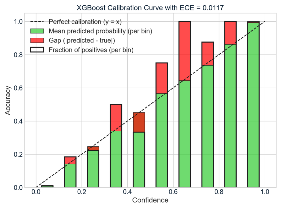
Although RF shows slightly stronger predictive metrics than XGBoost (see Table 6), the difference between the models is minimal. Their calibration behaviour, however, differs substantially. As shown in the calibration diagrams in Figure 19, Figure 20 and Figure 21, RF exhibits clear miscalibration (ECE = 0.0475), reflecting overconfident PD estimates.

XGBoost has significantly better calibration (ECE = 0.0117). The PD values predicted by this model are closest to the default frequencies observed. LR offers an interesting comparison, although it is less accurate than the ensemble models, its calibration (ECE = 0.0330) is better than RF’s and still weaker than XGBoost’s. In credit risk modelling, well-calibrated PD estimates are more significant than small gains in prediction accuracy for the following reasons: incorrect PD estimates lead to improper lending decisions, pricing strategies, and capital decisions. Therefore, even though XGBoost could show similar prediction accuracy, in an uncertainty-informed framework, it remains the most reliable parameter for probability-of-default estimation.

Predictive Entropy and Calibrating for Credit Risk Decision-Making

Predictive entropy and calibration involve more than accuracy but describe when predicted data output should be treated cautiously in decision areas. Indeed, higher entropy is consistently linked to unstable class probabilities and a greater risk of misclassification, suggesting situations to consider in a conservative approach or more review for automated predictions. In lending situations, those risk profiles indicate borrowers whose profiles do not map closely to learned patterns, and support actions under pressure, such as tighter approval thresholds, more verification, or adjusted pricing.

Calibration supports this by assessing if the anticipated probabilities correspond to observed default rates. Probability of default estimation, portfolio risk assessment, and expected credit loss estimation require strong calibration. When poorly calibrated, especially when overconfident, it can distort provisioning, pricing, and capital allocation, raising model risk.

The combination of entropy and ECE constitutes an assessment approach that utilises entropy to assess uncertainty at the instance level while evaluating reliability at the portfolio level through calibration. In essence, this approach strengthens the modelling process by accounting for uncertainties.

4. Discussion

A closer look at the HMEQ dataset of 5960 home equity loan applications, with a default rate of 19.9%, yields several insights into credit risk prediction, model interpretability, and uncertainty estimation. For example, in the case of loan defaults, ensemble methods outperform logistic regression. Both Random Forest and XGBoost demonstrate good discrimination performance with ROC AUC values of 0.9992 and 0.9991, respectively, and accuracies greater than 98% and F1-scores greater than 0.985. Logistic regression yields an accuracy of 77.4% and an AUC of 0.8649, resulting in more misclassifications. XGBoost performs best amongst ensemble models, achieving a precision of 0.9941, indicating fewer false-positive predictions. In line with the previous credit-scoring literature, our exploratory analysis indicates that DELINQ, DEROG, and DEBTINC are the largest factors distinguishing defaulters from non-defaulters. Defaulters exhibit indicators of high credit risk, such as more delinquencies (1.23 vs. 0.25), more derogatory records (0.71 vs. 0.13), and a higher debt-to-income ratio (39.39% vs. 33.25%). Differences in default behaviour across borrower categories are also evident in the categorical variables, where some employment groups and loan contexts exhibit relatively higher default rates.

The same characteristics apply to the job category (Hiring), with a lower overall default level. Except for calibration, the models perform similarly on classification metrics. XGBoost has an ECE of 0.0117 when estimating probabilities, while logistic regression shows an ECE of 0.0330, and Random Forest is very overconfident (ECE: 0.0475). As shown in the entropy-based uncertainty analysis, prediction errors are significantly more likely to happen in areas of high uncertainty than in regions of low uncertainty. Predictions are mostly associated with lower entropy values. In lending, probability estimates are most useful when calibrated directly for use in decisions about pricing, provisioning, and capital allocation. In a very practical workflow, high-probability, high-confidence cases can be handled mechanically with little more than a preliminary review. If moderate probability with low certainty prevails, further investigation or inspection is required. In highly uncertain situations, data acquisition must be cautious (should data acquisition or deferred decision-making be required). In addition, calibration metrics such as the Expected Calibration Error (ECE) can be used to track a model’s performance over time and determine the need for recalibration or retraining. Generally, the best combination of predictive performance and probability reliability among the models is available in XGBoost.

5. Conclusions

This research shows that effective AI-based credit scoring relies not only on good prediction accuracy. Prediction of values should also be calibrated and interpreted to create a more robust and transparent decision-support system. Results among the evaluated models indicate that XGBoost performs consistently well in predicting outcomes, provides fair-to-good calibration, and can be explained using SHAP and LIME analyses.

To further identify where predictions are less robust, entropy-based uncertainty measures also demonstrate their usefulness in decision environments sensitive to risk. The results suggest that Random Forest and XGBoost achieved strong predictive performance on the HMEQ dataset, with XGBoost showing relatively better probability estimates, which may make it suitable for probability-based lending support.

Uncertainty estimation may also be incorporated into lending workflows. Applications with high predictive uncertainty or entropy may require additional verification or manual checks before final decisions are made. This may reduce the likelihood of erroneous automated decisions. Moreover, explainability methods such as SHAP and LIME can be incorporated into credit risk systems to improve transparency and support model governance.

Model accuracy, calibration stability, and uncertainty behaviour should be monitored over time to support reliable predictions. However, these findings should be interpreted with caution. The analysis is based on the HMEQ dataset, which is relatively small and may not fully represent the complexity of real credit portfolios, limiting generalisability.

Despite stratified sampling and cross-validation, the high performance of ensemble models may reflect dataset-specific characteristics, and therefore external validation would be required to confirm robustness. SMOTE may also introduce synthetic observations that slightly alter the data distribution, particularly near class boundaries, which may affect model behaviour. In addition, the study does not explicitly account for temporal or distributional drift, which is a known challenge in real-world credit risk systems and may affect long-term stability.

Future work may include evaluation on larger and more diverse datasets, as well as investigation of whether the observed behaviour of XGBoost remains stable under changing economic conditions. Further research could also explore more advanced uncertainty-aware and Bayesian approaches to better understand the relationship between prediction uncertainty and interpretability. Future studies should conduct a comprehensive quantitative evaluation of predictive entropy by comparing entropy distributions for correctly and incorrectly classified instances, analysing error rates across different entropy levels, and assessing the extent to which entropy can serve as a reliable indicator of prediction uncertainty in credit risk assessment. Fairness and bias analyses across borrower groups should also be considered to support the development of more transparent, equitable, and trustworthy credit decision support systems.

References

- Adadi, Amina, and Mohammed Berrada. 2018. Peeking inside the black-box: A survey on explainable artificial intelligence (XAI). IEEE Access 6: 52138–60. [Google Scholar] [CrossRef]
- Alagic, Adnan, Natasa Zivic, Esad Kadusic, Dzenan Hamzic, Narcisa Hadzajlic, Mejra Dizdarevic, and Elmedin Selmanovic. 2024. Machine learning for an enhanced credit risk analysis: A comparative study of loan approval prediction models integrating mental health data. Machine Learning and Knowledge Extraction 6: 53–77. [Google Scholar] [CrossRef]
- Ali, Zeravan Arif, Ziyad H. Abduljabbar, Hanan A. Tahir, Amira Bibo Sallow, and Saman M. Almufti. 2023. eXtreme gradient boosting algorithm with machine learning: A review. Academic Journal of Nawroz University 12: 320–34. [Google Scholar] [CrossRef]
- Alkhyeli, Khamis. 2023. Explainable AI for Credit Risk Assessment. Master’s thesis, Khalifa University, Abu Dhabi, United Arab Emirates. Available online: https://khazna.ku.ac.ae/ws/portalfiles/portal/19097223/file (accessed on 27 April 2026).
- Al Maruf, Abdullah, Md Masud Kowsar, Mohammad Mohiuddin, and Hosne Ara Mohna. 2024. Behavioral factors in loan default prediction a literature review on psychological and socioeconomic risk indicators. American Journal of Advanced Technology and Engineering Solutions 4: 43–70. [Google Scholar] [CrossRef]
- Altman, Edward I. 1968. Financial ratios, discriminant analysis and the prediction of corporate bankruptcy. The Journal of Finance 23: 589–609. [Google Scholar] [CrossRef]
- Ariza-Garzón, Miller Janny, Javier Arroyo, Antonio Caparrini, and Maria-Jesus Segovia-Vargas. 2020. Explainability of a machine learning granting scoring model in peer-to-peer lending. IEEE Access 8: 64873–90. [Google Scholar] [CrossRef]
- Aruleba, Idowu, and Yanxia Sun. 2024. Effective credit risk prediction using ensemble classifiers with model explanation. IEEE Access 12: 115015–25. [Google Scholar] [CrossRef]
- Baesens, Bart, Tony Van Gestel, Stijn Viaene, Maria Stepanova, Johan Suykens, and Jan Vanthienen. 2003. Benchmarking state-of-the-art classification algorithms for credit scoring. Journal of the Operational Research Society 54: 627–35. [Google Scholar] [CrossRef]
- Bekhet, Hussain Ali, and Shorouq Fathi Kamel Eletter. 2014. Credit risk assessment model for Jordanian commercial banks: Neural scoring approach. Review of Development Finance 4: 20–28. [Google Scholar] [CrossRef]
- Berendsen, Sebastiaan. 2019. Transparency in Black Box Models. Master’s thesis, Vrije Universiteit Amsterdam, Amsterdam, The Netherlands. Available online: https://vu-business-analytics.github.io/internship-office/reports/report-berendsen.pdf (accessed on 28 August 2025).
- Bhaskar, Astha, Ritu Rani, Garima Jaiswal, Amita Dev, Arun Sharma, Poonam Bansal, and Umesh Gupta. 2024. Automatic credit card approval prediction system. AIP Conference Proceedings 2919: 050007. [Google Scholar] [CrossRef]
- Blessing, Elisha, Abill Robert, Kaledio Potter, and Louis Frank. 2024. Explainable AI: Interpreting and Understanding Machine Learning Models, version v1. Geneva: Zenodo. [Google Scholar] [CrossRef]
- Bracke, Philippe, Anupam Datta, Carsten Jung, and Shayak Sen. 2019. Machine Learning Explainability in Finance: An Application to Default Risk Analysis. Bank of England Working Paper. London: Bank of England. [Google Scholar] [CrossRef]
- Breiman, Leo. 1996. Bagging predictors. Machine Learning 24: 123–40. [Google Scholar] [CrossRef]
- Breiman, Leo. 2001. Random forests. Machine Learning 45: 5–32. [Google Scholar] [CrossRef]
- Breiman, Leo, and Ross Ihaka. 1984. Nonlinear Discriminant Analysis via Scaling and ACE. Davis: Department of Statistics, University of California Davis One Shields Avenue. Available online: https://books.google.co.za/books/about/Nonlinear_Discriminant_Analysis_Via_Scal.html?id=iLEKHQAACAAJ&redir_esc=y (accessed on 2 September 2025).
- Brown, Iain, and Christophe Mues. 2012. An experimental comparison of classification algorithms for imbalanced credit scoring data sets. Expert Systems with Applications 39: 3446–53. [Google Scholar] [CrossRef]
- Bussmann, Niklas, Paolo Giudici, Dimitri Marinelli, and Jochen Papenbrock. 2021. Explainable machine learning in credit risk management. Computational Economics 57: 203–16. [Google Scholar] [CrossRef]
- Chawla, Nitesh V., Kevin W. Bowyer, Lawrence O. Hall, and W. Philip Kegelmeyer. 2002. SMOTE: Synthetic minority over-sampling technique. Journal of Artificial Intelligence Research 16: 321–57. [Google Scholar] [CrossRef]
- Chen, Tianqi, and Carlos Guestrin. 2016. Xgboost: A scalable tree boosting system. Presented at 22nd ACM SIGKDD International Conference on Knowledge Discovery and Data Mining, San Francisco, CA, USA, August 13–17; pp. 785–94. [Google Scholar] [CrossRef]
- Chen, Weimin, Chaoqun Ma, and Lin Ma. 2009. Mining the customer credit using hybrid support vector machine technique. Expert Systems with Applications 36: 7611–16. [Google Scholar] [CrossRef]
- Chiaburu, Teodor, Frank Haußer, and Felix Bießmann. 2024. Uncertainty in xai: Human perception and modeling approaches. Machine Learning and Knowledge Extraction 6: 1170–92. [Google Scholar] [CrossRef]
- Crotty, James. 2009. Structural causes of the global financial crisis: A critical assessment of the “new financial architecture”. Cambridge Journal of Economics 33: 563–80. [Google Scholar] [CrossRef]
- De Lange, Petter Eilif, Borger Melsom, Christian Bakke Vennerød, and Sjur Westgaard. 2022. Explainable AI for credit assessment in banks. Journal of Risk and Financial Management 15: 556. [Google Scholar] [CrossRef]
- Gal, Yarin, and Zoubin Ghahramani. 2016. Dropout as a bayesian approximation: Representing model uncertainty in deep learning. Presented at International Conference on Machine Learning, New York, NY, USA, June 19–24; pp. 1050–59. [Google Scholar] [CrossRef]
- Garg, Kaushiv, Kanwarpartap Singh Gill, Sonal Malhotra, Swati Devliyal, and G Sunil. 2024. Implementing the xgboost classifier for bankruptcy detection and smote analysis for balancing its data. Presented at 2024 2nd International Conference on Computer, Communication and Control (IC4), Indore, India, February 8–10; pp. 1–5. [Google Scholar] [CrossRef]
- Gawlikowski, Jakob, Cedrique Rovile Njieutcheu Tassi, Mohsin Ali, Jongseok Lee, Matthias Humt, Jianxiang Feng, Anna Kruspe, Rudolph Triebel, Peter Jung, Ribana Roscher, and et al. 2023. A survey of uncertainty in deep neural networks. Artificial Intelligence Review 56: 1513–89. [Google Scholar] [CrossRef]
- Gerardi, Kristopher, Kyle F. Herkenhoff, Lee E. Ohanian, and Paul S. Willen. 2013. Unemployment, Negative Equity, and Strategic Default. Available online: https://ssrn.com/abstract=2293152 (accessed on 2 September 2025).[Green Version]
- Gerardi, Kristopher, Kyle F. Herkenhoff, Lee E. Ohanian, and Paul S. Willen. 2018. Can’t pay or won’t pay? Unemployment, negative equity, and strategic default. The Review of Financial Studies 31: 1098–31. [Google Scholar] [CrossRef]
- Gomber, Peter, Robert J. Kauffman, Chris Parker, and Bruce W. Weber. 2018. On the fintech revolution: Interpreting the forces of innovation, disruption, and transformation in financial services. Journal of Management Information Systems 35: 220–65. [Google Scholar] [CrossRef]
- Goodman, Bryce, and Seth Flaxman. 2017. European Union regulations on algorithmic decision-making and a “right to explanation”. AI Magazine 38: 50–57. [Google Scholar] [CrossRef]
- Gramegna, Alex, and Paolo Giudici. 2021. SHAP and LIME: An evaluation of discriminative power in credit risk. Frontiers in Artificial Intelligence 4: 752558. [Google Scholar] [CrossRef] [PubMed]
- Guo, Chuan, Geoff Pleiss, Yu Sun, and Kilian Q. Weinberger. 2017. On calibration of modern neural networks. Presented at 34th International Conference on Machine Learning (ICML), Sydney, NSW, Australia, August 6–11, vol. 70, pp. 1321–30. [Google Scholar] [CrossRef]
- Habibpour, Maryam, Hassan Gharoun, Mohammadreza Mehdipour, AmirReza Tajally, Hamzeh Asgharnezhad, Afshar Shamsi, Abbas Khosravi, and Saeid Nahavandi. 2023. Uncertainty-aware credit card fraud detection using deep learning. Engineering Applications of Artificial Intelligence 123: 106248. [Google Scholar] [CrossRef]
- Hand, David J., and William E. Henley. 1997. Statistical classification methods in consumer credit scoring: A review. Journal of the Royal Statistical Society: Series a (Statistics in Society) 160: 523–41. [Google Scholar] [CrossRef]
- Ho, Tin Kam. 1998. The random subspace method for constructing decision forests. IEEE Transactions on Pattern Analysis and Machine Intelligence 20: 832–44. [Google Scholar] [CrossRef]
- Huang, Cheng-Lung, Mu-Chen Chen, and Chieh-Jen Wang. 2007. Credit scoring with a data mining approach based on support vector machines. Expert Systems with Applications 33: 847–56. [Google Scholar] [CrossRef]
- Jagtiani, Julapa, and Kose John. 2018. Fintech: The impact on consumers and regulatory responses. Journal of Economics and Business 100: 1–6. [Google Scholar] [CrossRef]
- Karaa, Adel, and Aida Krichene. 2012. Credit–risk assessment using support vectors machine and multilayer neural network models: A comparative study case of a Tunisian bank. Journal of Accounting and Management Information Systems (JAMIS) 11: 587–620. [Google Scholar]
- Kendall, Alex, and Yarin Gal. 2017. What uncertainties do we need in bayesian deep learning for computer vision? Presented at 31st International Conference on Neural Information Processing Systems, Long Beach, CA, USA, December 4–9, vol. 30. [Google Scholar] [CrossRef]
- Kim, Hyeongjun, Hoon Cho, and Doojin Ryu. 2018. An empirical study on credit card loan delinquency. Economic Systems 42: 437–49. [Google Scholar] [CrossRef]
- Lakshminarayanan, Balaji, Alexander Pritzel, and Charles Blundell. 2017. Simple and scalable predictive uncertainty estimation using deep ensembles. Presented at 31st International Conference on Neural Information Processing Systems, Long Beach, CA, USA, December 4–9, vol. 30. [Google Scholar] [CrossRef]
- Lessmann, Stefan, Bart Baesens, Hsin-Vonn Seow, and Lyn C. Thomas. 2015. Benchmarking state-of-the-art classification algorithms for credit scoring: An update of research. European Journal of Operational Research 247: 124–36. [Google Scholar] [CrossRef]
- Li, Yiheng, and Weidong Chen. 2020. A comparative performance assessment of ensemble learning for credit scoring. Mathematics 8: 1756. [Google Scholar] [CrossRef]
- Li, Yiheng, and Weidong Chen. 2021. Entropy method of constructing a combined model for improving loan default prediction: A case study in China. Journal of the Operational Research Society 72: 1099–109. [Google Scholar] [CrossRef]
- Lundberg, Scott M., and Su-In Lee. 2017. A unified approach to interpreting model predictions. Presented at 31st International Conference on Neural Information Processing Systems, Long Beach, CA, USA, December 4–9, vol. 30. [Google Scholar] [CrossRef]
- Musa, Abdallah Bashir. 2013. Comparative study on classification performance between support vector machine and logistic regression. International Journal of Machine Learning and Cybernetics 4: 13–24. [Google Scholar] [CrossRef]
- Nallakaruppan, M. K., Himakshi Chaturvedi, Veena Grover, Balamurugan Balusamy, Praveen Jaraut, Jitendra Bahadur, V. P. Meena, and Ibrahim A. Hameed. 2024. Credit risk assessment and financial decision support using explainable artificial intelligence. Risks 12: 164. [Google Scholar] [CrossRef]
- Nandipati, Venkata Sai Srija, and Lalith Vardhan Boddala. 2024. Credit Card Approval Prediction: A Comparative Analysis Between Logistic Regression, KNN, Decision Trees, Random Forest, XGBoost. Available online: https://urn.kb.se/resolve?urn=urn:nbn:se:bth-26717 (accessed on 2 September 2025).
- Nanni, Loris, and Alessandra Lumini. 2009. An experimental comparison of ensemble of classifiers for bankruptcy prediction and credit scoring. Expert Systems with Applications 36: 3028–33. [Google Scholar] [CrossRef]
- Noriega, Jomark Pablo, Luis Antonio Rivera, and José Alfredo Herrera. 2023. Machine learning for credit risk prediction: A systematic literature review. Data 8: 169. [Google Scholar] [CrossRef]
- Nwafor, Chioma Ngozi, Obumneme Nwafor, and Sanjukta Brahma. 2024. Enhancing transparency and fairness in automated credit decisions: An explainable novel hybrid machine learning approach. Scientific Reports 14: 25174. [Google Scholar] [CrossRef] [PubMed]
- Ohlson, James A. 1980. Financial ratios and the probabilistic prediction of bankruptcy. Journal of Accounting Research 18: 109–31. [Google Scholar] [CrossRef]
- Rafi, Mainuddin Adel, S. M. Iftekhar Shaboj, Md Kauser Miah, Iftekhar Rasul, Md Redwanul Islam, and Abir Ahmed. 2024. Explainable AI for credit risk assessment: A data-driven approach to transparent lending decisions. Journal of Economics, Finance and Accounting Studies 6: 108–18. [Google Scholar] [CrossRef]
- Ribeiro, Marco Tulio, Sameer Singh, and Carlos Guestrin. 2016. “Why should i trust you?” Explaining the predictions of any classifier. Presented at 22nd ACM SIGKDD International Conference on Knowledge Discovery and Data Mining, San Francisco, CA, USA, August 13–17; pp. 1135–44. [Google Scholar] [CrossRef]
- Rudin, Cynthia, and Joanna Radin. 2019. Why are we using black box models in AI when we don’t need to? A lesson from an explainable AI competition. Harvard Data Science Review 1: 1–9. [Google Scholar] [CrossRef]
- Shamsi, Afshar, Hamzeh Asgharnezhad, Moloud Abdar, A. Tajally, Abbas Khosravi, Saeid Nahavandi, and Henry Leung. 2021. Improving MC-dropout uncertainty estimates with calibration error-based optimization. arXiv arXiv:2110.03260. [Google Scholar] [CrossRef]
- Shannon, Claude Elwood. 1948. A mathematical theory of communication. The Bell System Technical Journal 27: 379–423. [Google Scholar] [CrossRef]
- Shi, Si, Rita Tse, Wuman Luo, Stefano D’Addona, and Giovanni Pau. 2022. Machine learning-driven credit risk: A systemic review. Neural Computing and Applications 34: 14327–39. [Google Scholar] [CrossRef]
- Šarlija, Nataša, Ana Bilandžić, and Marina Stanic. 2017. Logistic regression modelling: Procedures and pitfalls in developing and interpreting prediction models. Croatian Operational Research Review 8: 631–52. [Google Scholar] [CrossRef]
- Tang, Lingxiao, Fei Cai, and Yao Ouyang. 2019. Applying a nonparametric random forest algorithm to assess the credit risk of the energy industry in China. Technological Forecasting and Social Change 144: 563–72. [Google Scholar] [CrossRef]
- Trinh, Lua Thi. 2024. A comparative analysis of consumer credit risk models in Peer-to-Peer Lending. Journal of Economics, Finance and Administrative Science 29: 346–65. [Google Scholar] [CrossRef]
- Wang, Cheng. 2023. Calibration in deep learning: A survey of the state-of-the-art. arXiv arXiv:2308.01222. [Google Scholar] [CrossRef]
- Wang, Gang, Jinxing Hao, Jian Ma, and Hongbing Jiang. 2011. A comparative assessment of ensemble learning for credit scoring. Expert Systems with Applications 38: 223–30. [Google Scholar] [CrossRef]
- Wang, Kui, Meixuan Li, Jingyi Cheng, Xiaomeng Zhou, and Gang Li. 2022. Research on personal credit risk evaluation based on XGBoost. Procedia Computer Science 199: 1128–35. [Google Scholar] [CrossRef]
- Zhao, Qinghe, Wen Xiang, Boyan Huang, Jong Wang, and Junlong Fang. 2022. Optimised extreme gradient boosting model for short term electric load demand forecasting of regional grid system. Scientific Reports 12: 19282. [Google Scholar] [CrossRef] [PubMed]
Figure 1.
Model development workflow showing train–test separation, preprocessing, feature selection, hyperparameter optimisation, model training, and final evaluation.
Figure 2.
Primary operational framework of Random Forest in credit risk assessment. (Source:
Tang et al. (
2019)).
Figure 3.
Main theoretical system for XGBoost.
Figure 4.
Logistic regression as a main operating framework.
Figure 5.
Missing values.
Figure 6.
Pie chart showing the proportion of Good and Bad loans.
Figure 7.
Histogram illustrating the class distribution of the dataset.
Figure 8.
Feature selections.
Figure 9.
Confusion matrices for three models evaluated on the test set. (a) Random Forest. (b) Logistic regression. (c) XGBoost.
Figure 10.
ROC curves on the three models evaluated on the test set. (a) Random Forest. (b) Logistic regression. (c) XGBoost.
Figure 11.
LIME explanation for a customer classified as a “Fully Paid” loan by the Random Forest model.
Figure 12.
LIME explanation for a customer classified as a “Default” loan by the Random Forest model.
Figure 13.
LIME explanation for a customer classified as a “Default” loan by the XGBoost model.
Figure 14.
Global feature importance extracted from SHAP values.
Figure 15.
SHAP summary plot showing the direction and magnitude of feature impact.
Figure 16.
XGBoost Predictive Entropy.
Figure 17.
Random Forest Predictive Entropy.
Figure 18.
Logistic Regression Predictive Entropy.
Figure 19.
Random Forest ECE.
Figure 21.
Logistic Regression ECE.