Article

Implementing Neural SDEs for Data-Driven Dynamics of the Bitcoin Option Surface
1
School of Mathematical and Physical Sciences, University of Technology Sydney, Ultimo, NSW 2007, Australia
2
The African Institute of Financial Markets and Risk Management (AIFMRM), University of Cape Town, Cape Town 7701, South Africa
3
Faculty of Science, Department of Statistics, University of Johannesburg, Johannesburg 2006, South Africa
*
Author to whom correspondence should be addressed.
Risks 2026, 14(7), 151; https://doi.org/10.3390/risks14070151
Submission received: 1 May 2026 / Revised: 19 June 2026 / Accepted: 26 June 2026 / Published: 30 June 2026
(This article belongs to the Special Issue Cryptocurrency Pricing and Trading)

Abstract

This paper presents a full implementation of data-driven modelling of the dynamics of the options on Bitcoin, using high-frequency data from the Deribit exchange. To this end, we provide a synthesis of methods established in prior papers, namely, the works involving “neural SDE market models,” to build a pipeline to go from raw option quotes to a functioning non-parametric model. The option surface is decomposed into a low-dimensional latent space designed to minimise arbitrage in reconstruction, and the temporal evolution of these factors is modelled with a stochastic differential equation (SDE). The drift and diffusion of the SDE are learned from data using neural networks, thereby forming a “neural SDE”. These networks are constrained in order to guarantee the absence of static arbitrage and to minimise dynamic arbitrage in the resulting model. The networks are trained using a likelihood-based objective function in an SDE transition discretisation. The framework produces arbitrage-free simulations of option surfaces and enables risk management applications, such as Value-at-Risk estimation and hedging applications.

1. Introduction

1.1. Motivation

Accurately modelling the dynamics of options is a core function of modern quantitative finance, underpinning both valuation and risk management in numerous asset classes. Traditional approaches to option pricing, such as Black and Scholes (1973), Heston (1993) and SABR (Hagan et al. 2002), have been extensively developed and tested in the context of mature financial markets, such as equities or foreign exchange. As with any modelling approach, these frameworks have simplifying assumptions, in particular, in the form of parametric assumptions for the drift and diffusion processes.
Cryptocurrency markets, and by extension their derivatives markets, represent a markedly different environment than established financial markets. It is because of these altered dynamics that the assumptions in traditional option pricing models may be even more restrictive when applied to cryptocurrency as opposed to traditional asset classes. Ahmed et al. (2024) provide a review paper that highlights that high volatility seems to be a structural feature in cryptocurrency markets. They also suggest that machine learning methods, in particular, deep learning models, may better capture non-linear dynamics and handle high-frequency data. The other recent literature (e.g., Avordeh et al. 2026) similarly provides evidence that classical parametric approaches (such as the stochastic volatility model of Heston (1993)) struggle to reflect cryptocurrency stochastic dynamics, such as periods of very high volatility, and that enhancing models by adaptive machine learning techniques can result in better model performance. This point is also underscored in a wide-ranging review of mathematical models for cryptocurrency analytics by Dote-Pardo and Espinosa-Jaramillo (2026). That is to say, models incorporating neural networks for data-driven stochastic dynamics (as opposed to models based on a priori assumed parametric structures) are particularly important if one seeks to capture crypto-specific tail risks,1 heavy-tailed distributions, and sudden structural jumps. However, given that these issues are typically also present in more traditional assets, albeit in a less extreme form, one would expect the methodology in the present paper to perform similarly well (or possibly better) in those markets. Note that our focus here is on the dynamics of the cryptocurrency option surface over time, as opposed to cross-sectional (i.e., a single point in time) calibration to an observed option surface.2
Furthermore, there has been little work done in the space of cryptocurrency option pricing within the literature. While all option modelling techniques are domain-agnostic (i.e., the market itself does not matter, and the mathematics of the models do not change), as far as we are aware, there has not been any work done on the modelling of a multi-strike, multi-maturity options book (i.e., the so-called volatility surface) for cryptocurrencies.

1.2. Goals

The broad goal of this project is to use raw option quotes, obtained from the Deribit exchange, and create a data-driven model for the joint dynamics of the options observable in the market. This can be broken down into three points.
  • Data-driven method to model the dynamics of the observable call option surface. We use non-parametric machine learning methods to extract the model dynamics from the observable call options on Deribit. Rather than assuming a parametric form for the drift and diffusion of the underlying, the model seeks to learn the evolution of option prices directly from historical time-series data across strikes and maturities. By focusing on the evolution of the entire surface rather than individual options, the model captures the co-movements and structural relationships inherent in a live options market, enabling a more realistic depiction of the dynamics observed in high-frequency cryptocurrency data.
  • Ensure the model does not admit arbitrage. Absence of arbitrage is a basic consistency requirement for financial models. We want to ensure our model accounts for this by ensuring that outputs admitting arbitrage are either eliminated entirely or at least minimised. To ensure theoretical and practical validity, the model is explicitly designed to satisfy static, and minimise any violation of dynamic, no-arbitrage conditions. Static-arbitrage constraints impose shape restrictions on the option surface—such as monotonicity in strike and convexity, and calendar spread consistency—ensuring that prices at a single point in time form a feasible and economically consistent surface. This is the more fundamental requirement in the sense that violations of static-arbitrage constraints lead to immediate, model-free arbitrage opportunities. Dynamic arbitrage constraints, in contrast, govern the temporal evolution of option prices, ensuring that the model’s drift and diffusion dynamics are consistent with an equivalent martingale measure. What each of these constraints means definitionally will be discussed in more depth in Section 2.2 and Section 2.3 below. The static conditions are incorporated directly into the learning process through constrained optimisation and diffusion shrinkage methods derived from the arbitrage-free neural SDE framework of Cohen et al. (2023a).
  • Use of the model for risk management and hedging. As application examples of the model fitted to the market in the present paper, we build on the work of Cohen et al. (see Cohen et al. 2022, 2023b) to hedge option portfolios and provide Value-at-Risk (VaR) estimates via market simulation.

1.3. Significance and Contributions

This work contributes to the emerging literature on data-driven financial modelling by applying the arbitrage-free neural SDE framework to the cryptocurrency derivatives market. It provides the first empirical application of an arbitrage-consistent neural SDE to intraday, multi-strike, multi-maturity crypto options data. Beyond methodological adaptation, the model demonstrates practical relevance by producing risk and hedging metrics that are derived from the same underlying stochastic dynamics, bridging the gap between theoretical consistency and applied market utility.

1.4. Structure of the Paper/Study Overview

From Deribit,3 we were able to obtain high-frequency data for all options on Bitcoin available on this exchange. It is on this data that we implement the neural SDE methodology.
This paper is organised as follows. After providing the background and rationale for our modelling approach in Section 2, in Section 3, we discuss the data selected for this study, as well as the pre-processing required before using this data to train the arbitrage-free neural SDE framework, which is detailed in Section 4. Example applications in hedging and risk management are presented in Section 5, and Section 6 concludes.

2. Background

2.1. Market Models

The present paper follows the approach of so-called market models, which model the joint dynamics of all liquidly tradable assets simultaneously and impose hard and/or soft constraints on the modelling process to ensure the absence of arbitrage. This idea is similar to the interest rate modelling framework of Heath–Jarrow–Morton (HJM) (Heath et al. 1992), though models for options are inherently more complex due to the constrained state space of option prices created through no-arbitrage relationships.
The literature for market models contains works that have been done in special cases. Schönbucher (1999) and Lyons (1995) have proposed a model for the implied volatility of single options. For example, denote by S t the price of the underlying asset at time t, where C t is the price of a call option, K is the strike price, and T is the maturity. If there is only one option to model, one has the static bounds ( S t K ) + C t S t and X = C T = ( S T K ) + , where the latter corresponds to the terminal payoff condition. The authors of these papers do this by reparameterising the option price by its implied volatility. By contrast, modelling the joint dynamics of multiple options across strikes and maturities introduces a much richer set of static-arbitrage constraints that prices must satisfy (Carr and Madan 2005; Davis and Hobson 2007; Gatheral 2011). To our knowledge, only two substantial contributions address this setting: the arbitrage-consistent approach of Wissel (2008) and the data-driven neural SDE framework of Cohen et al. (2023a). The latter introduces the concept of a “liquid lattice”—a structured, yet arbitrage-consistent, state space for option prices—allowing dynamic modelling of an entire option surface rather than a single contract. This addresses the need for having a data-driven model for options that can take in a time series of data, so the present paper builds on the methods provided by Cohen et al. (2020, 2022, 2023b).

2.2. Static Arbitrage

Static arbitrage refers to the ability to make a risk-free profit by exploiting the prices of options at a specific point in time (Carr and Madan 2005; Davis and Hobson 2007; Gatheral 2011). Static-arbitrage strategies are immediate and model-free; thus, there is a strong requirement that option price surfaces should not allow static arbitrage. Effectively, these static-arbitrage constraints are a set of shape constraints on the price surface. Specifically, for call options, the conditions are:
  • Monotonicity in maturity. Whenever two call prices share the same moneyness m but have different maturities τ i < τ j , the call price must satisfy
    C ( τ j , m ) C ( τ i , m ) .
  • Monotonicity in moneyness. At any fixed maturity τ , when two moneyness values satisfy m k < m , the corresponding call prices must satisfy
    C ( τ , m k ) C ( τ , m ) .
    These conditions are derived from the absence of “calendar spread” arbitrage formalised by Carr and Madan (2005) and further reviewed by Gatheral (2011).
  • Convexity in moneyness. Also at a fixed τ , for any three consecutive moneyness points m k 1 < m k < m k + 1 , convexity requires (see, e.g., Breeden and Litzenberger 1978; Roper and Rutkowski 2009)
    C ( τ , m k 1 ) 2 C ( τ , m k ) + C ( τ , m k + 1 ) 0 .
  • Non-negativity. For every node ( τ i , m i ) , the call price must be non-negative:
C ( τ i , m i ) 0 .
As in Cohen et al. (2020), we can collect all the linear inequalities arising from conditions (1)–(3) into a single matrix inequality
A c 0 ,
giving a set of R linear constraints in R n . In particular, each row of A corresponds to exactly one of the following three types of finite-difference expressions:
( a ) If ( τ j , m ) and ( τ i , m ) are adjacent in τ , C ( τ j , m ) C ( τ i , m ) 0 , ( b ) If ( τ , m k ) and ( τ , m ) are adjacent in m , C ( τ , m k ) C ( τ , m ) 0 , ( c ) If ( τ , m k 1 ) , ( τ , m k ) , ( τ , m k + 1 ) are consecutive in m , C ( τ , m k 1 ) 2 C ( τ , m k ) + C ( τ , m k + 1 ) 0 .
Meanwhile, the non-negativity requirement is captured by the coordinate-wise condition c 0 . We use this parameterisation in the data pre-processing step for detecting and removing arbitrage in our historical option prices. Similar arbitrage-cleaning procedures are applied in Cohen et al. (2020) and Wissel (2008) to enforce shape constraints before model calibration.

2.3. Dynamic Arbitrage

While static arbitrage concerns the shape of the option price surface at a single point in time, dynamic arbitrage refers to risk-free profits that can be generated by trading options (and the underlying asset) over time as their prices evolve. In other words, even if an option surface satisfies all static no-arbitrage conditions at each date, its temporal evolution may still violate arbitrage-free dynamics if there is an inconsistent drift or diffusion structure across maturities and strikes (Derman and Kani 1994; Dupire 1994; Fukasawa 2011). Specifically, in the context of driving the option price surface by a limited number of factors (as we do below), some options will be replicable by self-financing dynamic trading strategies in a Harrison and Pliska (1981, 1983) sense, giving rise to arbitrage opportunities if the option price dynamics do not match the value dynamics of these self-financing strategies.
The existence of an equivalent martingale measure is sufficient to preclude such arbitrage opportunities. Formally, a family of call price processes { C t ( τ , m ) } t 0 is ensured to be dynamically arbitrage-free if there exists a risk-neutral probability measure Q under which the discounted price processes of the underlying and of all replicable portfolios of options are martingales. This implies that:
e 0 t r s d s S t and e 0 t r s d s C t ( τ , m ) are Q - martingales .

2.4. Neural Networks in Option Pricing and Modelling

The use of neural networks in option pricing was first pursued by Hutchinson et al. (1994), who trained feedforward networks to learn the pricing function of S&P 500 index options. The resurgence of neural networks in the 2010s brought new techniques for option pricing. Major advances include neural SDEs, generative models, and the use of physics-informed neural nets (PINNs).

2.4.1. Dynamic Hedging via Deep Learning

The concept of using deep learning for hedging, or “deep hedging”, was introduced by Buehler et al. (2019). Here, the hedging problem is treated as a reinforcement learning task (Sutton and Barto 1998), where an agent (the hedging strategy) learns to optimise a reward or risk objective over time. Buehler et al. (2019) used a synthetic dataset, with transaction costs, and found that the learned hedging strategy outperforms the traditional Black–Scholes delta hedging in terms of risk-adjusted returns. Similar work by Kolm and Ritter (2019) applied reinforcement learning (RL) to dynamic replication and hedging, training a hedging agent that learns how to optimally trade to manage option risk. These RL-based approaches mark a transition from using neural networks merely as function approximators to using them as decision-makers in a sequential setting.

2.4.2. Generative Models

Another use of neural networks is generative models, which seek to capture the joint distribution of asset prices and implied volatility surfaces, enabling realistic market simulation and data augmentation. Generative Adversarial Networks (GANs) (Goodfellow et al. 2020), and other related generative models, have been used to learn distributions of option prices across strikes, maturities and time, with the aim of producing synthetic data that is statistically the same as real market data. Work by Wiese et al. (2019), building on deep hedging, proposed a GAN-based simulator for equity options. The approach of Wiese et al. (2019) involved a generator network producing a sequence of market states (underlying price and entire implied volatility surface over time), which a discriminator network tries to distinguish from real historical market data. By training these networks against each other, the generator learns to create highly realistic option price dynamics. Similarly, the model introduced as “VolGAN” by Vuletić and Cont (2024) has a GAN-based architecture trained on historical sequences of implied volatility surfaces and underlying prices, capable of simulating realistic joint dynamics of the volatility surface and the underlying while respecting static-arbitrage constraints. Cont and Vuletić (2023) also introduce another, tractable, method capable of simulating arbitrage-free volatility surfaces using more conventional stochastic and factor dynamics with constraints and calibration steps.

2.4.3. Neural SDEs

Notable examples of neural SDE martingale models include Cuchiero et al. (2020), using GANs to match risk-neutral probability distributions, and Gierjatowicz et al. (2022), who train the neural SDE in a more traditional way. The thesis by Phytides (2023) demonstrates that neural SDEs, when properly constrained with no-arbitrage rules, can accurately replicate a benchmark process (like Black–Scholes and constant elasticity of variance (CEV)). Another approach to note is the work by DeLise (2021), who treats neural SDEs as universal Itô process approximators. Using standard martingale theory and Girsanov’s Theorem, these trained neural SDEs reliably reproduce the Black–Scholes option price (i.e., he trains the neural SDE on just the underlying geometric Brownian motion dynamics and has it reproduce Black–Scholes option prices). In contrast, Fan and Sirignano (2026) use real-world historical S&P 500 and S&P 100 index options to train neural SDE models for pricing and hedging. Cohen et al. (2023a) developed an arbitrage-free neural SDE market model for European options, incorporating explicit constraints to enforce static-arbitrage-free relationships among options. They tested their methodology on synthetic data generated from a Heston (1993) stochastic volatility model, demonstrating the ability to recover known dynamics. In their framework, a set of latent factors (such as implied volatility levels or slopes) evolves in time along with the underlying asset price, and these jointly drive the entire surface of option prices. The drift and volatility of these factors are given by neural networks, which are trained on time-series data of options and underlying prices. To ensure the learned model does not violate no-arbitrage conditions, the neural network outputs are passed through transformations that enforce the linear inequalities reflecting static-arbitrage constraints. This constrained neural network approach guarantees that every price surface produced by the model is free of calendar arbitrage and butterfly arbitrage by design. The result is a non-parametric yet arbitrage-consistent market model that can be calibrated to the market’s entire option book. Such a model can serve as a market simulator, generating realistic paths of future implied volatility surfaces for risk management use, or be used to price illiquid exotic derivatives by Monte Carlo simulation in the learned dynamics.

2.4.4. Physics-Informed Neural Networks (PINNs) for Option Pricing

PINNs offer a powerful way to reduce the “black-box” nature of deep learning by embedding known physical or theoretical laws directly into the learning process. In PINNs, the solution to a (partial) differential equation (PDE) is approximated by a neural network μ θ ( x , t ) , and the governing PDE is enforced by penalising any deviation from its expected behavior.
There have been several attempts at applying PINNs to the option pricing problem. The thesis by Tanios (2021) demonstrates the feasibility of applying PINNs to the high-dimensional option pricing problem by solving both the forward and inverse formulations of the Black–Scholes and Heston partial differential equations (PDEs). In his work, PINNs are used not only to accurately approximate the solution to these PDEs, but also to compute sensitivities (Greeks) via automatic differentiation, thereby overcoming the limitations of traditional numerical methods in high-dimensional settings. Similarly, recent work by Dhiman and Hu (2023) extends the PINN framework to both European and American options, showing that embedding financial constraints—such as no-arbitrage conditions—directly into the neural network’s loss function can lead to improved accuracy and computational efficiency. While Tanios uses synthetically generated data, Dhiman and Hu (2023) include the application of PINNs to real market data.

2.5. Choice of Modelling Approach

Static constraints define a feasible state space for option prices, while dynamic constraints govern admissible drifts/diffusions over time. The “liquid lattice”, i.e., linear-inequality parameterisation, enables tractable enforcement of static constraints during learning and cleaning. For our use case, these constraints are not optional regularisation but necessary domain knowledge that stabilises learning and ensures economically meaningful outputs.
Deep hedging (i.e., RL) targets hedging strategy optimisation, not market option surface dynamics. Generative models (e.g., GANs) excel at sample realism but can struggle with enforcing the absence of arbitrage and with the interpretability of calibrated factor dynamics. PINNs embed the PDE structure but align best with parametric PDE models. Thus, we will focus on neural SDEs, which provide a stochastic, non-parametric, time-series view with continuous-time semantics. Combined with explicit no-arbitrage conditions, they can model the joint evolution of the entire option surface while remaining economically consistent. Building on the approach of Cohen et al. (2023a), we will construct a model with dynamics, which are learned directly from the data, for the temporal evolution of the option surface.

3. Data Pre-Processing

This section details the pre-processing steps required to take raw option quotes, obtained from Deribit, and clean and transform them so that they are ready to be fed into the neural SDE model. This involves the creation of a static lattice of options at high frequency, arbitrage repair of these option price surfaces and a transformation of the surfaces into a lower-dimensional representation.

3.1. Overview of Dataset Used

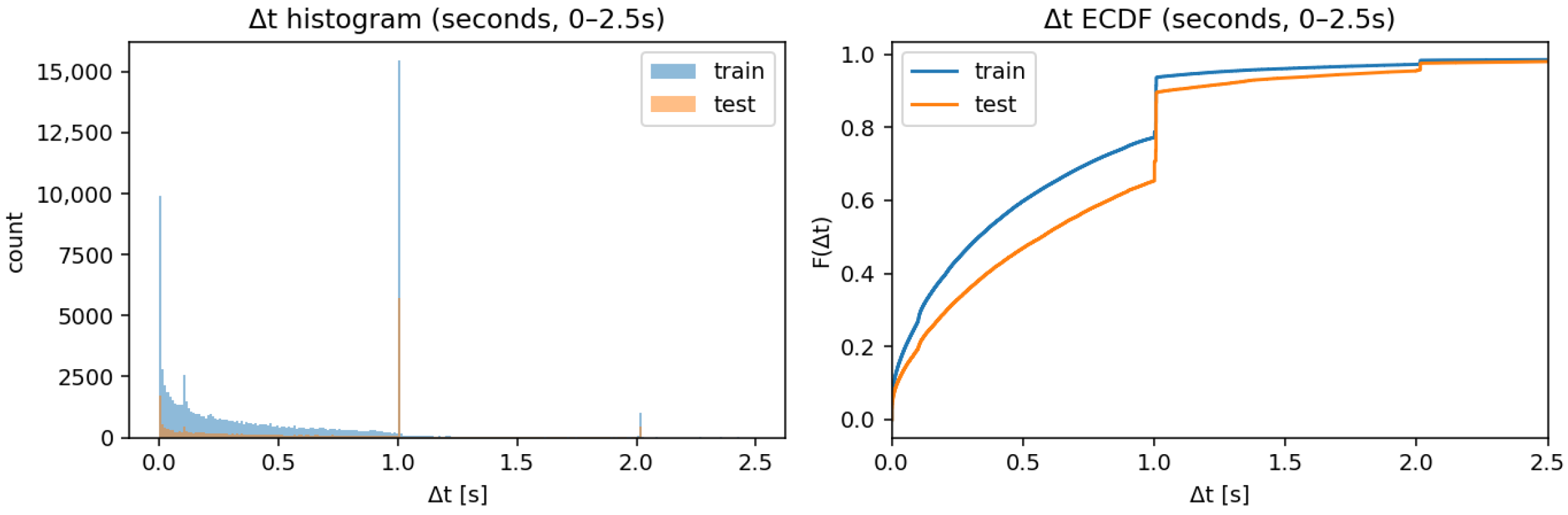
The dataset has been obtained from the Deribit exchange, which is a cryptocurrency options exchange, where at each time step, we see every available option on Bitcoin from the exchange. This effectively provides a time series of option prices, though we need to perform some pre-processing to create a static grid of strikes and maturities for the time series. This will be explored more in depth in Section 3. An important feature to note of the raw data is that it is high frequency, meaning that each consecutive snapshot is provided at the sub-second level; see Figure 1. There are 118 , 193 unique timestamps in one dataset, which spans 24 h.
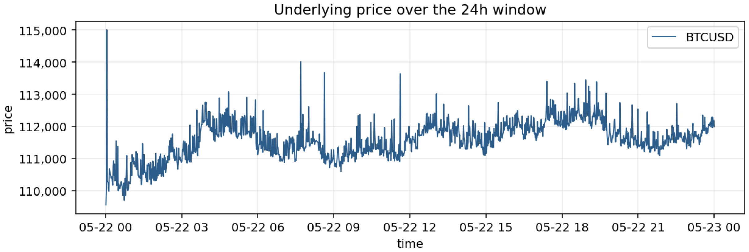
The date for the market data used in the initial experiment is 22 May 2025. For context, the price of BTCUSD on that day is plotted in Figure 2.
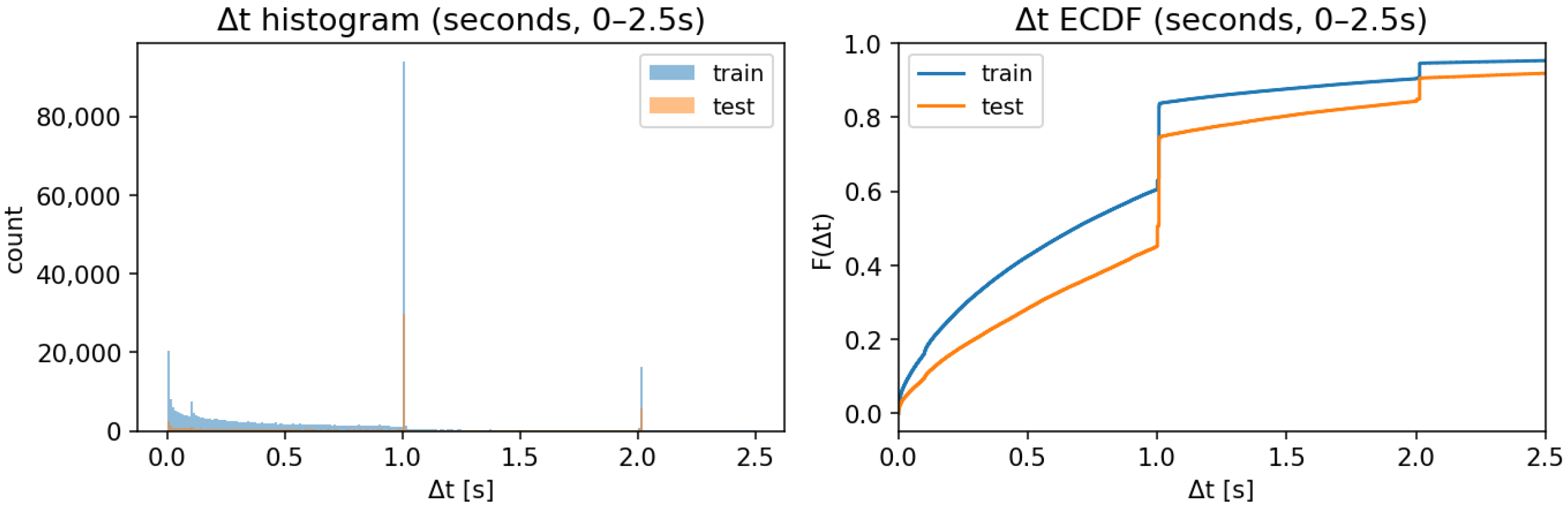
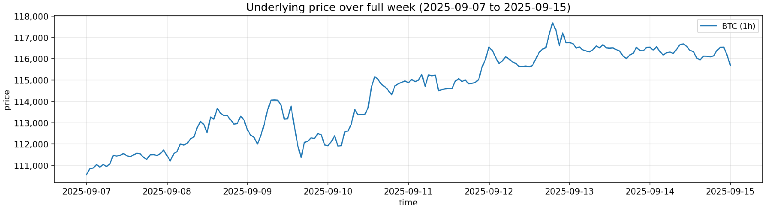
We also perform an extended analysis on a dataset following the same schema, i.e., over a week’s worth of data as opposed to a day. This extended analysis covers the dates 7–14 (inclusive) of September 2025. The distribution of time step lengths is seen in Figure 3, and the movement of the underlying asset is seen in Figure 4. This dataset has 842,940 unique time steps.
The analysis on this longer data period is conducted to complement the 24 h results of the main text and serves two purposes: to confirm that the pre-processing and decoding pipeline of Section 3 scales to a longer horizon, and to scrutinise the validity of the distributional approximations when more data are present.
The choice of data periods for which we present our empirical results, both the 24 h period for the initial analysis and the seven-day period for the extended analysis, is random and not motivated by particular market conditions. We would expect these data to be fairly representative of the market conditions prevailing in recent times.

3.2. Static Grid for Options

Over time, the time-to-maturity/moneyness coordinates of liquid options change stochastically. To facilitate training our model, it is hence required to create a static lattice of time-to-maturity/moneyness coordinates, to which market options are then matched. Let τ = T t denote time to maturity. m is forward log-moneyness, i.e.,  m = ln ( K F t ( T ) ) , with K being the strike and F t being the forward price.
It is important to note that the entire option surface is never observable at once; it is only ever a subset of options for which we currently see active quotes within the order book. Because of this, for each time to maturity τ , there is a different set of log-moneynesses m. In particular, options further from expiry have a larger range of traded moneyness values in comparison to options traded closer to maturity. This represents what Cohen et al. (2023a) call the ”liquid lattice” of options. When constructing our static grid, it is important to capture this aspect, as we are interested in modelling the movement of tradeable options that have sufficient liquidity. Conversely, we are not interested in modelling a very deep out-of-the-money option that has a one-day expiry, because we are very unlikely, given most market conditions, to observe this option ever being actively traded.

Constructinga Static Grid at High Frequency

Prior “market model” work in the literature has also parameterised the price of options in this fashion. Wissel (2008) constructs a square lattice (i.e., each maturity has the same distribution of moneyness), while Cohen et al. (2023a) use end-of-day closing data for STOXX 50 index and DAX options, which naturally provide a distribution of moneyness for each maturity, and hence the shape of the liquid lattice is chosen heuristically.
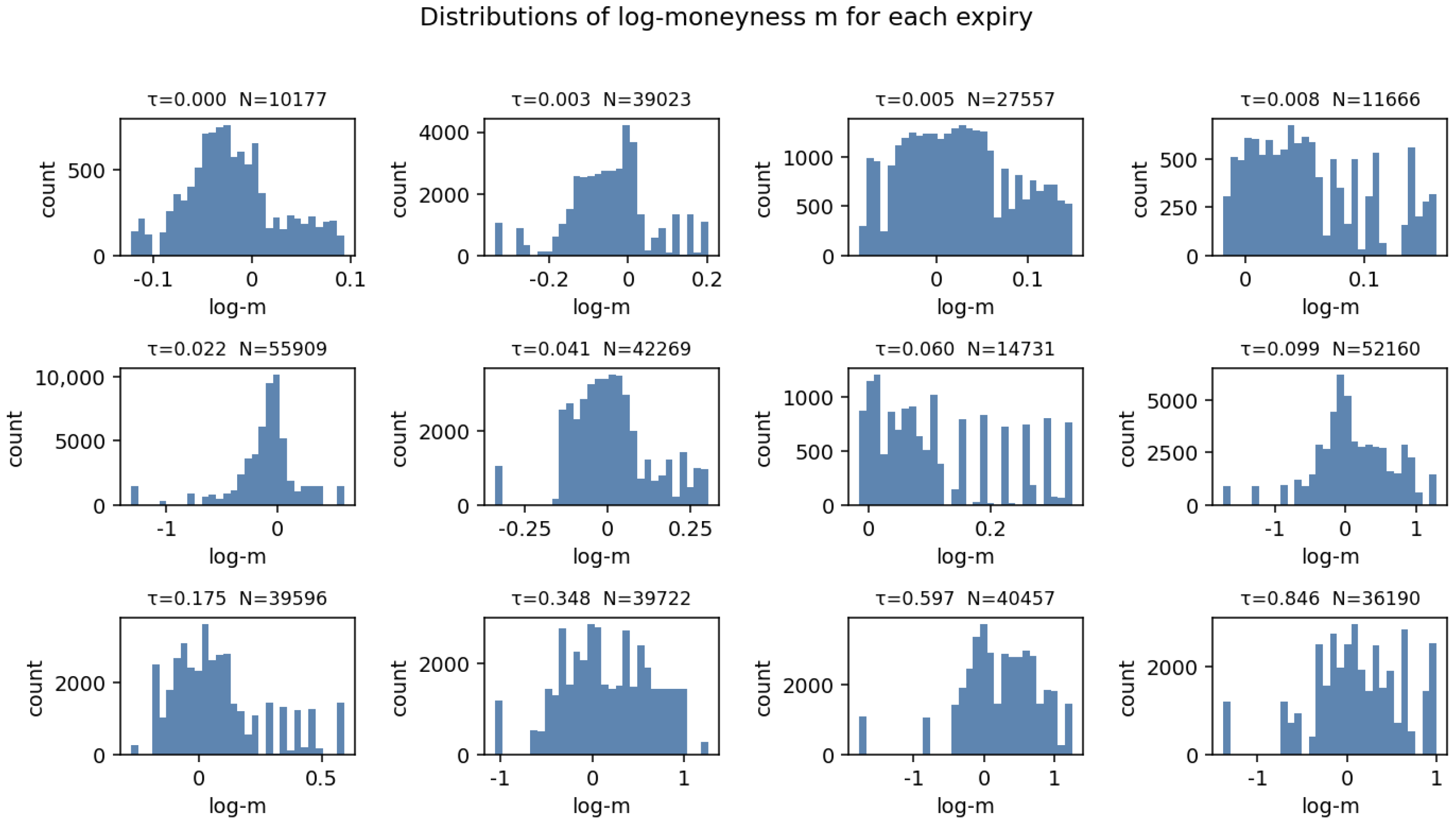
However, at high frequency/intraday frequency, each maturity has a continuous distribution of traded moneynesses effectively. Figure 5 highlights the observed distribution of available log-moneyness values for each maturity cluster in the Deribit data for a 24 h period on 22 May 2025.
This leads to a method that captures the distribution of m for each τ , or the shape of the “liquid lattice”. We are primarily interested in ensuring that this liquid lattice reflects the liquidity profile within our observed dataset. We construct a lattice over the joint ( τ , m ) space as follows. First, let { τ ¯ i } i = 1 p be the sorted unique maturities observed in the dataset. For each τ ¯ i , compute empirical moneyness percentiles m lo , i = P 1 ( m τ = τ ¯ i ) and m hi , i = P 99 ( m τ = τ ¯ i ) , and form an N m -point linear grid
m i j = m lo , i + ( j 1 ) m hi , i m lo , i N m 1 , j = 1 , , N m .
The lattice nodes are the Cartesian set N = { ( τ ¯ i , m i j ) } . We then fit a one-nearest-neighbor map in the 2D space (Euclidean metric) and assign each quote k with features ( τ k , m k ) directly to its nearest node index k = arg min ( τ ¯ i , m i j ) N ( τ k , m k ) ( τ ¯ i , m i j ) . For each calendar time t and node in N , if multiple quotes map to the same node, we keep the one with the highest liquidity (measured by trading volume). Finally, we pivot to a time-by-node panel and fill any missing entries by linear interpolation over t, followed by forward/backward-fill as needed.
This method is implemented by Algorithm 1, noting that within the 24 h of data, we take all unique maturities rather than performing clustering on τ . Let Q = { q k } k = 1 M be quote observations, where each
q k = ( t k , T k , K k , B k , A k , S k , V k , type k ) ,
with timestamp t k , expiry T k , strike K k , best bid B k , best ask A k , underlying spot S k , liquidity proxy V k (USD traded volume), and the option type. Fix reference date t ref , rates ( r , q ) , and lattice hyperparameters n τ N , n m N , and  K max N (default 50).
For each retained quote k, define
τ k : = T k t ref 365.25 , F k : = S k e ( r q ) τ k , m k : = log K k F k ,
mid k : = B k + A k 2 , c k : = mid k e ( r q ) τ k ( = C k / F k ) .
Retain calls only ( type k = C ) with V k > 0 .
If train/test splitting is used, build ( L , NN ) on the training quotes only, apply the snapping-and-panel step separately to train and test, then keep the intersection of node indices:
L = L sub train L sub test ,
and reindex both panels to L with the same linear + forward/backward fill.
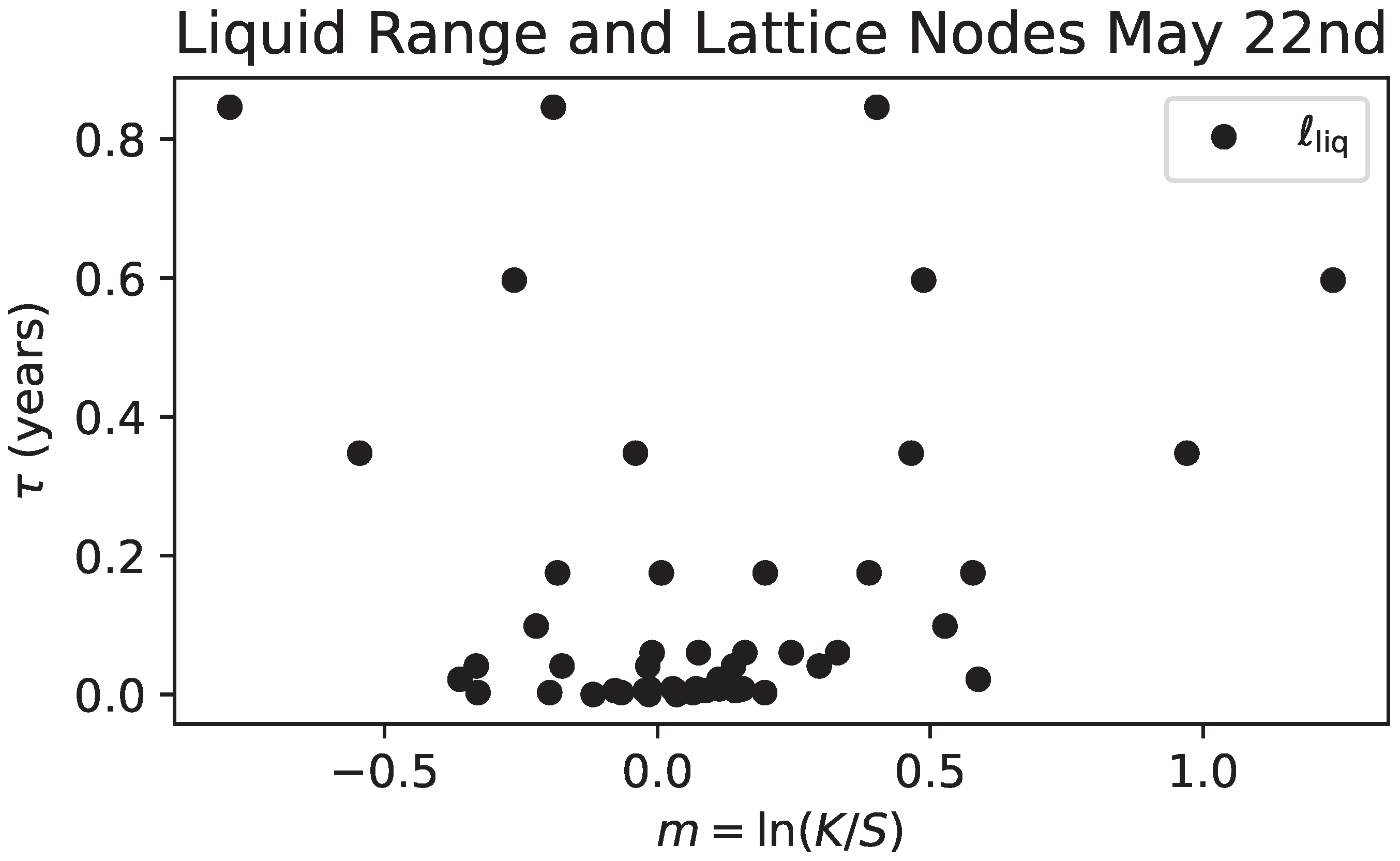
The resulting liquid lattice from this process is displayed in Figure 6, which is the lattice from 24 h of data from the 22nd of May 2025. Here we can see that, while the lattice is irregular and asymmetric, it does contain the general shape of an options lattice we would expect, with options closer to maturity having a smaller distribution support of traded moneyness values. Additionally, one can speculate that when running this process over a longer time period, say one month, the lattice would look more symmetric, as one would observe in more traded combinations of ( τ , m ) .
Algorithm 1 Static lattice construction
Require: 
Cleaned quotes { ( t k , τ k , m k , c k , V k ) } k = 1 M , n τ , n m , K max , fill method (linear)
Ensure: 
Reduced node set L sub , dense panel C ( t , ) on L sub
  1:
U sort unique { τ k } k = 1 M
  2:
Fit 1D K-means with n τ clusters on U ; obtain centroids { τ ˜ i } i = 1 n τ
  3:
Sort centroids increasingly: τ ¯ 1 < < τ ¯ n τ and relabel quote cluster indices accordingly
  4:
for  i = 1 , , n τ  do
  5:
     M i { m k : quote k assigned to cluster i }
  6:
    if  M i =  then
  7:
         ( m ̲ i , m ¯ i ) P 1 ( { m k } ) , P 99 ( { m k } )
  8:
    else
  9:
         ( m ̲ i , m ¯ i ) P 1 ( M i ) , P 99 ( M i )
10:
    end if
11:
    for  j = 1 , , n m  do
12:
         m i j m ̲ i + j 1 n m 1 ( m ¯ i m ̲ i )
13:
        Create node = ( i , j ) with coordinates x : = ( τ ¯ i , m i j )
14:
    end for
15:
end for
16:
L { x } , N : = | L | = n τ n m
17:
Fit 1-nearest-neighbor model on L in R 2 (Euclidean distance)
18:
for  k = 1 , , M  do
19:
     k arg min { 1 , , N } ( τ k , m k ) x 2
20:
end for
21:
for each pair ( t , ) observed among { ( t k , k ) }  do
22:
     I t , { k : t k = t , k = }
23:
     k ( t , ) arg max k I t , V k
24:
     C sparse ( t , ) c k ( t , )
25:
end for
26:
Set all unfilled entries of C sparse to NaN
27:
Node coverage count: n # { t : C sparse ( t , ) is observed }
28:
Keep L K = indices of the K max largest n
29:
Restrict C sparse to columns in L K ; drop columns entirely NaN
30:
Let remaining column indices be L sub and corresponding nodes be { x } L sub
31:
for each L sub  do
32:
    Interpolate C sparse ( · , ) linearly in time
33:
    Apply forward-fill, then backward-fill at time boundaries
34:
end for
35:
Denote resulting dense panel by C ( t , )
36:
return  L sub , C ( t , )

3.3. Arbitrage Repair of Historical Option Prices

When training an options model, we want to ensure that the input data is arbitrage-free. Thus cleaning input data of arbitrage violations is a logical next step in the data processing. We may encounter seeming arbitrage violations in the input data for two reasons:
  • Using the mid-price to construct our model. Within our data, and in the microstructure of markets, we do not see a single price for any asset, but rather two quotes: the bid, which is the highest price a buyer is willing to pay, and the ask, which is the lowest price a seller is willing to accept. The information contained within the spread of these relates to the liquidity of the option’s price and is captured within the lattice creation, via volume weighting, and the arbitrage-cleaning process. The existence of an arbitrage-free surface between the spread is discussed in Appendix A.
  • Data artefacts of our lattice creation method. The lattice of ( τ , m ) pairs that are created using Algorithm 1 are not guaranteed to satisfy our static-arbitrage constraints. Even if the mid-price captured a static-arbitrage-free surface, we have interpolated these prices to common nodes, which could potentially break convexity and/or monotonicity conditions.
Thus it is important to note that what may seem like arbitrage violations in the data are unlikely to be opportunities to make actual arbitrage profits in the market.
From Algorithm 1, we have a time series of option surfaces. We can use methods from Cohen et al. (2020) to “repair” these constructed surfaces of static-arbitrage violations. Note that Cohen et al. (2020) applied this method to end-of-day closing data, while in our context, it is applied to intraday, high-frequency cryptocurrency options data.
Recall the representation of static-arbitrage constraints reproduced from Cohen et al. (2020) in Section 2.2 above:
A c 0 ,
where A represents a matrix encoding each of the option shape constraints, and c is a stacked vector of call option prices, across moneyness/time-to-maturity pairs. Let A R m × N and b R m encode the shape constraints (following Cohen et al. 2020):
(i)
Monotone in maturity:
c ( τ i + 1 , m ) c ( τ i , m ) 0 .
(ii)
Monotone in strike:
c ( τ , m j ) c ( τ , m j + 1 ) 0 .
(iii)
Convex in strike:
c ( τ , m j ) c ( τ , m j 1 ) x j x j 1 c ( τ , m j + 1 ) c ( τ , m j ) x j + 1 x j , x j : = e m j .
(iv)
Bounds and intrinsic:
Lower envelope : 0 c ( τ , m ) 1 , c ( τ , m ) 1 e m + .
On a non-uniform x = e m grid, (3) is implemented as a linear inequality
1 x j x j 1 c j 1 1 x j x j 1 + 1 x j + 1 x j c j + 1 x j + 1 x j c j + 1 0 .
When adjacent τ rows have misaligned m grids, (1) evaluates c ( τ i + 1 , m ) by linear interpolation on the τ i + 1 row.
To speed up repeated projections, redundant rows of A c b are eliminated by LP tests, a method which comes from Caron et al. (1989). For each row i, solve
max c A i c s . t . A i c b i ,
where A i and b b refer to the matrix A with its ith row removed and the vector b with its ith element removed. We are trying to test if the ith constraint is redundant, so if the optimum b i + tol , row i is redundant and removed.
Subsequently, each time slice is repaired by the nearest feasible point
c ^ t = arg min c R N 1 2 c c t raw 2 2 s . t . A c b , 0 c 1 .
This strictly enforces all static constraints while minimally perturbing the raw panel. When bid/ask data is available, we perform a spread-aware L1 projection, biasing adjustments to remain within the spread by introducing non-negative up/down slack ϵ + , ϵ and weights w + , w proportional to inverse half-spreads:
min c , ϵ ± 0 n = 1 N w n + ϵ n + + w n ϵ n ,
s . t . c = c t mid + ϵ + ϵ , A c b , 0 c 1 ,
w n + = 1 max { c t , n ask c t , n mid , δ } , w n = 1 max { c t , n mid c t , n bid , δ } .
The spread-aware L1 adjustment matches the method of Cohen et al. (2020) exactly.
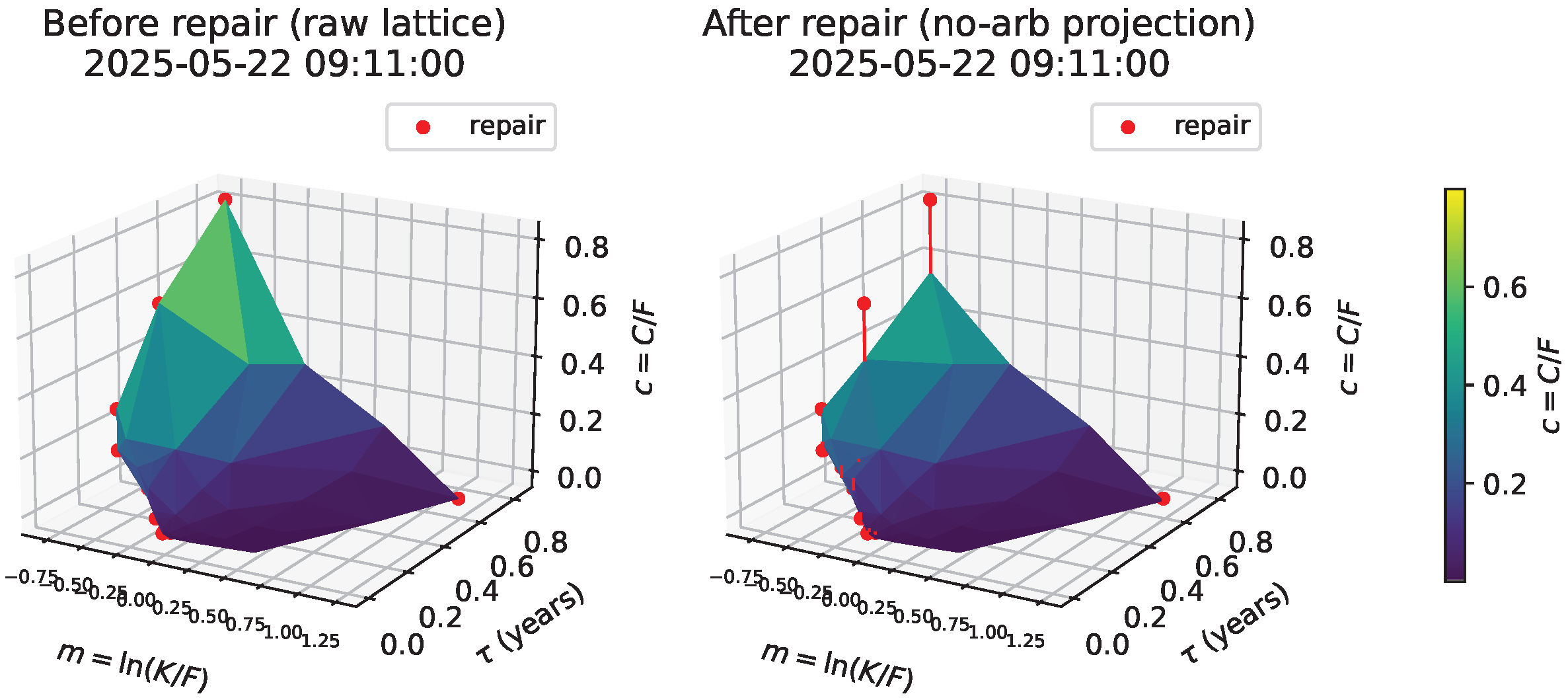
After these steps, the repaired surfaces { c ^ t } t are static-arbitrage-free and feed all downstream steps. Because each time slice solves a convex program with warm starts, the method scales to high-frequency data while remaining faithful to the observed bid–ask data. Figure 7 highlights an example of the adjustments made to create an arbitrage-free surface. We can see that the deep out-of-the-money options are the ones that have the largest corrections. This can make sense, as these options are typically the ones with the largest bid–ask spread and are also the ones with the most unreliable (and potentially stale) quotes.

3.4. Linear Factor Representation

Now that we have a series of arbitrage-free option surfaces, we notice that it is high-dimensional and that there are likely redundancies in information contained within the high-dimensional representation, in the sense that we can expect prices on the surface to be correlated in some way. As such it is useful and efficient to decompose the surface into a low-dimensional representation.
We follow the method presented in Cohen et al. (2023a), where it is labelled Algorithm 1. This algorithm is designed to decompose the surface into latent factors that are designed to minimise arbitrage in the reconstruction.
Suppose that the surface can be described by d latent factors ξ 1 t , , ξ d t , collected into the factor vector Ξ t = ( ξ 1 t , , ξ d t ) R d . We link these factors to the vector of call option prices via a linear decomposition:
c ˜ = G 0 ( τ , m ) + i = 1 d G i ( τ , m ) ξ i t .
Here G 0 ( τ , m ) R N is a baseline price vector (the temporal mean of the arbitrage-repaired surfaces) and each G i ( τ , m ) R N , i = 1 , , d , is a vector of linear loading coefficients indexed over the N lattice nodes ( τ , m ) , mapping the scalar factor ξ i t to price perturbations across the surface. Stacking the loading vectors column-wise gives the N × d loading matrix M = [ G 1 G 2 G d ] , so that (9) can be written compactly as c ˜ = G 0 + M Ξ t .
The loading vectors G i and associated factor scores ξ i t are obtained via a modified principal component analysis (PCA) procedure, following Algorithm 1 of Cohen et al. (2023a). The decomposition is performed sequentially, with each successive factor chosen to optimise a different objective:
  • Minimal Dynamic Arbitrage: The first loading vector G 1 (denoted G dyn ) is chosen to align with the leading principal component of the empirical z-factor, i.e., the deterministic drift operator applied to the reconstructed surface (see Appendix B). This ensures the dominant direction of surface evolution is representable by the factor model, thereby minimising the violation of the HJM-type drift restriction. It is worth noting that this approach to minimising dynamic arbitrage in the model is by the construction of an approximation, justified by the fact that dynamic arbitrage opportunities are only practicable if they are relatively large (given that truly continuous-time trading is not possible and any such arbitrage strategies would be subject to substantial model risk).
  • Statistical Accuracy: The second loading vector G 2 (denoted G stat ) is the leading principal component of the residual price variation after projecting out G 1 . This captures the direction of the maximum remaining variance, ensuring accurate reconstruction.
  • Minimal Static Arbitrage: The third loading vector G 3 (denoted G sa ) is chosen from the residual subspace to minimise the static-arbitrage violations (measured via the constraint matrix A) in the reconstructed surfaces. A hinge-penalty objective penalises violations of A c ˜ 0 during the optimisation of this direction.
The loading matrix is therefore partitioned as M = [ G dyn G stat G sa ] under a three-factor model ( d = 3 ).
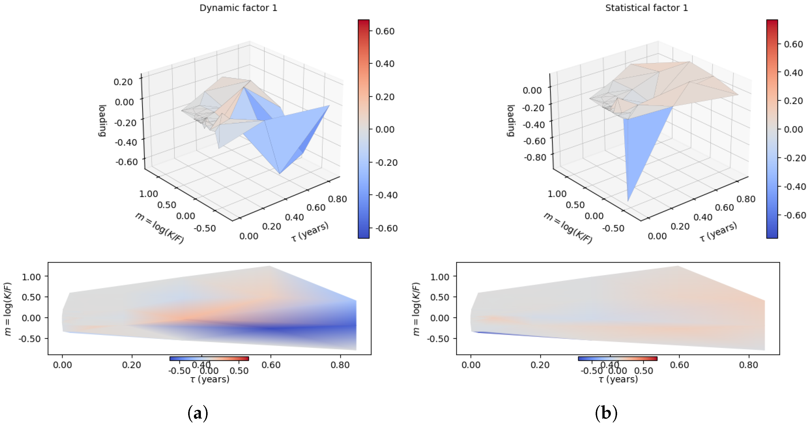
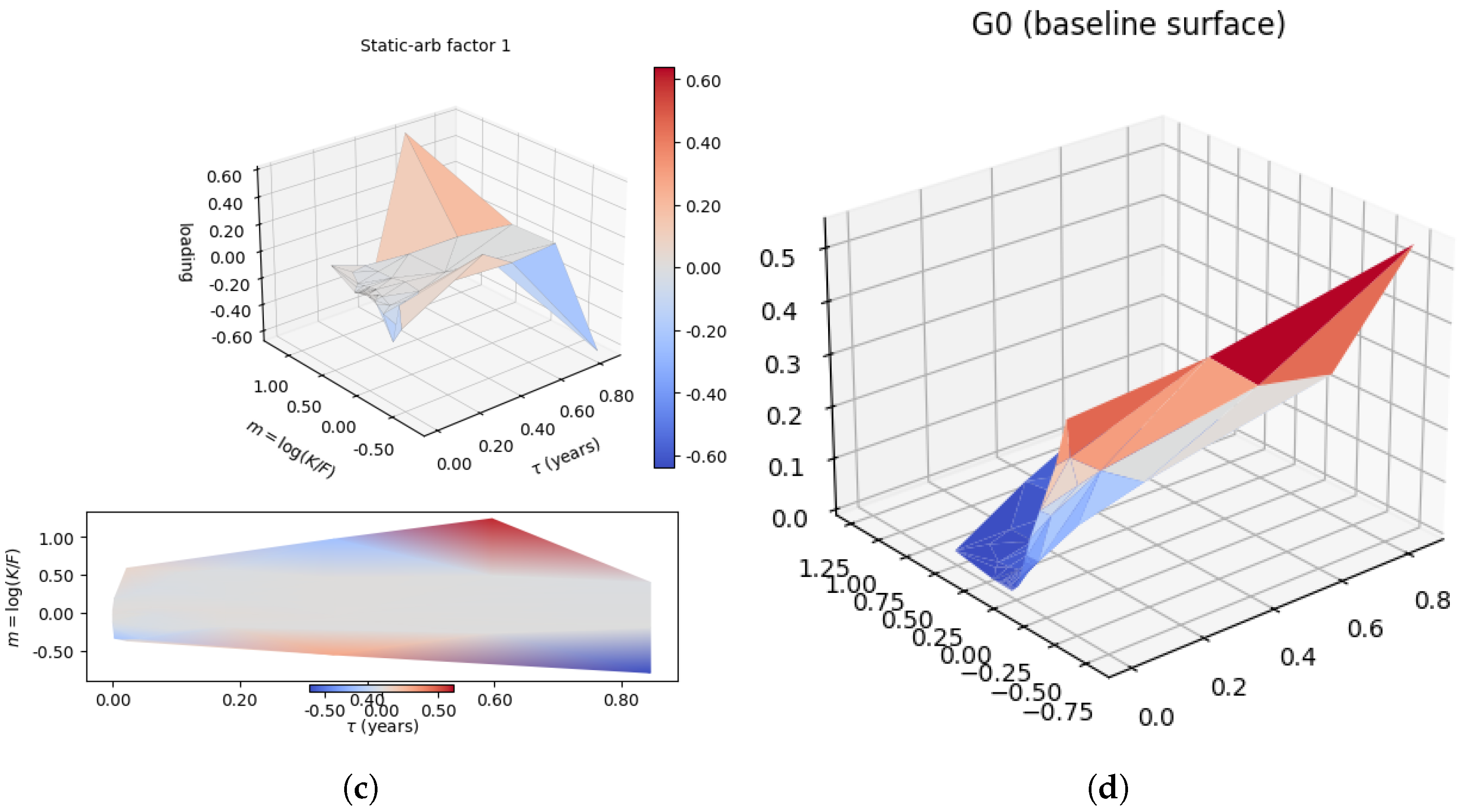
Figure 8 illustrates the three loading vectors and the baseline G 0 under a three-factor model. While the stochastic loading vectors are difficult to interpret individually, the baseline G 0 exhibits the standard call surface shape one would expect. Similar to the approach by Cohen et al. (2023a), all loading vectors G i ( i 1 ) are hard-coded to zero at maturity τ = 0 to ensure that the terminal payoff condition is satisfied.

4. Neural SDE Modelling

This section builds on the method of Cohen et al. (2023a), applying it to high-frequency cryptocurrency options data to obtain a data-driven, arbitrage-free model taking in the time series of available cryptocurrency option market data.

4.1. Stochastic Dynamics of Market Factors

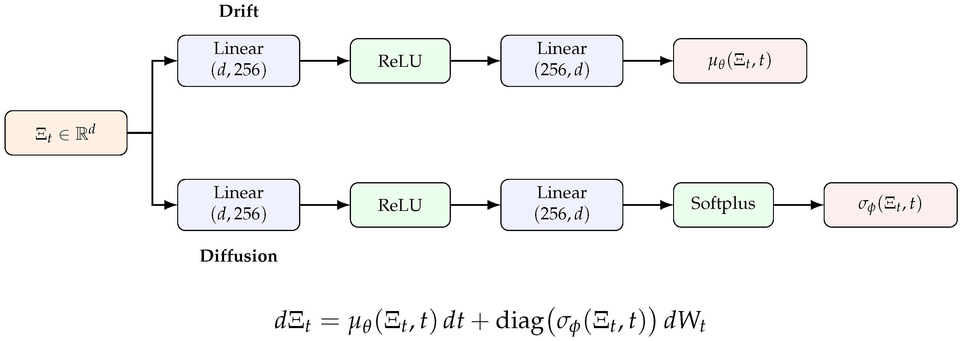
We first posit an SDE for the evolution of our market factors under the statistical (a.k.a. “objective”, “physical” or “real-world”) probability measure, commonly denoted as the P measure. Specifically, the dynamics of the d-dimensional factor vector Ξ t = ( ξ 1 t , , ξ d t ) introduced in Section 3.4 are assumed to be governed by the SDE,
d Ξ t = μ θ ( Ξ t , t ) d t + σ ϕ ( Ξ t , t ) d W t ,
where μ θ is the drift vector, σ ϕ is the diagonal diffusion matrix and W t is a standard Brownian motion. Each of μ θ , σ ϕ and W t is d-dimensional, where d refers to the number of factors chosen from our factor decoding, as described in Section 3.4. Our diffusion matrix is assumed to be diagonal, meaning we assume that the noise terms between our Ξ factors are uncorrelated, and with the 24 h of data, this assumption seems to hold relatively well when analysing the residual factor plots; see Section 4.4.2.
In our data-driven approach, we represent the drift and diffusion components of this SDE with neural networks with weights θ and ϕ respectively. The specific architecture of the neural networks is detailed in Appendix E.
We can formulate the loss function for training the neural networks in this model by considering the Euler–Maruyama discretisation for a stochastic differential equation. Under this expansion, we have a defined transition. Let Δ t k : = t k + 1 t k and Δ W k : = W t k + 1 W t k N ( 0 , Δ t k I d ) . The Euler–Maruyama step for the Itô SDE is
Ξ k + 1 = Ξ k + μ θ ( Ξ k , t k ) Δ t k + σ ϕ ( Ξ k , t k ) Δ W k , = Ξ k + μ θ ( Ξ k , t k ) Δ t k + σ ϕ ( Ξ k , t k ) Δ t k ε k , ε k N ( 0 , I d ) .
Conditionally on Ξ k , the transition density is Gaussian:
Ξ k + 1 Ξ k N m k , Δ t k Γ k , m k : = Ξ k + μ θ ( Ξ k , t k ) Δ t k , Γ k : = σ ϕ ( Ξ k , t k ) σ ϕ ( Ξ k , t k ) .
We can then formulate an expectation maximisation (EM) loss function. Define the observed increment Δ Ξ k : = Ξ k + 1 Ξ k . The one-step negative log-likelihood (NLL) is
k ( θ , ϕ ) = 1 2 [ Δ Ξ k μ θ ( Ξ k , t k ) Δ t k Δ t k Γ k 1 Δ Ξ k μ θ ( Ξ k , t k ) Δ t k + log det Δ t k Γ k + d log ( 2 π ) ] ,
so that for a path { Ξ k } k = 0 K , the total loss function value is
L NLL ( θ , ϕ ) = k = 0 K 1 k ( θ , ϕ ) .
This NLL function now formulates our test loss, where minimising the NLL is equivalent to maximising the likelihood of seeing the next step given the current data. This follows the classical EM framework from Dempster et al. (1977) and is the neural SDE learning strategy from Dridi et al. (2021). This is structurally analogous to the maximisation/inference loop approach from Greff et al. (2017).
This training scheme does make the assumption that the transition/discretisation of the process is Gaussian, and at ultra-high frequency (sub-second level intervals), this assumption does not hold. When using 24 h of high-frequency cryptocurrency options data, the prices were aggregated, by taking the median price, to minutely increments in order for goodness-of-fit tests to look reasonable. The training results at high frequency and the associated discussion can be found in Appendix C.
One can also consider using different expansions or quasi-likelihoods as the loss term for the SDE. Aït-Sahalia (2002) develops a closed-form approximation for the likelihood of discretely observed diffusion processes, addressing the fact that most continuous-time SDEs lack an analytically tractable transition density. The approach constructs a sequence of explicit Hermite polynomial expansions that converge uniformly to the true but unknown transition density. By successively correcting the leading Gaussian term through higher-order terms in the sampling interval Δ t , this method yields a quasi-maximum likelihood estimator that remains asymptotically equivalent to the true MLE. Conceptually, it extends the Euler–Maruyama Gaussian transition by incorporating higher-order corrections that depend on the local drift, diffusion, and their spatial derivatives, thereby capturing the non-linearity and skewness inherent in finite-time transitions. We explored using this approximation as a higher-order likelihood correction to the Gaussian transition in (12), attempting to capture the non-Gaussianity of the high-frequency intervals, and the training results in this case are presented and discussed in Appendix D.

4.2. Arbitrage-Free Factor Representation

In order to constrain the outputs of our model to be free of static arbitrage, we must first consider what these constraints mean in our factor space. As our constraints are linear inequalities and our factor representation of option prices is also linear, these constraints have a representation in the factor space. Recall the linear constraints in Section 2.2, A c 0 and the linear factor decomposition, c ˜ = G 0 ( τ , m ) + i = 1 d G i ( τ , m ) ξ i t . Substituting this decomposition into the constraint system gives
A c ˜ = A G 0 + i = 1 d A G i ξ i t 0 .
Hence, in the factor space, the arbitrage-free region is characterised by all factor vectors Ξ t = ( ξ 1 t , , ξ d t ) , satisfying
A G Ξ t b G , A G : = [ A G 1 , A G 2 , , A G d ] , b G : = A G 0 .
This defines a convex polytope, or region of space, in the factor space, within which any combination of factors yields option prices that respect all static-arbitrage constraints. During training or simulation, we therefore enforce that the decoded factors Ξ t remain inside this feasible region
P arb = Ξ t | A G Ξ t b G ,
ensuring that the reconstructed surface is statically arbitrage-free.
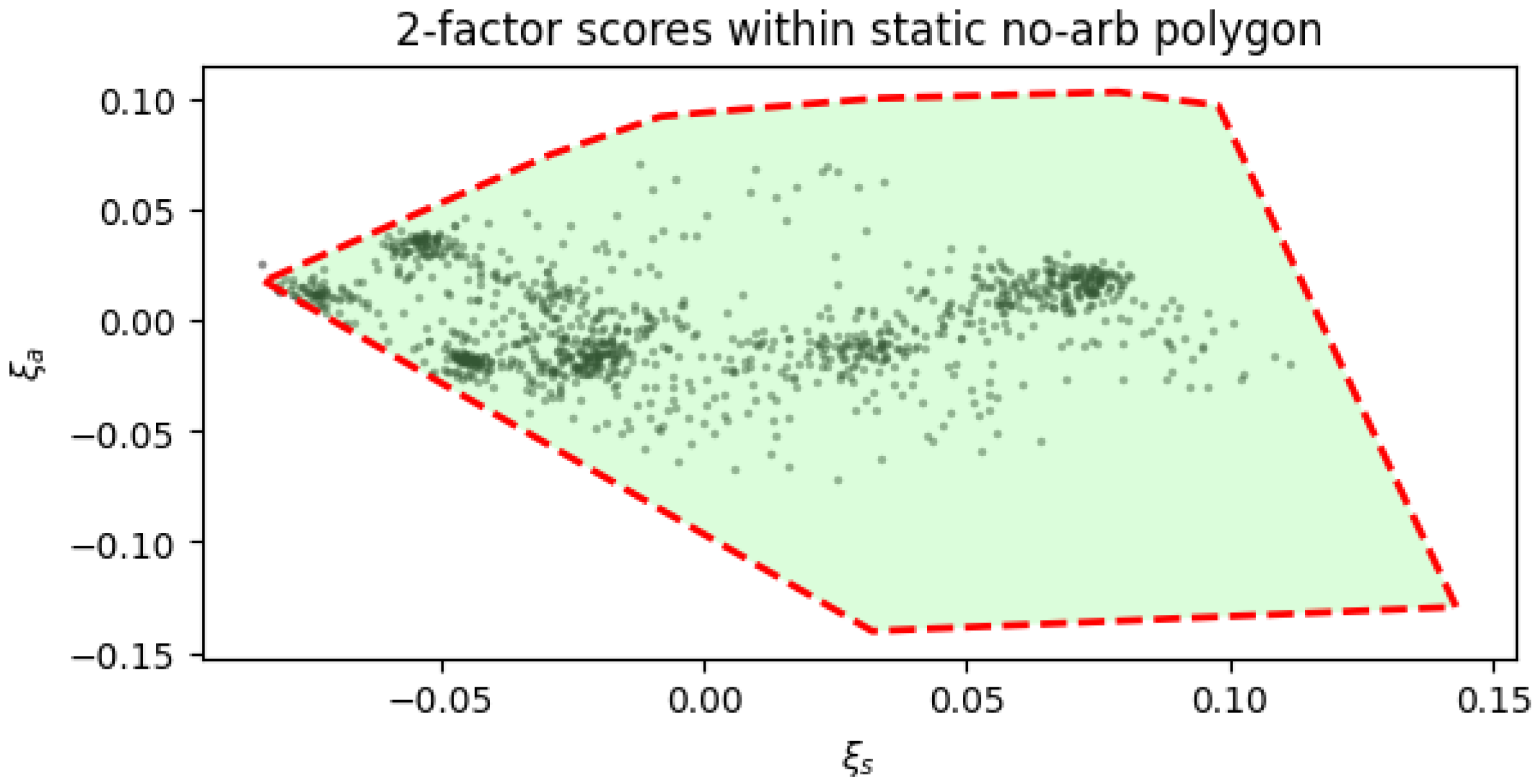
Removing redundant linear constraints, as described in Section 3.3, we can plot our static-arbitrage-free convex polytope and the associated ξ factors to visually inspect if our factor decoding process in Section 3.4 has been done correctly. Figure 9 presents scores in a two-factor model and the corresponding static no-arbitrage polygon. Inspecting this image we can see that the vast majority of our latent ξ factors lie within the acceptable polygon. Those few scores, which lie either on the boundary or just outside the polygon, are there due to the hinge-penalty-based optimisation done to reduce static arbitrage in option price reconstruction in the factor decoding process given in Section 3.4.

4.3. Constrained Networks and No-Static-Arbitrage Guarantees

Given the specified region of space in which the Ξ factors can evolve without option prices allowing static arbitrage, we can enforce constraints on the neural SDE to ensure that the process remains within the required polytope. Cohen et al. (2023a) provide the method to achieve this using Friedman and Pinsky conditions for the non-attainability of a boundary for an SDE (Friedman and Pinsky 1973).
Definition 1 
(Friedman–Pinsky non-attainability conditions). Consider an Itô diffusion in R d ,
d Ξ t = μ ( Ξ t ) d t + σ ( Ξ t ) d W t ,
and let P = { Ξ R d : a i Ξ b i , i = 1 , , n f } be a convex polytope defined by n f linear constraints (i.e., n f faces). For each face i with the boundary function
q i ( Ξ ) : = a i Ξ b i = 0 ,
define the normal drift and diffusion components near the boundary as
μ i ( Ξ ) : = a i μ ( Ξ ) , σ i 2 ( Ξ ) : = a i Γ ( Ξ ) a i , Γ ( Ξ ) : = σ ( Ξ ) σ ( Ξ ) .
Then, a sufficient condition for the boundary P to be non-attainable (i.e., the process remains in P almost surely if started inside) is that, for each i,
( i ) μ i ( Ξ ) 0 whenever q i ( Ξ ) = 0 ,
( ii ) σ i 2 ( Ξ ) = 0 whenever q i ( Ξ ) = 0 .
That is to say, the drift of the SDE points inward at the boundary, and the diffusion vanishes in the direction normal to it.
Cohen et al. (2023a) enforce these conditions via a smooth Lipschitz function. This function will shrink the diffusion as it gets closer to the boundary and slowly add drift in the opposite direction. Choosing such a function to be smooth and Lipschitz is important so as not to break backpropagation for training the neural networks. Recall the linear price map c ˜ = G 0 + M Ξ t from (9), where Ξ t R d is the factor vector and M = [ G dyn G stat G sa ] R N × d is the loading matrix. Given the lattice constraints A c ˜ b , we map them into factor space as
H Ξ t h , H : = A M , h : = b A G 0 ,
and augment with a data-driven box L Ξ t U . The box bounds L , U R d are obtained component-wise from the training factor scores as L k = Q α ( { ξ k , t } t ) and U k = Q 1 α ( { ξ k , t } t ) for a small quantile level α (defaulting to component-wise min/max when quantile trimming is not applied). These box constraints are converted into additional half-space rows appended to H Ξ t h , so that the diffusion shrinkage and inward drift correction treat empirical range boundaries identically to the static-arbitrage faces. Let n f denote the total number of half-space constraints (arbitrage faces plus box faces) after this augmentation. Rows of H are row-normalised when building the shrink geometry, so the signed distance of Ξ t to face i is
ρ i ( Ξ t ) : = H i Ξ t h i H i = H i Ξ t h i ( since H i   =   1 ) .
Following Cohen et al. (2023a) the Lipschitz shrink profile is given by
ϕ ( x ) = x + 1 + x + , x + : = max { x , 0 } .
Near the boundary ρ i ( Ξ i ) 0 , we have ϕ ( ρ i ) 0 , far inside the polytope ϕ ( ρ i ) 1 .
At a given state Ξ t we select the k = min { d , n f } most relevant faces (smallest ρ i ), build an orthonormal frame Q ( Ξ t ) R d × d whose first k columns point along the corresponding unit normals, and compute shrink coefficients ε ( Ξ t ) [ 0 , 1 ] k with components ε j ( Ξ t ) = ϕ ( ρ i j ( Ξ t ) ) . This yields two equivalent shrink operators (chosen by mode):
-
Matrix shrink:
P ( Ξ t ) = Q ( Ξ t ) diag ( ε ( Ξ t ) ) 0 0 I d k Q ( Ξ t ) R d × d ,
so the effective diffusion is
Γ eff ( Ξ t ) = P ( Ξ t ) Γ ( Ξ t ) P ( Ξ t ) .
-
Diagonal shrink (default, diagonal noise): Compute elementwise multipliers s ( Ξ t ) [ 0 , 1 ] d so that diag ( s ( Ξ t ) ) σ ( Ξ t ) best matches P ( Ξ t ) diag ( σ ( Ξ t ) ) in a covariance sense. The effective diffusion used inside the model is
σ eff ( Ξ t ) = s ( Ξ t ) σ ( Ξ t ) .
In both cases, along any active face normal a i , one has a i Γ eff ( Ξ t ) a i 0 as ρ i ( Ξ t ) 0 , satisfying (16). The same shrink can also be applied at the loss level: rather than modifying the diffusion σ directly, the constraint geometry is absorbed into a state-dependent preconditioner Ω ( Ξ t ) R d × d (derived from P ( Ξ t ) ) that transforms the observed increments and likelihood. Specifically, the tuple ( Ω , det Ω , Ω Δ Ξ ) is passed to the negative log-likelihood (13), so that the Gaussian transition is evaluated in the preconditioned coordinate system where the boundary constraints are automatically respected.
To enforce (15) via an inward drift correction, we precompute, along the observed factor path X t , per-time inward directions and normalised boundary distances using
( dirs t , ε t μ ) = ( W , b , X · ; ρ , ε μ ) ,
where ( W , b ) are the row-normalised half-spaces from the polytope output. At the training time, for a batch indexed by t, the raw drift μ ( · ) is corrected by
μ corr ( X t ) = μ ( X t ) + Δ μ t , Δ μ t = k w t , k dirs t , k , w t , k = λ bc ε t , k μ + ε 0 1 { ε t , k μ τ cut } ,
with user-selectable parameters ( λ bc , ε 0 , τ cut ) and an optional norm cap Δ μ t     cap .
Together, the smooth diffusion shrink guarantees a i Γ eff ( Ξ t ) a i 0 as the boundary is approached, and the inward drift correction ensures a i μ corr ( Ξ t ) 0 there; hence the Friedman–Pinsky non-attainability conditions are satisfied for the learned SDE on the static-arbitrage polytope.

4.4. Training Results on Single-Day Data

This section will discuss and review training results and goodness-of-fit tests of this neural SDE model on our Deribit cryptocurrency options data from 22 May 2025.

4.4.1. Loss Curve

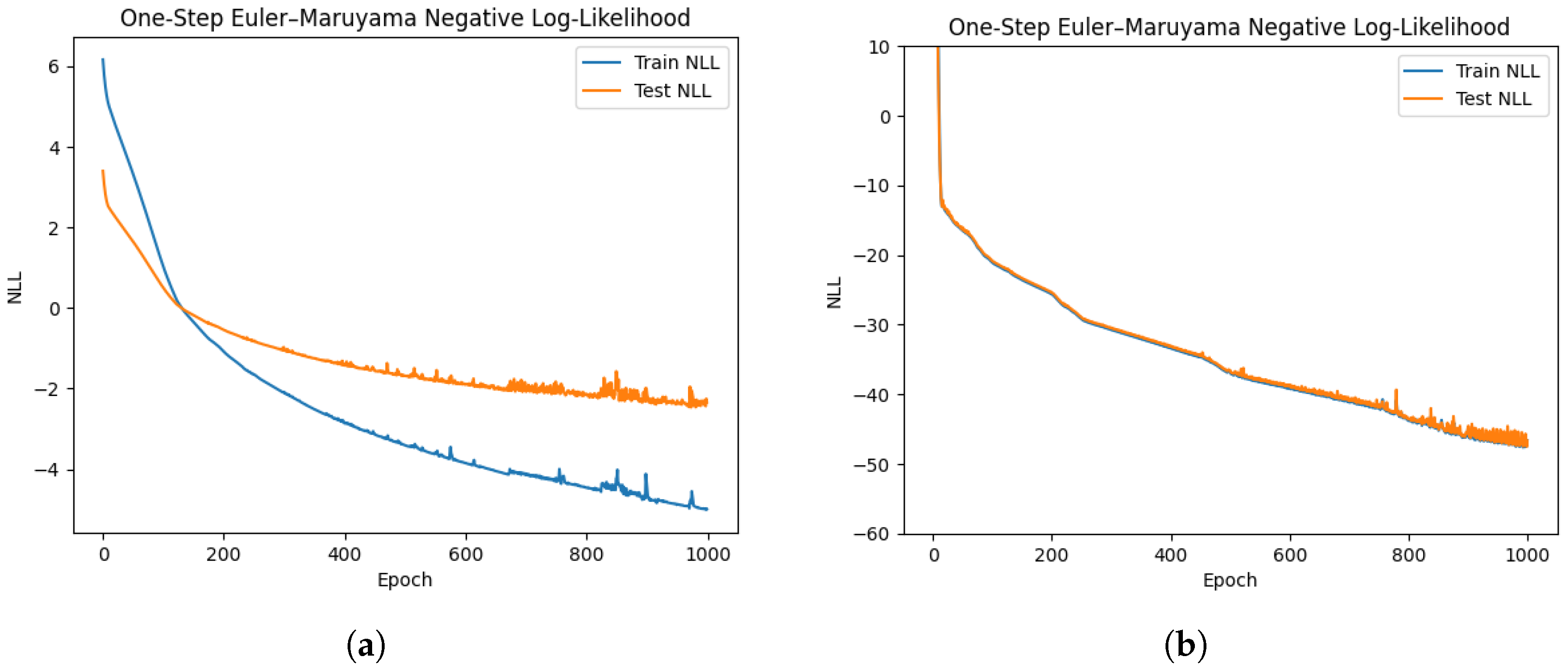
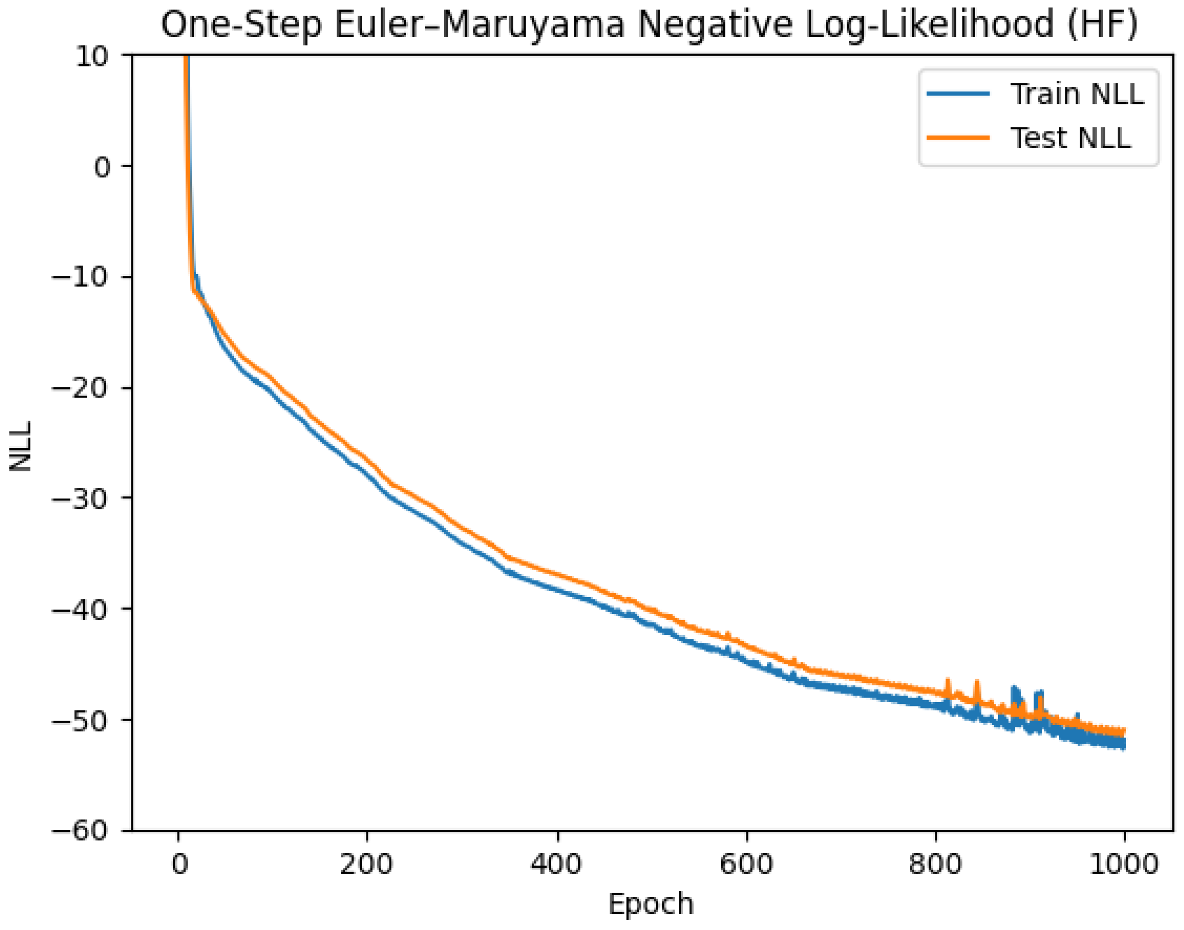
Illustrated in Figure 10, each loss curve, with and without the drift/diffusion constraints, suggests convergence. However, the loss with the constraints is far lower than the loss without them. Additionally, the gap between the train and test loss is smaller. This is interpreted as suggesting that the constraints are indeed working as expected, reducing the state space of our Ξ factor values.
Here, the train/test split is 80/20. Meaning, the first 80% of the 24 h period is used as training, and the remaining 20% is the test, or out-of-sample, region.

4.4.2. Residual Plots

Following the estimation of the neural SDE, we assess the adequacy of the fitted drift and diffusion functions by examining the one-step standardised residuals. Under the Euler–Maruyama discretisation of the stochastic differential equation
d Y t = μ θ ( Y t ) d t + σ ϕ ( Y t ) d W t ,
the discrete-time transition between observations can be approximated as
Y t + Δ t Y t + μ θ ( Y t ) Δ t + σ ϕ ( Y t ) Δ t ε t , ε t N ( 0 , I d ) ,
where ε t are the model innovations implied by the fitted dynamics. Given observed data { Y t } t = 1 T , we therefore compute the empirical residuals as
ε ^ t = Y t + Δ t Y t μ θ ( Y t ) Δ t σ ϕ ( Y t ) Δ t .
If the estimated SDE correctly captures the conditional mean and variance of the data, then ε ^ t should be approximately independent and standard normal across time and dimensions.
These residuals thus serve as a key diagnostic measure: quantile–quantile (QQ) plots of ε ^ t against a standard normal distribution test for deviations from Gaussianity (such as skewness or excess kurtosis), while pairwise scatter plots of ε ^ t ( i ) and ε ^ t ( j ) assess the cross-sectional independence across latent factors.
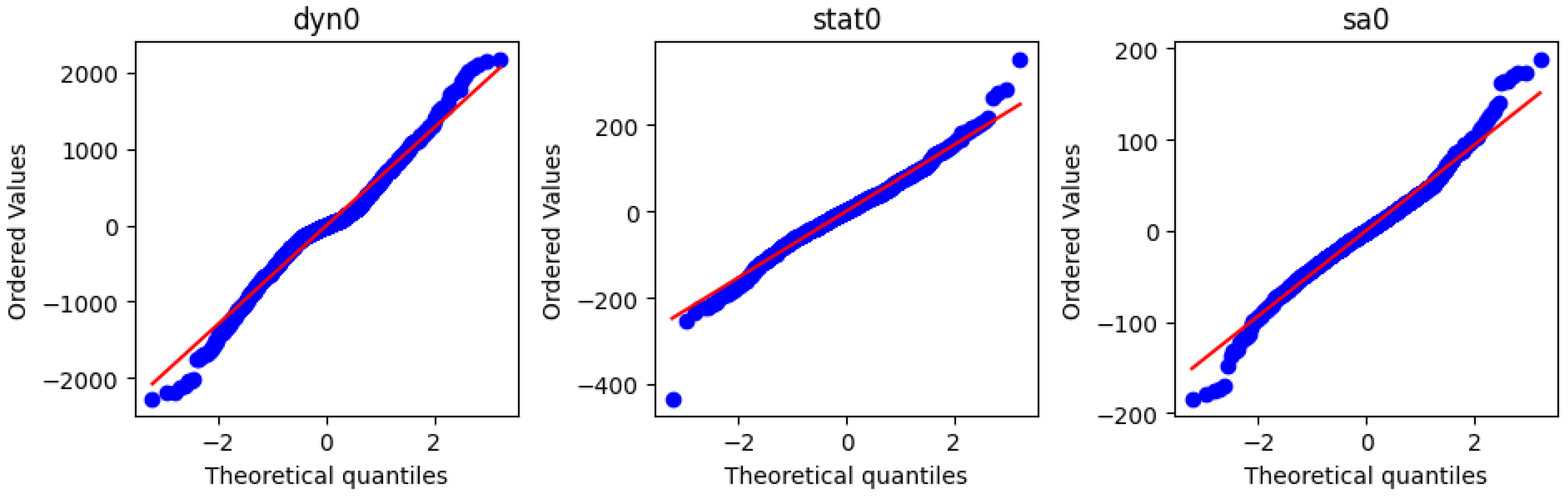
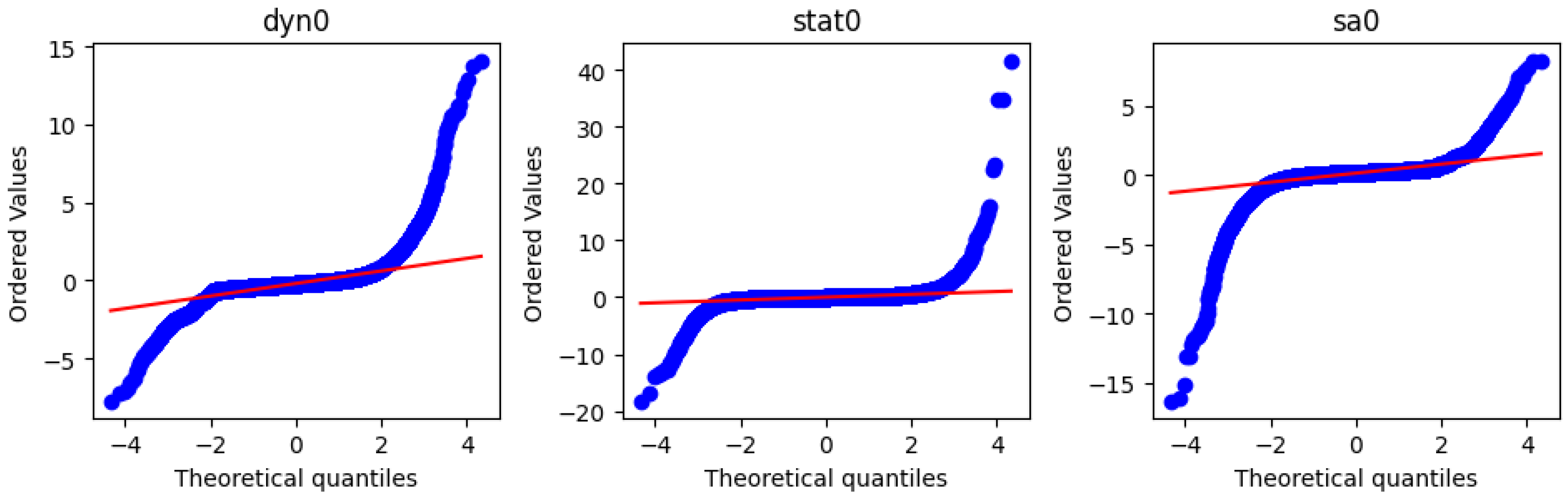
From the QQ plots in Figure 11, we can see that the assumption of Gaussian transition increments from our Euler–Maruyama training step is approximately correct, though not perfect. There is still some overdispersion at the tails and underdispersion at the centrality. This suggests that deviations from our model predictions are still possible, which makes sense considering the cryptocurrency market’s higher volatility.
In addition to marginal normality checks, we also compute the pairwise correlations between residual components to evaluate the cross-sectional independence of the model’s innovations. For each pair of factors ( i , j ) , the sample correlation coefficient is given by
ρ i j = Cov ( ε ^ ( i ) , ε ^ ( j ) ) Var ( ε ^ ( i ) ) Var ( ε ^ ( j ) ) .
Under a correctly specified diffusion, the residuals should be uncorrelated across factors, reflecting that each dimension of the learned SDE captures an independent source of risk or market variation.
Analysing the residuals as plotted in Figure 12, we can see that there is some slight correlation between the “dynamic arbitrage” factor and the “statistical accuracy” factor. In a sense, this is not unexpected, as in testing, we noticed that the vast majority of variance is explained with a two-factor model. When training with two factors (one statistical-accuracy factor and one static-arbitrage factor), we observe an R 2 value of 99.5–99.8%, indicating that almost all variation in the observed option prices is captured by the model’s reconstructed surfaces. In this context, R 2 measures the proportion of the total price variance explained by the factor representation, reflecting both the completeness and goodness-of-fit of the decomposition. In a way this is unsurprising, as other martingale stochastic volatility models are also two-factor models (see, e.g., Hagan et al. 2002; Heston 1993). Aside from that, the correlations are low, and the residuals are centre-aligned.

4.5. Training Results of a Week of Data

This section reports the calibration of the arbitrage-free neural SDE on the extended dataset introduced in Section 3.1, comprising the trading week of 7–14 September 2025, whose timestamp-spacing and underlying-price profiles are shown in Figure 3 and Figure 4. It complements the 24 h results above and serves two purposes: to confirm that the pre-processing and decoding pipeline of Section 3 scales to a longer horizon, and to scrutinise the distributional assumptions underlying the Gaussian likelihood and the diagonal diffusion when more data, spanning more market regimes, are present.

4.5.1. Liquid Lattice for the Week

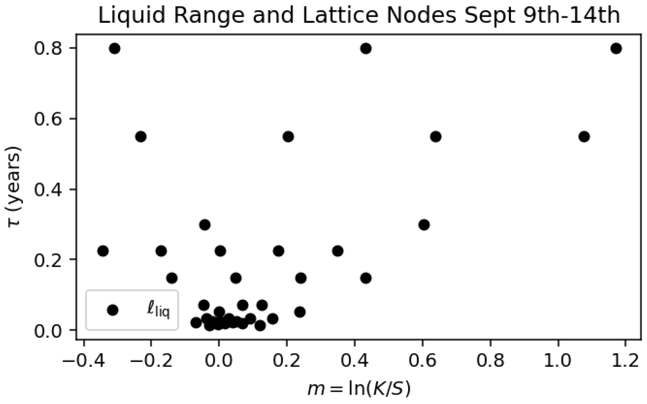
Figure 13 shows the liquid lattice N obtained for the week through the construction of Section 3.2. It exhibits the characteristic shape of an options lattice: a dense concentration of nodes at short maturities ( τ < 0.1 ) and near the money, with the traded moneyness range widening at longer maturities, where nodes extend from roughly m = 0.35 to m = 1.2 . The maturities cluster into a small number of discrete buckets ( τ 0.02 0.08 , 0.15 , 0.22 , 0.30 , 0.55 , 0.80 years), reflecting the maturity-clustering step of Algorithm 1, and the lattice contains 39 nodes in total. Relative to the single-day lattice of the main text, the week’s lattice is denser and spans a wider moneyness range, because more ( τ , m ) combinations become liquid once aggregated over five trading days; as shown in Appendix F.3, this is precisely the regime in which the factor representation is best identified.
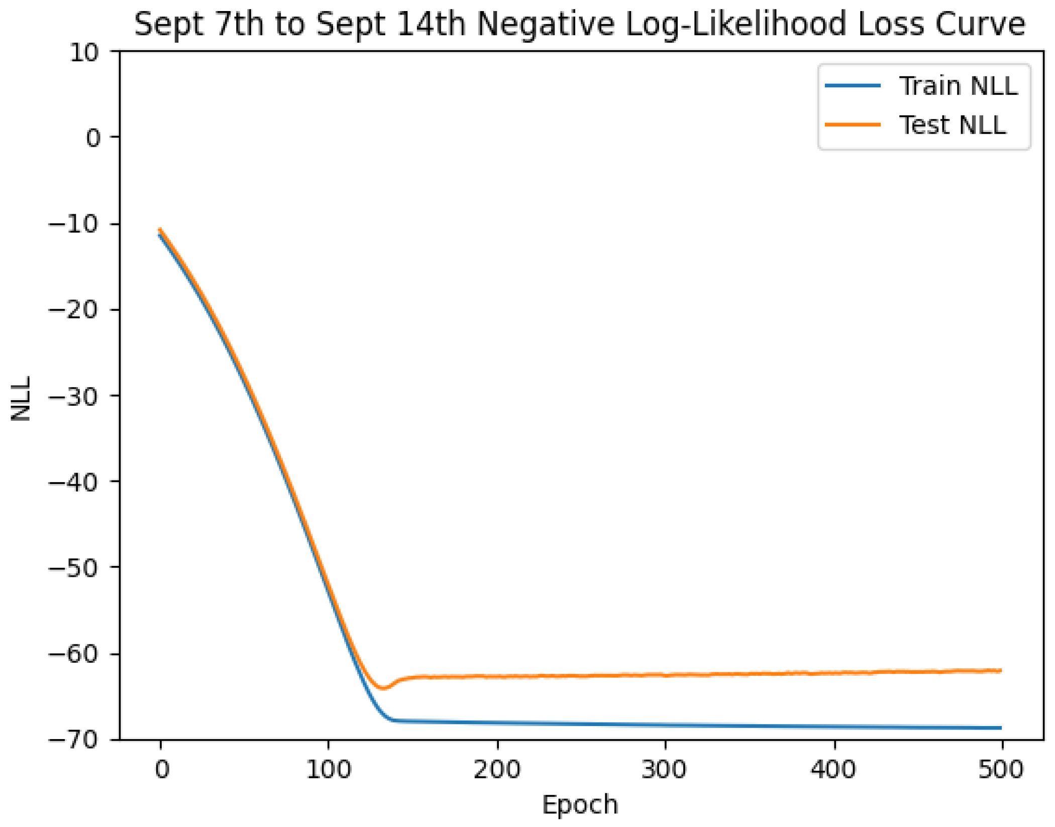
As Figure 14 shows, on this data set the training and test negative log-likelihood is also well-behaved: The objective function converges within ≈130 epochs and then flattens out, leaving a small and stable train/test gap with no deterioration of the test loss.

4.5.2. Residual Diagnostics: Marginal Normality

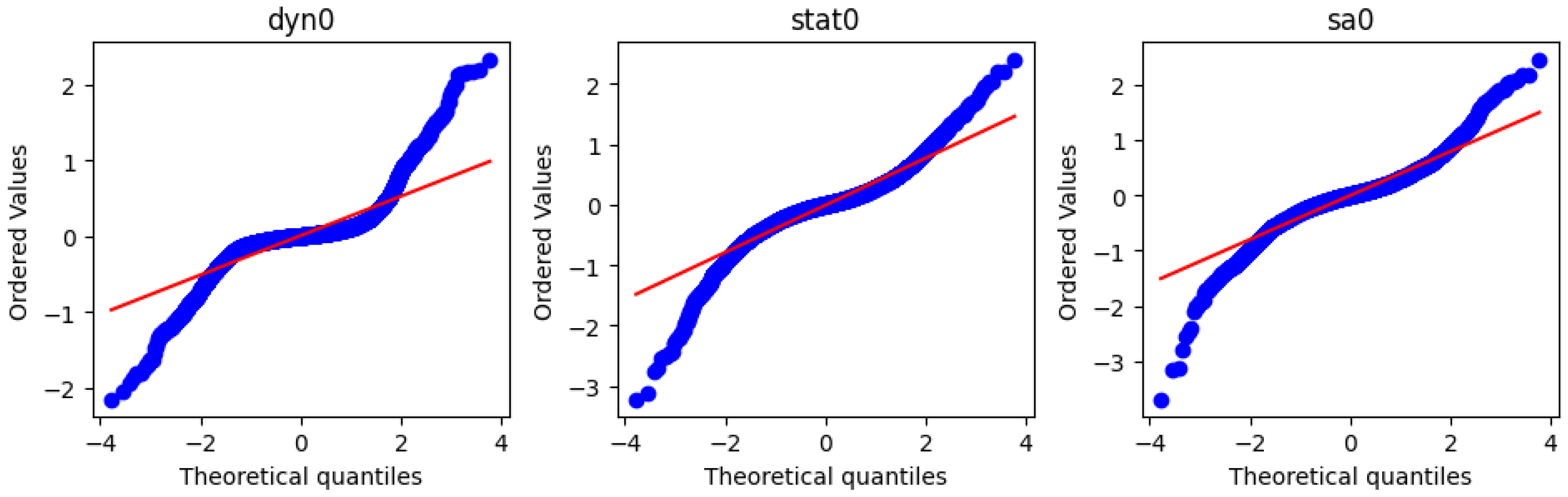
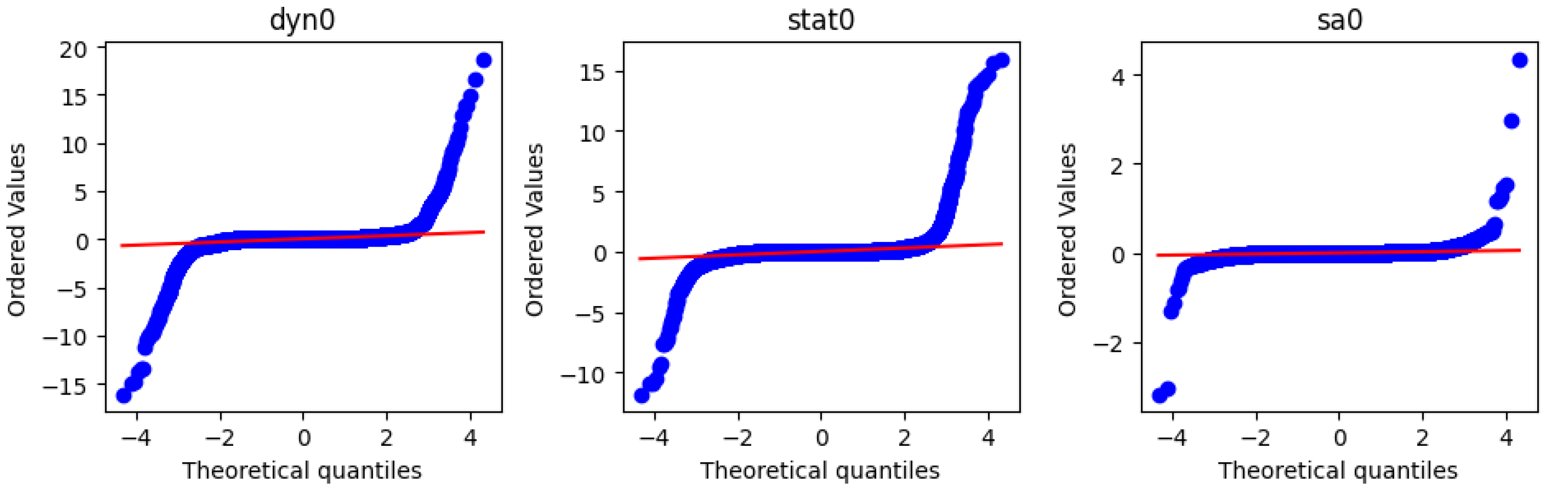
The likelihood treats each one-step factor increment as conditionally Gaussian. To assess this, Figure 15 presents normal quantile–quantile plots of the standardised one-step residuals of the three factors ( G dyn , G stat and G sa ).
We can see that while all three are still approximately linear, there are fatter tails in the QQ plot in comparison to when training over only a single day. The dynamic factor is the most peaked, with its near-flat central segment indicating a concentration of small increments punctuated by occasional large moves.

4.5.3. Residual Diagnostics: Cross-Factor Dependence

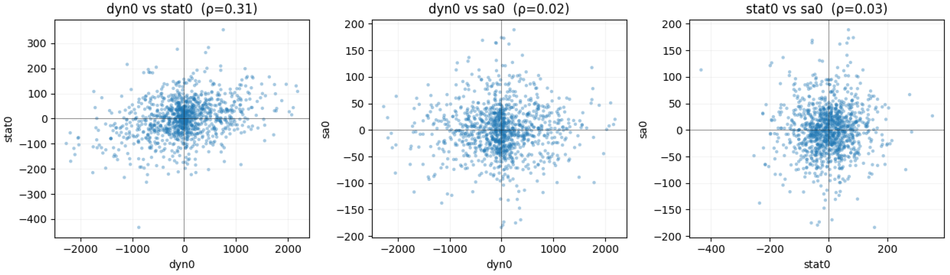
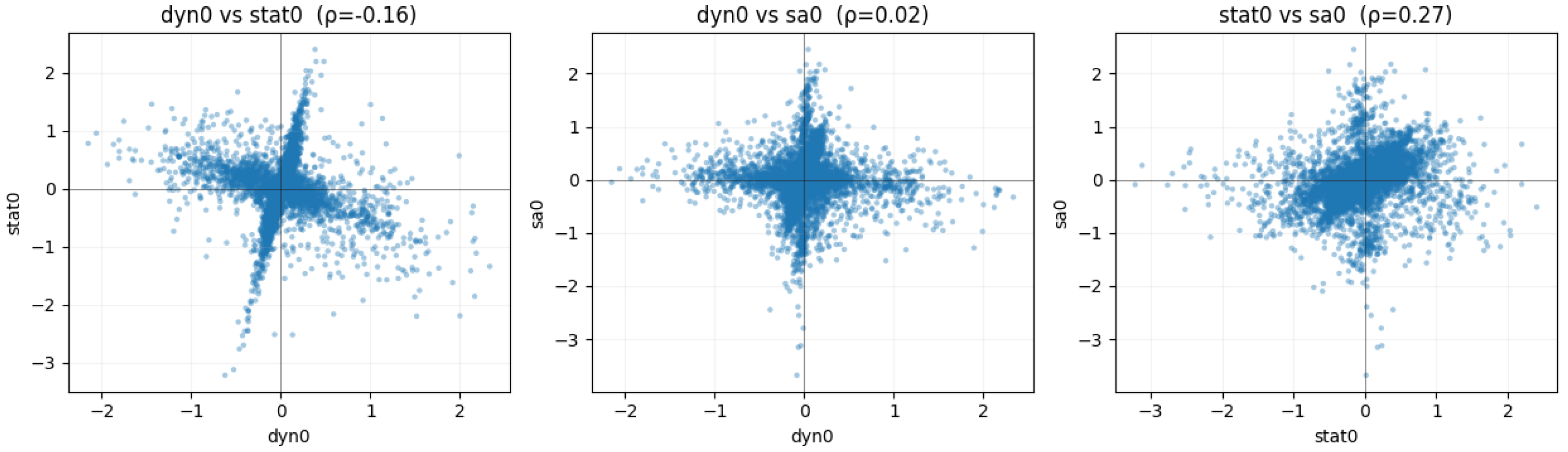
The diffusion matrix is specified to be diagonal (Section 3.4), which presumes that the driving noises of the factors are mutually uncorrelated. Figure 16 shows the pairwise scatter of the factor residuals together with their Pearson correlations. The dynamic and static-arbitrage residuals are essentially uncorrelated ( ρ = 0.02 ), and the dynamic and statistical residuals are only weakly correlated ( ρ = 0.16 ), whereas the statistical and static-arbitrage residuals retain a moderate correlation ( ρ = 0.27 ). The cross- or star-shaped point clouds, with mass concentrated along the axes and heavy tails, are consistent with weakly dependent, leptokurtic marginals. The diagonal specification is thus broadly supported but not exact over the week: the residual correlation is larger than in the 24 h analysis of Section 4.4.2, suggesting that as the sample spans more regimes, a small amount of cross-factor dependence—chiefly between the statistical and static-arbitrage factors—is left unmodelled by the diagonal diffusion.

5. Applications

This section considers two fundamental downstream applications: hedging and risk management, in the form of Value-at-Risk (VaR). These represent the most immediate and practically meaningful uses of a market pricing model. Both tasks provide direct validation of the model’s ability to capture market dynamics: hedging evaluates how well the learned dynamics can replicate real-world sensitivities and risk exposures, while VaR assesses the model’s capacity to simulate realistic loss distributions under stochastic evolution. However, this is not to say that this is an exhaustive list of the model’s capabilities, as it provides a complete stochastic representation of how the implied volatility and option prices evolve through time. In principle, this framework can be extended to a wide range of quantitative finance tasks—including scenario generation, risk-neutral valuation, stress testing, derivative portfolio simulation, and even data-driven model calibration or the discovery of latent market factors.

5.1. Market Simulation and VaR

Cohen et al. (2023b) detail the methodology on how to create VaR estimates for option portfolios using neural SDE market models. In essence, the neural SDE is a generative model, meaning that it can simulate the learned Ξ market factors. Via a factor decoding process (i.e., moving from the low-dimensional factor space back to a higher-dimensional option surface), simulated prices for various option portfolios can be obtained. As we now have a distribution of potential returns for the options on our defined liquid lattice, we can naturally compute VaR estimates (and hence other risk metrics, such as expected shortfall) using this distribution.

5.1.1. Market Simulation Methodology

Let Ξ t R d denote the vector of latent market factors, evolved according to the trained neural SDE:
d Ξ t = μ θ ( Ξ t ) d t + σ ϕ ( Ξ t ) d W t , σ ϕ ( Ξ t ) : = diag ( σ ( Ξ t ) ) 0 ,
where μ θ and σ ϕ represent the learned drift and diffusion networks, and W t is a standard Brownian motion. During simulation, we again ensure that the factor process Ξ t remains within the static-arbitrage polytope defined by the half-space constraints:
P arb = { Ξ t A G Ξ t b G } .
For each face i of the polytope, define the signed distance
ρ i ( Ξ t ) = A G , i Ξ t b G , i , i = 1 , , m ,
which measures proximity to the ith constraint boundary.
As before, we apply a smooth Lipschitz function φ σ : R + [ 0 , 1 ] to modulate the effective diffusion near the boundary:
ε i ( Ξ t ) = φ σ ( ρ i ( Ξ t ) ) = ρ i ( Ξ t ) 1 + ρ i ( Ξ t ) .
Let Q ( Ξ t ) be an orthonormal basis spanning the k most active faces (smallest ρ i ), and define
P ( Ξ t ) = Q ( Ξ t ) diag ( ε ( Ξ t ) ) 0 0 I d k Q ( Ξ t ) .
The effective diffusion is then given by
σ eff ( Ξ t ) = diag s ( Ξ t ) σ ( Ξ t ) ,
where s ( Ξ t ) [ 0 , 1 ] d are elementwise shrink coefficients matching P ( Ξ t ) σ ( Ξ t ) in covariance. By construction, the normal component A G , i Γ eff ( Ξ t ) A G , i 0 as ρ i ( Ξ t ) 0 , satisfying the diffusion non-attainability condition.
Again following our previous procedure, a smooth correction is added to ensure the drift points inward at the boundary. Define a Lipschitz function φ μ ( ρ ) = 1 1 + ρ and inward directions d i associated with each active face normal A G , i . The corrected drift is:
μ corr ( Ξ t ) = μ θ ( Ξ t ) + i I ( Ξ t ) ω i ( Ξ t ) d i , ω i ( Ξ t ) = A G , i μ θ ( Ξ t ) φ μ ( ρ i ( Ξ t ) ) + d i , A G , i ,
ensuring A G , i μ corr ( Ξ t ) 0 along all active faces.
Given a discretisation step Δ t , each Euler–Maruyama step evolves as:
Ξ t + Δ t = Ξ t + μ corr ( Ξ t ) Δ t + σ eff ( Ξ t ) Δ t ε t , ε t N ( 0 , I d ) .
Running B Monte Carlo paths of Ξ t generates a sample distribution of factor evolutions { Ξ t ( b ) } b = 1 B .

5.1.2. VaR of Option Portfolios

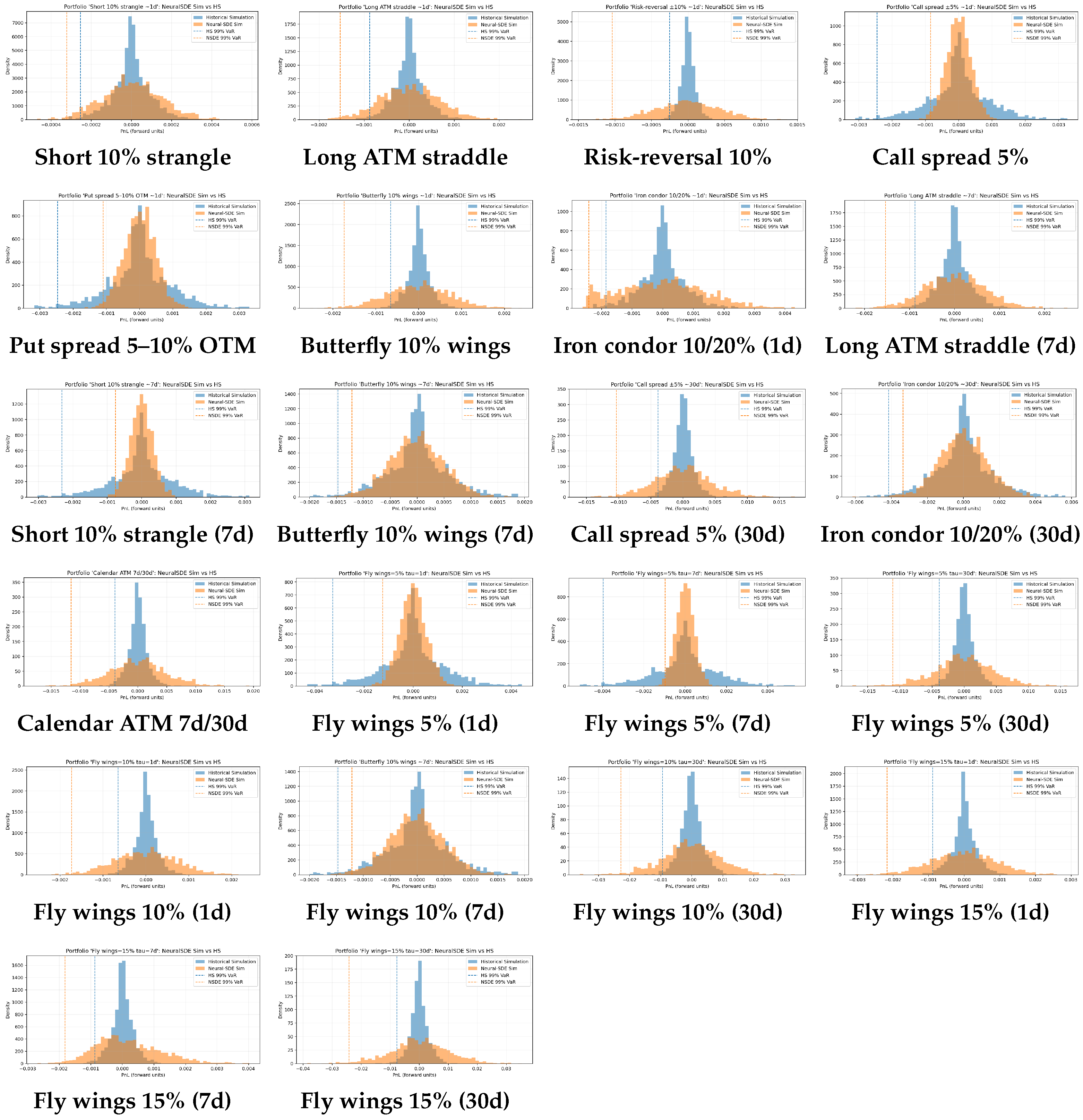
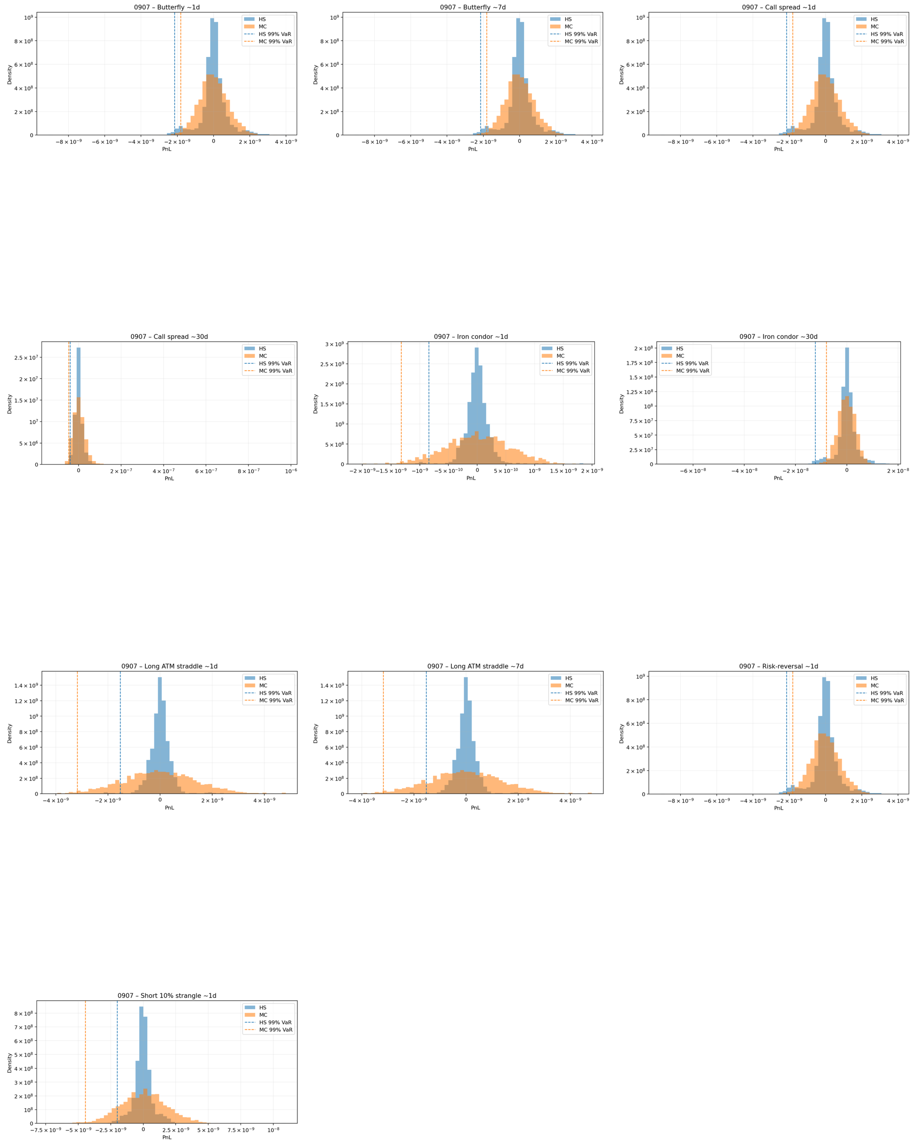
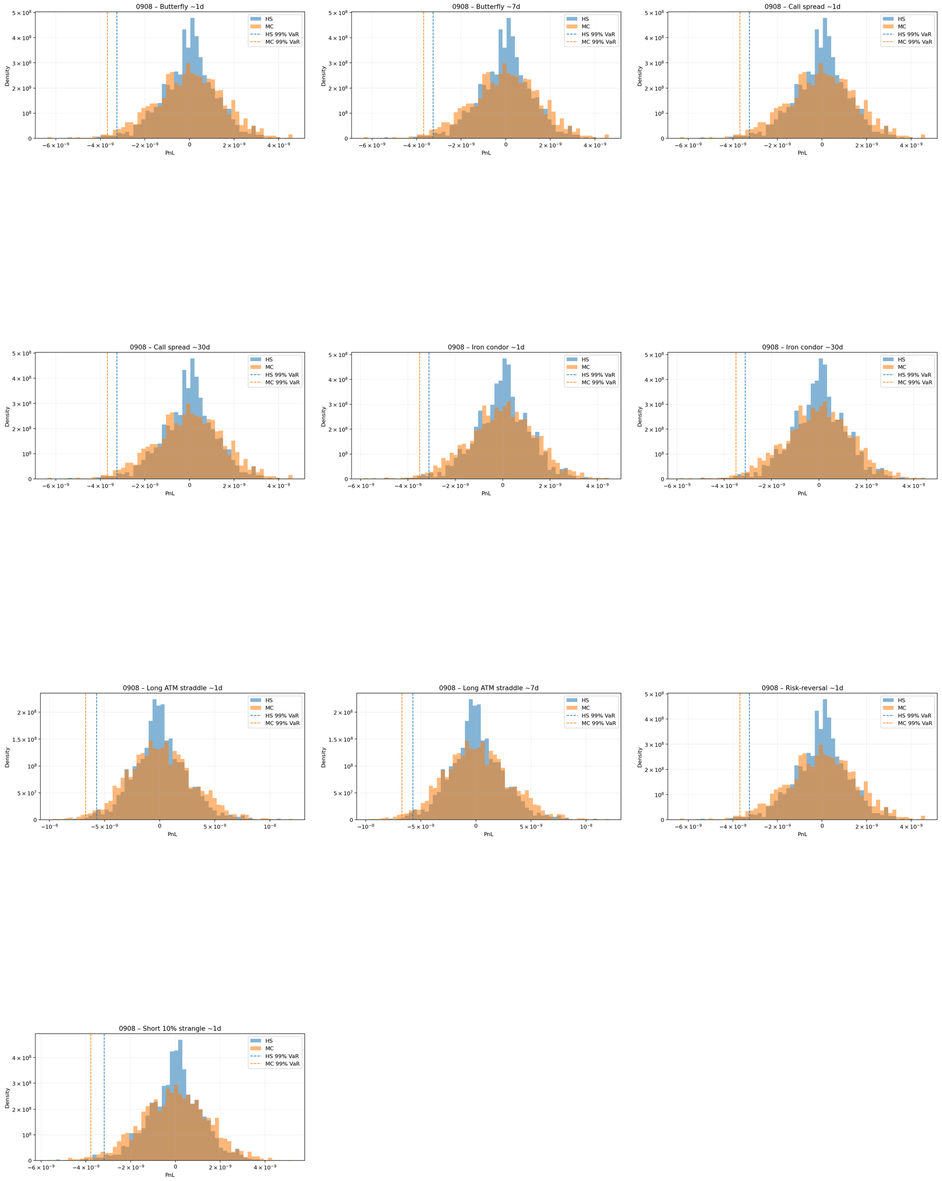
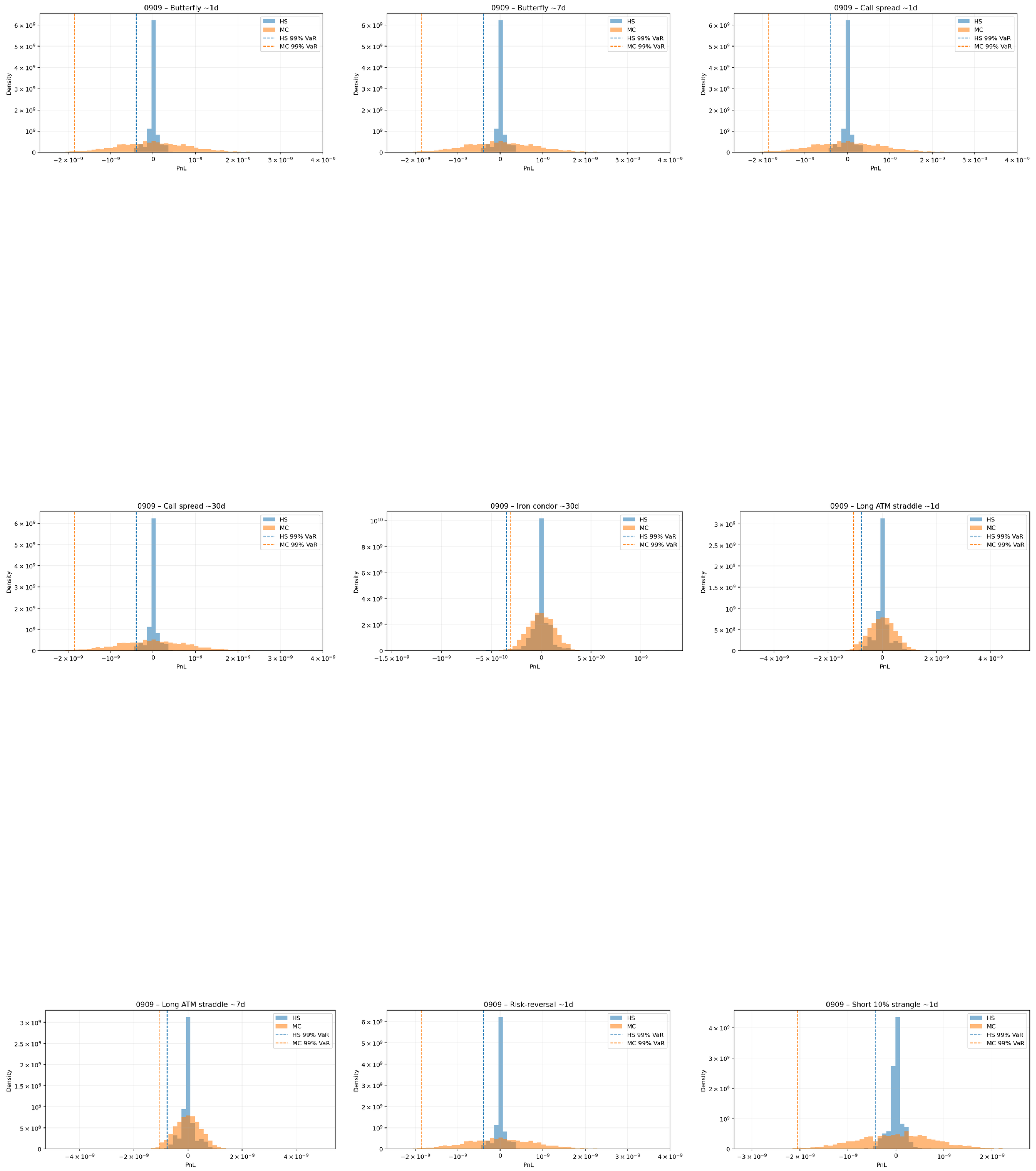
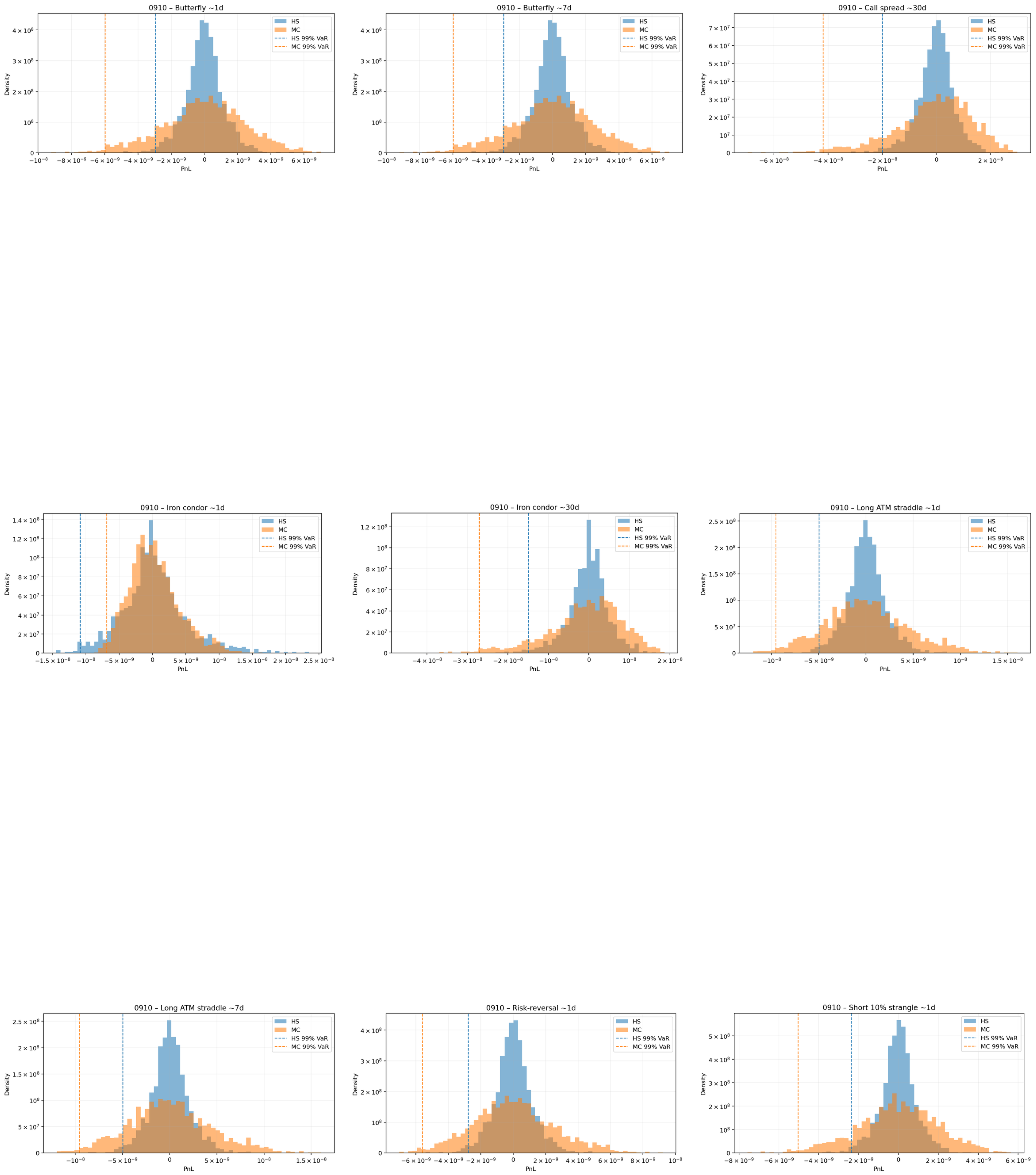
Table 1 presents VaR results for various option portfolios, for both the neural SDE simulation and a standard historical simulation approach.
The results in Table 1 show that across all portfolios, the neural SDE simulated Value-at-Risk (VaR) estimates are consistently higher in magnitude than those obtained via historical simulation. This indicates that the neural SDE captures fatter tails and greater short-term variability in the factor dynamics, reflecting more realistic risk in high-frequency markets, such as cryptocurrency options. The largest VaR differences appear in short-maturity, short-volatility positions (e.g., short strangles and short condors), where non-linear payoffs are most sensitive to volatility clustering and jump-like behaviour. Conversely, for longer-dated or more balanced portfolios (e.g., butterflies or calendar spreads), the neural SDE and historical methods yield more comparable results, suggesting that the learned diffusion smooths risk over longer horizons.
Plotting a few examples of loss distributions in Figure 17 and comparing against a distribution from historical simulation, we can see that the neural SDE does indeed provide a different distribution. We interpret these as reflecting data-driven and arbitrage-consistent dynamics of the underlying surface. Noting that traditional historical simulation approaches assume that options, or market factors, move individually, however, we know that options move as a surface with constraints to their state, as discussed in Section 2.2. The historical simulation approach taken here, in comparison, is a simulation of the market factors; that is to say, we look at the historical distribution of returns we have (in the test period) and simulate returns by sampling from this distribution. Option prices/portfolios are simulated by a factor decoding process.

5.2. Hedging of Option Portfolios

Cohen et al. (2022) highlight how we can use the learned model to hedge a portfolio of options. While their work presents both sensitivity-based hedging and minimum-variance (MV) hedging, in our case, the applications to cryptocurrency options will be focused on the MV hedge, as it directly uses the learned neural SDE model, whereas the sensitivity-based hedge only uses the factor representation of option prices.

5.2.1. Minimum-Variance Hedging

Let Ξ t R d denote the latent market factors driving the option surface, and recall the linear decoder from Section 3.4,
c ˜ ( Ξ t ) = G 0 + i = 1 d G i ξ i t = G 0 + M Ξ t , M R N × d ,
where M = [ G 1 G d ] is the loading matrix defined in Section 3.4. For a portfolio defined by node weights w R N , the portfolio’s factor exposure vector is given by
s = M w R d .
To first order, the one-step change in portfolio value is given by
Δ V t s Δ Ξ t , Δ Ξ t : = Ξ t + 1 Ξ t .
From the learned neural SDE model, the drift and diffusion functions μ θ ( Ξ t ) and σ ϕ ( Ξ t ) define the instantaneous covariance of the latent factors as
Σ t base = σ ϕ ( Ξ t ) σ ϕ ( Ξ t ) .
To ensure that this covariance structure respects the static-arbitrage geometry defined by the polytope constraints A G Ξ t b G , we apply a state-dependent linear map Ω t that shrinks the diffusion along the active boundary directions, as detailed in Equation (16). The resulting adjusted covariance is
Σ t = Ω t Σ t base Ω t .
This procedure ensures that factor dynamics remain within the feasible arbitrage-free region during simulation and hedging.
Now, consider a set of k hedging instruments indexed by H = { j 1 , , j k } . Let B R d × k denote their factor exposures,
B : = M : , H .
The static minimum-variance (MV) hedge solves
u = arg min u R k Var ( s B u ) Δ Ξ t = B Σ ¯ B 1 B Σ ¯ s ,
where Σ ¯ = 1 T 1 t Σ t is the time-averaged model-implied factor covariance. A dynamic version of this hedge recomputes u t at each time step, according to
u t = B Σ t B 1 B Σ t s ,
yielding time-varying hedge weights that evolve consistently with the latent factor covariance implied by the neural SDE. In practice, the Σ t matrices are computed per step using the endogenous shrinkage Ω t and the trained model parameters ( θ , ϕ ) .

5.2.2. Hedging an Example Portfolio (a 30-Day ATM Option)

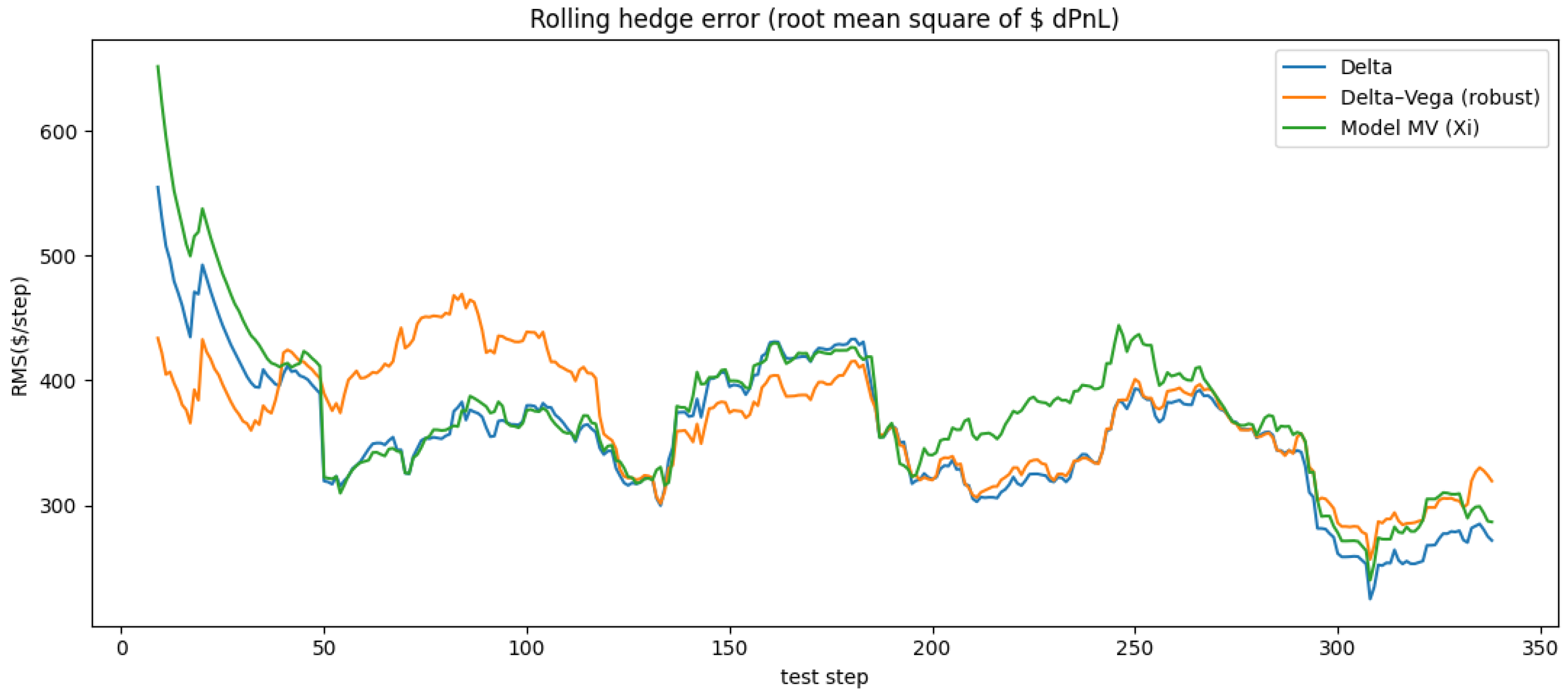
We present hedging results for a portfolio consisting of an at-the-money option with a 30-day expiry. Figure 18 showcases the root mean squared error of the neural SDE MV hedge compared with standard Black–Scholes delta and delta-vega hedging.
While we cannot say that the MV hedging procedure from the learned neural SDE model outperforms the delta or delta-vega hedge, we can state that it is comparable to these traditional hedging methods. These hedging results on cryptocurrency are similar to the results from Cohen et al. (2022), who present hedging results from traditional equities and forex markets.

6. Limitations and Conclusions

6.1. Limitations of Modelling Methods

There are several limitations that one should consider with this neural SDE modelling choice. First, the neural SDE model assumes continuous-diffusion dynamics and therefore will not reflect jumps. The data-driven nature of the neural SDEs will, to some extent, allow it to adapt to volatility clustering and heavy-tailed distributions over longer time periods, but at the scale of each single time step, the approximation by Euler/Maruyama discretisation introduces an implicit assumption of Gaussianity. A full Lévy or jump-diffusion extension of the approach presented in the present paper may be a fruitful avenue of further investigation, as it may yield a more realistic specification. Second, training was limited to a single day and a single week of data due to computational and storage constraints; extending the analysis across multiple weeks could provide stronger statistical validation. Third, although static-arbitrage constraints are enforced strictly, dynamic arbitrage is only minimised, not eliminated, and a theoretical guarantee of global consistency across time remains an open challenge. Finally, the current modelling requires a fixed-factor dimension and lattice shape. Future research should aim to address these limitations.

6.2. Conclusions

This paper provides a synthesis of several methods in the literature and presents a pipeline that takes in raw option quotes and produces a non-parametric model for the entire option surface. The presented neural SDE model adheres to static-arbitrage constraints, and the applications to risk management and hedging have been showcased. One can conclude that combining machine learning with known financial laws, e.g., arbitrage constraints, can provide non-parametric alternatives to traditional models.
Our results demonstrate the feasibility of applying the arbitrage-free neural SDE market model of Cohen et al. (2023a) to an entirely new asset class—high-frequency cryptocurrency options—where the microstructure and volatility regimes differ substantially from traditional markets. In particular, this extends the model’s applicability to ultra-high-frequency data, developing pre-processing methods for constructing static liquid lattices and repairing arbitrage in sparse intraday panels. The elements brought together here form a complete pipeline from raw data to an operational, data-driven, arbitrage-free simulator of the Bitcoin options market.

Author Contributions

Conceptualisation, A.S. and E.S.; methodology, A.S.; software, A.S.; validation, A.S. and E.S.; formal analysis, A.S.; investigation, A.S. and E.S.; resources, A.S.; data curation, A.S.; writing—original draft preparation, A.S.; writing—review and editing, E.S.; visualisation, A.S.; supervision, E.S. All authors have read and agreed to the published version of the manuscript.

Funding

This research received no external funding.

Data Availability Statement

The data were obtained from Deribit and are made publicly available by Deribit via https://www.deribit.com/ (accessed on 19 June 2026). To reproduce the results reported in the present paper, historical Deribit data can be accessed via the Deribit API; see https://support.deribit.com/hc/en-us/articles/25973087226909-Accessing-historical-trades-and-orders-using-API (accessed on 19 June 2026).

Acknowledgments

The authors are grateful for fruitful discussions with Mark Capogreco and for constructive suggestions provided by three anonymous reviewers. The usual disclaimers apply.

Conflicts of Interest

The authors declare no conflicts of interest.

Appendix A. Arbitrage-Free Surfaces Between the Bid and Ask Spread

Consider the interpolated price vector
c k = ( 1 k ) b raw + k a raw ,
for a scale parameter k [ 0 , 1 ] . This represents a convex combination between the raw bid price vector b raw (when k = 0 ) and the raw ask price vector a raw (when k = 1 ), interpolating uniformly across all nodes.
We require that this interpolated vector satisfies the static-arbitrage and non-negativity constraints:
A c k 0 , c k 0 ,
where A R R × n encodes the linear inequalities enforcing monotonicity in maturity, monotonicity and convexity in moneyness, and non-negativity across all lattice points.
Substituting Equation (A1) into the constraints gives:
( 1 k ) A b raw + k A a raw 0 .
Each row r of this matrix inequality corresponds to a scalar linear constraint:
( 1 k ) ( A b raw ) r + k ( A a raw ) r 0 , r = 1 , , R .
Each inequality in (A4) defines a half-space constraint on k, restricting k to one side of a threshold value within the interval [ 0 , 1 ] . Taken together, these R inequalities define a closed feasible interval:
[ k min , k max ] [ 0 , 1 ] .
If this interval is non-empty, i.e., k min k max , then there exists at least one uniform interpolation c k between the bid and ask vectors that is arbitrage-free. The endpoints of the feasible interval can be computed explicitly by solving two simple linear programs:
k min = arg min 0 k 1 k s . t . ( 1 k ) A b raw + k A a raw 0 ,
k max = arg max 0 k 1 k s . t . ( 1 k ) A b raw + k A a raw 0 .
These solutions yield the exact bounds on k ensuring arbitrage-free uniform interpolation within the observed bid–ask spread.
Interpretation. Geometrically, each inequality in Equation (A3) defines a half-space in the one-dimensional variable k, restricting k to values for which the interpolated surface c k remains within the arbitrage-free region defined by A c k 0 . The intersection of these half-spaces yields the feasible interval [ k min , k max ] , within which all convex combinations of bid and ask prices satisfy the static no-arbitrage constraints. If this interval is non-empty, it implies that the observed bid–ask quotes are internally consistent with at least one arbitrage-free price surface. Conversely, an empty interval indicates that no uniform interpolation between bids and asks can satisfy all no-arbitrage inequalities simultaneously, signalling inconsistency or microstructure noise in the quoted market data.

Appendix B. Drift Restrictions, Dynamic Arbitrage and the “z-Factor”

This appendix serves as an explanation of how we minimise dynamic arbitrage, as defined in Section 2.3, in the reconstructed option prices. Appendix A in Cohen et al. (2023a) gives a detailed derivation for this. For the reader’s convenience, this derivation is summarised here, with additional commentary on the application to the Deribit data.
First, note that it is a sufficient condition for the absence of arbitrage (dynamic and static) that there exists an equivalent martingale measure, such that the discounted price process of any tradable instrument is a local martingale Q . For an option with maturity T and strike K, this implies the Heath–Jarrow–Morton (HJM)-type drift restriction:
ν t ( T , K ) · ϕ t = η t ( T , K ) + ν 0 , t ( T , K ) γ t ,
where η t ( T , K ) and ν t ( T , K ) are respectively the drift and diffusion of the option price process under the physical measure P , ϕ t is the market price of the risk vector, and γ t is the volatility of the underlying process.

Appendix B.1. Drift of the Option Surface Under the Physical Measure

From the factor representation of normalised call prices:
c ˜ t ( τ , m ) = G 0 ( τ , m ) + i = 1 d ξ i , t G i ( τ , m ) ,
where τ = T t and m = log ( K / F t ) , applying Itô’s lemma yields the differential of the call surface evaluated along the moving coordinates ( τ t , m t ) :
d c ˜ t = i G i ( τ t , m t ) d ξ i , t + c ˜ t τ d τ t + c ˜ t m d m t + 1 2 2 c ˜ t m 2 d m t .
Substituting d τ t = d t , d m t = ( α t + 1 2 γ t 2 ) d t γ t d W 0 , t , and d m t = γ t 2 d t gives the drift of surface evolution:
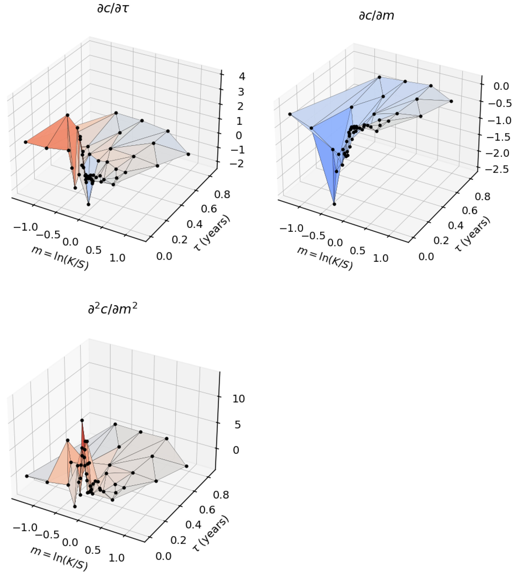
d c ˜ t d t = c ˜ t τ 1 2 γ t 2 c ˜ t m + 1 2 γ t 2 2 c ˜ t m 2 + i μ i , t G i ( τ t , m t ) .

Appendix B.2. The Infinitesimal Drift Operator and the z-Factor

We define the deterministic differential operator
Z : = τ 1 2 γ t 2 m + 1 2 γ t 2 2 m 2 ,
and apply it to the reconstructed option surface to obtain the z-factor:
z t = Z [ c ˜ t ] ( τ t , m t ) .
This represents the infinitesimal deterministic drift of the option surface induced by the decay of time to maturity and the diffusion of moneyness. Intuitively, z t describes how the option surface should evolve in ( τ , m ) -space in order to remain dynamically arbitrage-free.

Appendix B.3. Dynamic No-Arbitrage Under the Basis Expansion

Under the basis expansion of Equation (A11), the HJM drift restriction becomes:
G μ t z t = G σ t ψ t ,
where μ t and σ t are respectively the drift and diffusion coefficients of the factor process d ξ t = μ t d t + σ t d W t , and ψ t is the vector of market prices of risk. Equation (A14) states that, up to a change in measure, the observed drift of the factors G μ t should be explainable by the deterministic surface drift z t and the model’s diffusion structure G σ t .

Appendix B.4. Principal Component Analysis of the z-Factor

We compute z t empirically for each observation of the reconstructed surface and perform principal component analysis (PCA) over its temporal evolution. The PCA decomposes the variability in z t into orthogonal modes corresponding to consistent directions of deterministic surface motion (e.g., level, skew, curvature shifts). If the market is dynamically arbitrage-free, these principal directions should align closely with the factor basis { G i } .
Residual components of z t that are orthogonal to span { G i } indicate systematic drifts of the surface that are not representable by the model’s factors, implying violations of the HJM drift restriction. By quantifying the variance explained by the first d principal components of z t , we obtain a diagnostic of the extent to which the neural SDE factor model captures the dynamically consistent evolution of the option surface.

Appendix B.5. Minimising Dynamic Arbitrage

By training the model and selecting factor structures such that the leading principal components of z t align with the learned factors G i , we effectively minimise the unexplained component of the HJM drift restriction. This ensures that the model-implied surface evolution under the physical measure P is as close as possible to one that admits an equivalent martingale measure Q , that is, the dynamic arbitrage in the model is minimised.

Appendix B.6. Empirical Computation of the “z-Factor”

While the work by Cohen et al. (2023a) uses splines to calculate the derivatives in (A12), we have access to high-frequency data, so we use finite-difference methods. The γ t parameter is computed by fitting an initial, “Stage 0”, neural SDE to just the underlying process.
Our estimated surface derivatives are jagged/irregular due to the sparsity of our lattice. However, they do approximately resemble the surface derivatives presented by Cohen et al. (2023a) in shape.
Figure A1. Surface derivatives at t = 0, 22 May 2025 Deribit call options.
Risks 14 00151 g0a1

Appendix C. Training at Ultra-High-Frequency Intervals

The results in this paper have been for prices, for options and the underlying asset, that have been aggregated to minute increments. This appendix provides some results and commentary for training the neural SDE model on raw, un-aggregated increments. This means that each unique timestamp is at the sub-second level. Figure 1 elucidates the distribution of the interval length without any resampling/aggregation of prices. We can see that the majority of sampled intervals from Deribit are less than one second (sub-second level intervals).
Analysing Figure A2 and Figure A3 we can see that although the loss curve looks to be converging, the model does not seem to be respecting the Gaussian transition from our Euler–Maruyama training assumption. The tails on the QQ plots for the residuals show clear flat tails, suggesting that extreme values for transitions (both negative and positive) are more common, or higher in intensity, than what one would expect for the assumption of Gaussianity. One can speculate that this is due to the presence of microstructure noise at the lowest time-scales (Bandi and Russell 2006).
Figure A2. QQ plots of 3 factors at HF.
Risks 14 00151 g0a2
Figure A3. Loss curve training at HF (with constraints).
Risks 14 00151 g0a3

Appendix D. Alternative Likelihoods for Training

Here we report on an attempt to model the transition probabilities more accurately using a different likelihood parameterisation. To estimate the parameters of our neural SDE, we employ a quasi-likelihood approach inspired by Aït-Sahalia’s expansion for diffusion transition densities (Aït-Sahalia 2002). The true transition density of a non-linear stochastic differential equation,
d Y t = μ ( Y t ) d t + σ ( Y t ) d W t ,
is generally intractable except for a few special cases. Aït-Sahalia proposed a first-order approximation based on the Lamperti transformation, which locally linearises the diffusion coefficient. Defining the transform
Z t = Y 1 σ ( y ) d y ,
the dynamics of Z t can be written approximately as
d Z t μ ( Y t ) σ ( Y t ) 1 2 σ ( Y t ) d t + d W t .
This results in an approximate Gaussian transition density for Z t + Δ t conditional on Z t ,
p ( Y t + Δ t | Y t ) N Z t + Δ t ; Z t + μ L ( Y t ) Δ t , Δ t · | Z / Y t + Δ t | ,
where μ L ( Y t ) = μ ( Y t ) σ ( Y t ) 1 2 σ ( Y t ) and the Jacobian term log | Z / Y t + Δ t | = log σ ( Y t + Δ t ) corrects for the non-linear transformation.
In implementation,4 the networks μ θ ( · ) and σ ϕ ( · ) parameterise the drift and diffusion, and the loss is given by the sum of per-step negative log-likelihoods of this approximate density. Compared to the standard Euler–Maruyama Gaussian likelihood, which assumes locally constant diffusion, the Aït-Sahalia quasi-likelihood explicitly accounts for the spatial variation in σ ( Y t ) through its derivative σ ( Y t ) , improving statistical efficiency and potentially providing a more accurate approximation of the true SDE transition law while remaining consistent with the Euler–Maruyama discretisation framework.
However, when training a neural SDE market model with this transition as the loss, at the native high-frequency intervals, we can see that the QQ plots still show clear fat tails; see Figure A4. This suggests that the noise at high frequency is still too large for the Gaussian assumption to hold, even when including spatial derivatives for the diffusion.
Figure A4. QQ Plots for quasi-likelihood training at native high-frequency intervals.
Risks 14 00151 g0a4

Appendix E. Neural Network Architecture

We model a diagonal Itô SDE d X t = f θ ( X t ) d t + diag g θ ( X t ) d W t , where the drift f θ : R p R p and diffusion amplitude g θ : R p R + p are small multi-layer perceptrons (MLPs). The baseline network (neural SDE) uses two parallel heads with identical depth: (i) the drift head is a two-layer MLP Linear ( p , 256 ) ReLU Linear ( 256 , p ) , and (ii) the diffusion head is Linear ( p , 256 ) ReLU Linear ( 256 , p ) Softplus , where the Softplus enforces g θ ( x ) > 0 component-wise. Thus, both architectures are compact two-layer multi-layer perceptrons with ReLU-hidden activations and Softplus on diffusion, with the shrink variant inserting a geometric diffusion contraction that preserves positivity and encodes static constraints.
The neural SDE architecture used for the latent factor dynamics is visualised in Figure A5. The input is the factor state Ξ t R d . The drift network outputs μ θ ( Ξ t , t ) , and the diffusion network outputs the component-wise non-negative diagonal diffusion amplitude σ ϕ ( Ξ t , t ) , with Softplus enforcing positivity. Note that in our implementation of neural SDEs, we have a final layer that constrains both the drift and diffusion to enforce no-arbitrage boundaries.
Figure A5. Neural SDE architecture for latent factor dynamics.
Risks 14 00151 g0a5

Appendix F. Factor-Lattice Sensitivity Analysis

As discussed in Section 3.2, the liquid lattice N is constructed heuristically from the empirical liquidity profile, and Cohen et al. (2023a) likewise choose the lattice shape by hand. Because the factor loadings of Section 3.4 are estimated on this lattice, it is natural to ask whether the recovered factor representation is an intrinsic feature of the surface dynamics or an artefact of the particular nodes chosen. This appendix reports a controlled sensitivity study: we hold the arbitrage-repaired data fixed for a single representative trading day, the llth of September, and vary only the set of lattice nodes on which the factors are decoded, then measure how far the resulting loadings move.

Appendix F.1. Experimental Design

Recall the linear factor representation (9), c ˜ = G 0 + M Ξ t with M = [ G dyn G stat G sa ] . For each candidate node set (“lattice variant”) L N we re-estimate the two principal component blocks of Algorithm 1 of Cohen et al. (2023a), exactly as in Section 3.4, restricted to the columns indexed by L . Writing Z ( L ) R ( L 1 ) × | L | for the time series of the z-factor of Appendix B,
z t = τ 1 2 γ t 2 m + 1 2 γ t 2 2 m 2 c ˜ t ,
evaluated on the nodes of L and column-centred, the dynamic loadings { G i dyn } are taken to be its leading right singular vectors, while the statistical loadings { G i stat } are the leading right singular vectors of the price residual that remains after the dynamic block is projected out. The static-arbitrage factor G sa is excluded from the comparison: it is defined by feasibility against the constraint matrix A, rather than by the variance structure of the surface, and would require re-deriving A on each L .
We consider five deterministic variants: the full baseline lattice ( | N | = 22 nodes); a maturity-coarsened grid (every second maturity removed); a moneyness-coarsened grid (every second strike per maturity removed); a wing-trimmed grid (deep in/out-of-the-money nodes removed); and a delta-spaced grid in which nodes are placed at uniform option-delta targets in place of the baseline’s moneyness percentiles. The reduced lattices retain between 13 and 16 nodes. To probe stability under unstructured perturbations we additionally draw 100 random retentions of 70 % of the nodes.

Appendix F.2. Comparison Metrics

The factors are identified only up to the sign, permutation and rotation, so an entrywise comparison of loadings is not meaningful. We therefore interpolate every loading vector onto a common ( τ , m ) grid, denote the result G ^ i ( L ) , and sign- and permutation-align each variant to the baseline by maximising the absolute cosine. For two aligned loadings we report the cosine similarity
ρ G ^ i ( L ) , G ^ i ( N ) = | G ^ i ( L ) , G ^ i ( N ) | G ^ i ( L ) G ^ i ( N ) [ 0 , 1 ] .
Because an individual factor may rotate within the spanned subspace without changing what the model can represent, our primary, rotation-invariant criterion is the overlap of the factor subspaces. Let G ( L ) = span { G ^ i ( L ) } have orthonormal basis Q ( L ) . The canonical correlations between G ( L ) and the baseline subspace G ( N ) are the singular values
cos θ k = σ k Q ( L ) Q ( N ) , k = 1 , , d dyn + d stat ,
where { θ k } are the principal angles between the subspaces; min k cos θ k = 1 indicates that the two lattices span an identical factor subspace. We summarise robustness by the minimum and mean canonical correlation.

Appendix F.3. Results

Figure A6 shows the aligned dynamic and statistical loadings as surfaces over maturity and log-moneyness for each variant, and Figure A7 shows the corresponding differences relative to the baseline lattice. Two regimes are evident: variants that preserve node density and coverage—the delta-spaced and wing-trimmed grids—reproduce the baseline loadings almost exactly, with small and spatially incoherent residuals, whereas coarsening the grid produces large, structured differences that are most pronounced for the moneyness-coarsened lattice. The per-factor cosine similarities of Figure A8 quantify this: the delta-spaced and wing-trimmed lattices attain cosines of 0.98 1.00 ; the maturity-coarsened lattice gives 0.75 for the dynamic and 0.71 for the statistical factor; and while the moneyness-coarsened lattice leaves the dynamic factor largely intact (cosine 0.90 ), it collapses the statistical factor to a cosine of 0.25 , reflecting the loss of the smile curvature encoded by the discarded strikes. The rotation-invariant subspace diagnostic of Figure A9 tells the same story at the level of the spanned space, with minimum canonical correlations of 0.98 1.00 for the density-preserving variants, 0.70 for the maturity-coarsened lattice, and 0.22 for the moneyness-coarsened lattice.
A clear hierarchy emerges between the factors. Under the 100 random 70 % retentions (Figure A10), the leading dynamic (level/term-structure) factor remains tightly concentrated near the baseline—median cosine 0.99 , interquartile range above 0.91 , with only an isolated draw near 0.73 —whereas the statistical factor is markedly dispersed, with a median of ≈0.88 and a lower tail reaching 0.25 . Consistently, Figure A11 shows that the share of variance attributed to each factor shifts across lattices and that the two factors’ explained-variance ranks can reorder (for the maturity-coarsened lattice, the statistical factor explains more variance than the dynamic factor), so that the statistical factor behaves in part as an artefact of the specific node set rather than as a stable market mode.
Taken together, the factor representation is robust to the rule used to place a given set of liquid nodes—including a switch from moneyness to delta spacing and the removal of illiquid wing nodes—but sensitive to node density and coverage, particularly in the moneyness direction. We therefore regard inferences that rest on the dominant dynamic factor as transferable across reasonable lattice choices, while analyses that rely on higher-order factors should either fix the lattice density or report this sensitivity explicitly. Finally, we emphasise that this experiment varies the lattice on fixed data; comparing factors decoded on genuinely different days would additionally confound lattice geometry with the prevailing market regime, and the related degeneracy of the factor geometry on sparse single-day lattices is treated separately.
Figure A6. Dynamic ( G dyn , top) and statistical ( G stat , bottom) factor loadings for each lattice variant, shown as surfaces over maturity (rows, in days) and log-moneyness (horizontal axis, m = ln ( K / F ) ). Loadings are interpolated onto a common ( τ , m ) grid and sign/permutation-aligned to the baseline. The node count n of each lattice is indicated in the column title.
Risks 14 00151 g0a6
Figure A7. Difference between each variant’s aligned loadings and the baseline-lattice loadings, G ^ i ( L ) G ^ i ( N ) , over maturity (rows) and log-moneyness (horizontal axis). Colour scales differ across columns to reveal structure; note, in particular, the order-of-magnitude smaller scale of the delta-spaced column.
Risks 14 00151 g0a7
Figure A8. Per-factor cosine similarity (A16) between each lattice variant and the baseline, after sign and permutation alignment (a value of 1 denotes an identical loading direction).
Risks 14 00151 g0a8
Figure A9. Subspace overlap between each variant and the baseline, measured by the canonical correlations (A17) (mean and minimum over the principal angles). A minimum canonical correlation of 1 indicates that the variant spans the same factor subspace as the baseline lattice.
Risks 14 00151 g0a9
Figure A10. Stability of the factor loadings under 100 random retentions of 70 % of the lattice nodes. Boxplots show the distribution of the per-factor cosine similarity to the baseline; the dynamic factor is tightly concentrated near unity, whereas the statistical factor is dispersed with a heavy lower tail.
Risks 14 00151 g0a10
Figure A11. Per-factor explained-variance ratio across the lattice variants. The share of variance attributed to each factor shifts with the lattice, and the dynamic and statistical ranks reorder for the maturity-coarsened grid.
Risks 14 00151 g0a11

Appendix G. Extended VaR Analysis

This appendix extends the VaR analysis across the full September week’s worth of data. For each date, the neural SDE is retrained on that day’s option surface factor series and is used to generate simulated one-step portfolio return distributions out of sample. These are compared against the corresponding historical simulation return distributions for the same portfolio set.
While a proper VaR backtest is unfortunately infeasible due to data constraints, the figures below provide a distributional comparison between the neural SDE simulation and the historical simulation across several market days. The key observation is that the neural SDE return distributions are not simply reproductions of the historical simulation distributions. Across dates and portfolios, the simulated distributions often differ in dispersion, tail behaviour, and skewness. The historical return distributions also change across days, indicating that the comparison is sensitive to the market conditions in each daily training sample.
Figure A12. Extended VaR return-distribution comparison for 7 September 2025.
Risks 14 00151 g0a12
Figure A13. Extended VaR return-distribution comparison for 8 September 2025.
Risks 14 00151 g0a13
Figure A14. Extended VaR return-distribution comparison for 9 September 2025.
Risks 14 00151 g0a14
Figure A15. Extended VaR return-distribution comparison for 10 September 2025.
Risks 14 00151 g0a15
Figure A16. Extended VaR return-distribution comparison for 11 September 2025.
Risks 14 00151 g0a16
Figure A17. Extended VaR return-distribution comparison for 12 September 2025.
Risks 14 00151 g0a17
Figure A18. Extended VaR return-distribution comparison for 13 September 2025.
Risks 14 00151 g0a18
Figure A19. Extended VaR return-distribution comparison for 14 September 2025.
Risks 14 00151 g0a19

Notes

1
As recently documented, for example, in Franco and Laurini (2025).
2
An early example of the latter, using classical parametric models to fit cryptocurrency option surfaces, is Madan et al. (2019).
3
See https://www.deribit.com/ URL (last accessed on 19 June 2026)
4

References

  1. Ahmed, Mohamed Shaker, Ahmed A. El-Masry, Aktham I. Al-Maghyereh, and Satish Kumar. 2024. Cryptocurrency volatility: A review, synthesis, and research agenda. Research in International Business and Finance 71: 102472. [Google Scholar] [CrossRef]
  2. Aït-Sahalia, Yacine. 2002. Maximum likelihood estimation of discretely sampled diffusions: A closed-form approximation approach. Econometrica 70: 223–62. [Google Scholar] [CrossRef]
  3. Avordeh, Timothy King, Christopher Quaidoo, and Samuel Arthur. 2026. Hybrid machine learning and stochastic volatility models with blockchain data for high-frequency cryptocurrency trading. Discover Analytics 4: 5. [Google Scholar] [CrossRef]
  4. Bandi, Federico M., and Jeffrey R. Russell. 2006. Separating microstructure noise from volatility. Journal of Financial Economics 79: 655–92. [Google Scholar] [CrossRef]
  5. Black, Fischer, and Myron Scholes. 1973. The pricing of options and corporate liabilities. Journal of Political Economy 81: 637–54. [Google Scholar] [CrossRef]
  6. Breeden, Douglas T., and Robert H. Litzenberger. 1978. Prices of state-contingent claims implicit in option prices. Journal of Business 51: 621–51. [Google Scholar] [CrossRef]
  7. Buehler, Hans, Lukas Gonon, Josef Teichmann, and Ben Wood. 2019. Deep hedging. Quantitative Finance 19: 1271–91. [Google Scholar] [CrossRef]
  8. Caron, Richard J., John F. McDonald, and Carol M. Ponic. 1989. A degenerate extreme point strategy for the classification of linear constraints as redundant or necessary. Journal of Optimization Theory and Applications 62: 225–37. [Google Scholar] [CrossRef]
  9. Carr, Peter, and Dilip B. Madan. 2005. A note on sufficient conditions for no arbitrage. Finance Research Letters 2: 125–30. [Google Scholar] [CrossRef]
  10. Cohen, Samuel N., Christoph Reisinger, and Sheng Wang. 2020. Detecting and repairing arbitrage in traded option prices. Applied Mathematical Finance 27: 345–73. [Google Scholar] [CrossRef]
  11. Cohen, Samuel N., Christoph Reisinger, and Sheng Wang. 2022. Hedging option books using neural-SDE market models. arXiv arXiv:2205.15991. [Google Scholar] [CrossRef]
  12. Cohen, Samuel N., Christoph Reisinger, and Sheng Wang. 2023a. Arbitrage-free neural-sde market models. Applied Mathematical Finance 30: 1–46. [Google Scholar] [CrossRef]
  13. Cohen, Samuel N., Christoph Reisinger, and Sheng Wang. 2023b. Estimating risks of european option books using neural-sde market models. Journal of Computational Finance 26: 33–72. [Google Scholar]
  14. Cont, Rama, and Milena Vuletić. 2023. Simulation of arbitrage-free implied volatility surfaces. Applied Mathematical Finance 30: 94–121. [Google Scholar] [CrossRef]
  15. Cuchiero, Christa, Wahid Khosrawi, and Josef Teichmann. 2020. A generative adversarial network approach to calibration of local stochastic volatility models. Risks 8: 101. [Google Scholar] [CrossRef]
  16. Davis, Mark H. A., and David G. Hobson. 2007. The range of traded option prices. Mathematical Finance 17: 1–14. [Google Scholar] [CrossRef][Green Version]
  17. DeLise, Timothy. 2021. Neural Options Pricing. Ph.D. thesis, Universite de Montreal, Montreal, QC, Canada. [Google Scholar]
  18. Dempster, Arthur P., Nan M. Laird, and Donald B. Rubin. 1977. Maximum likelihood from incomplete data via the em algorithm. Journal of the Royal Statistical Society: Series B (Methodological) 39: 1–22. [Google Scholar] [CrossRef]
  19. Derman, Emanuel, and Iraj Kani. 1994. Riding on a smile. Risk 7: 32–39. [Google Scholar]
  20. Dhiman, Ashish, and Yibei Hu. 2023. Physics informed neural network for option pricing. arXiv arXiv:2312.06711. [Google Scholar]
  21. Dote-Pardo, Jairo, and María Teresa Espinosa-Jaramillo. 2026. A review of mathematical models for pricing, risk, and optimization in cryptocurrency analytics. Decision Analytics Journal 18: 100670. [Google Scholar] [CrossRef]
  22. Dridi, Naura, Lucas Drumetz, and Ronan Fablet. 2021. Learning stochastic dynamical systems with neural networks mimicking the euler-maruyama scheme. In 2021 29th European Signal Processing Conference (EUSIPCO). Piscataway: IEEE, pp. 1990–94. [Google Scholar]
  23. Dupire, Bruno. 1994. Pricing with a smile. Risk 7: 18–20. [Google Scholar]
  24. Fan, Lei, and Justin Sirignano. 2026. Machine learning methods for pricing financial derivatives. Quantitative Finance. [Google Scholar] [CrossRef]
  25. Franco, João Pedro M., and Márcio P. Laurini. 2025. Quantifying systemic risk in cryptocurrency markets: A high-frequency approach. International Review of Economics & Finance 102: 104214. [Google Scholar] [CrossRef]
  26. Friedman, Avner, and Mark A. Pinsky. 1973. Asymptotic stability and spiraling properties for solutions of stochastic equations. Transactions of the American Mathematical Society 186: 331–58. [Google Scholar] [CrossRef]
  27. Fukasawa, Masaaki. 2011. Asymptotic analysis for stochastic volatility: Martingale expansion. Finance and Stochastics 15: 635–54. [Google Scholar]
  28. Gatheral, Jim. 2011. The Volatility Surface: A Practitioner’s Guide. Hoboken: John Wiley & Sons. [Google Scholar]
  29. Gierjatowicz, Patryk, Marc Sabate Vidales, David Siska, Lukasz Szpruch, and Zan Zuric. 2022. Robust pricing and hedging via neural stochastic differential equations. Journal of Computational Finance 26: 1–32. [Google Scholar]
  30. Goodfellow, Ian, Jean Pouget-Abadie, Mehdi Mirza, Bing Xu, David Warde-Farley, Sherjil Ozair, Aaron Courville, and Yoshua Bengio. 2020. Generative adversarial networks. Communications of the ACM 63: 139–44. [Google Scholar] [CrossRef]
  31. Greff, Klaus, Sjoerd Van Steenkiste, and Jürgen Schmidhuber. 2017. Neural expectation maximization. Advances in Neural Information Processing Systems, 30. [Google Scholar]
  32. Hagan, Patrick S., Deep Kumar, Andrew S. Lesniewski, and Diana E. Woodward. 2002. Managing smile risk. The Best of Wilmott 1: 249–96. [Google Scholar]
  33. Harrison, J. Michael, and Stanley R. Pliska. 1981. Martingales and stochastic integrals in the theory of continuous trading. Stochastic Processes and Their Applications 11: 215–60. [Google Scholar] [CrossRef]
  34. Harrison, J. Michael, and Stanley R. Pliska. 1983. A stochastic calculus model of continuous trading: Complete markets. Stochastic Processes and Their Applications 15: 313–16. [Google Scholar] [CrossRef]
  35. Heath, David, Robert Jarrow, and Andrew Morton. 1992. Bond pricing and the term structure of interest rates: A new methodology for contingent claims valuation. Econometrica: Journal of the Econometric Society 60: 77–105. [Google Scholar] [CrossRef]
  36. Heston, Steven L. 1993. A closed-form solution for options with stochastic volatility with applications to bond and currency options. The Review of Financial Studies 6: 327–43. [Google Scholar] [CrossRef]
  37. Hutchinson, James M., Andrew W. Lo, and Tomaso Poggio. 1994. A nonparametric approach to pricing and hedging derivative securities via learning networks. The Journal of Finance 49: 851–89. [Google Scholar] [CrossRef]
  38. Kolm, Petter N., and Gordon Ritter. 2019. Dynamic replication and hedging: A reinforcement learning approach. The Journal of Financial Data Science 1: 159–71. [Google Scholar] [CrossRef]
  39. Lyons, Terry J. 1995. Uncertain volatility and the risk-free synthesis of derivatives. Applied Mathematical Finance 2: 117–33. [Google Scholar] [CrossRef]
  40. Madan, Dilip B., Sofie Reyners, and Wim Schoutens. 2019. Advanced model calibration on bitcoin options. Digital Finance 1: 117–37. [Google Scholar] [CrossRef]
  41. Phytides, Alexio. 2023. No-Arbitrage Option Pricing with Neural Sdes. Master’s thesis, University of Cape Town, Cape Town, South Africa. [Google Scholar]
  42. Roper, Michael, and Marek Rutkowski. 2009. On the relationship between the call price surface and the implied volatility surface close to expiry. International Journal of Theoretical and Applied Finance 12: 427–41. [Google Scholar] [CrossRef]
  43. Schönbucher, Philipp J. 1999. A market model for stochastic implied volatility. SSRN Electronic Journal. [Google Scholar] [CrossRef]
  44. Sutton, Richard S., and Andrew G. Barto. 1998. Reinforcement Learning: An Introduction. Cambridge: MIT Press, vol. 1. [Google Scholar]
  45. Tanios, Ramy. 2021. Physics Informed Neural Networks in Computational Finance. Master’s thesis, ETH Zurich, Zürich, Switzerland. [Google Scholar]
  46. Vuletić, Milena, and Rama Cont. 2024. Volgan: A generative model for arbitrage-free implied volatility surfaces. Applied Mathematical Finance 31: 203–38. [Google Scholar] [CrossRef] [PubMed]
  47. Wiese, Magnus, Lianjun Bai, Ben Wood, and Hans Buehler. 2019. Deep hedging: Learning to simulate equity option markets. arXiv arXiv:1911.01700. [Google Scholar]
  48. Wissel, Johannes Stefan. 2008. Arbitrage-Free Market Models for Liquid Options. Ph.D. thesis, ETH Zurich, Zürich, Switzerland. [Google Scholar]
Figure 1. Native high-frequency interval distribution, representing the frequency of different lengths of the time Δ t in seconds between consecutive data points as a histogram (left) and a cumulative distribution function (right).
Risks 14 00151 g001
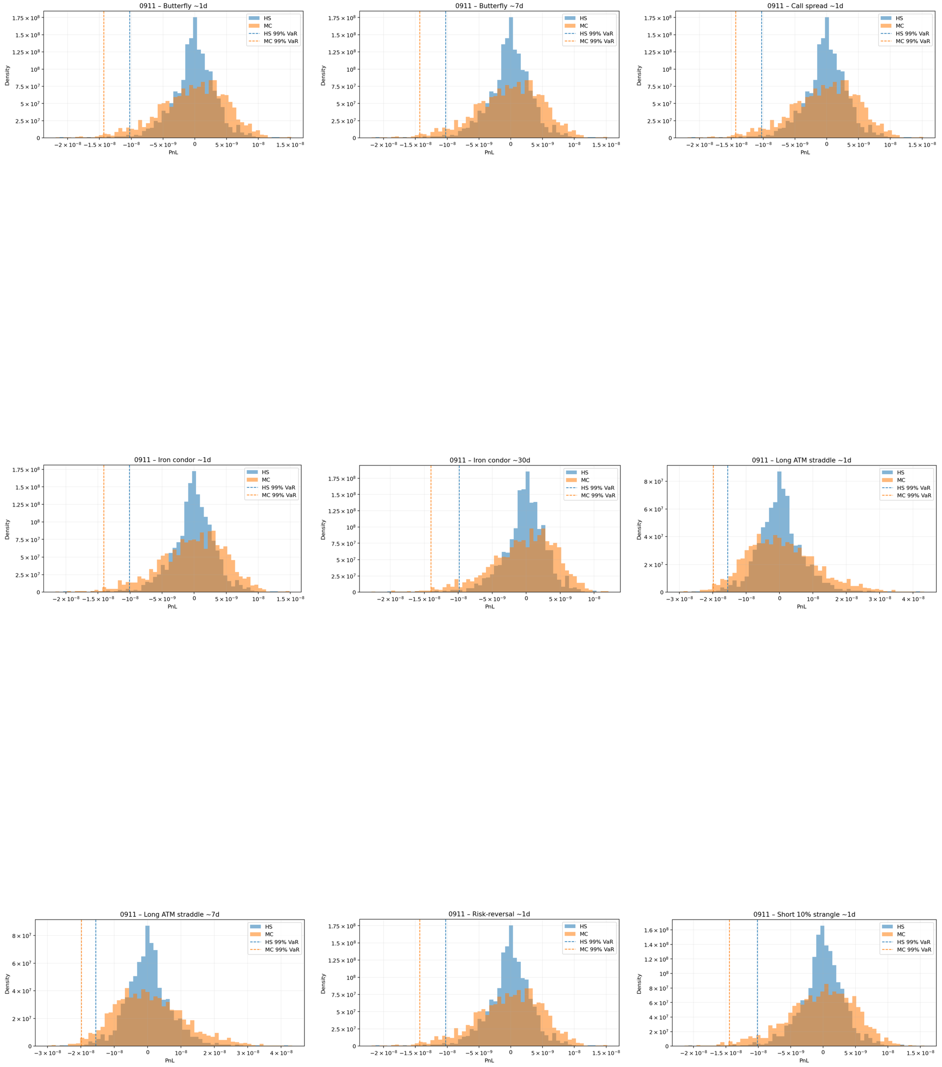
Figure 2. BTCUSD (price of Bitcoin in US dollars) 2025 May 22 price movement.
Risks 14 00151 g002
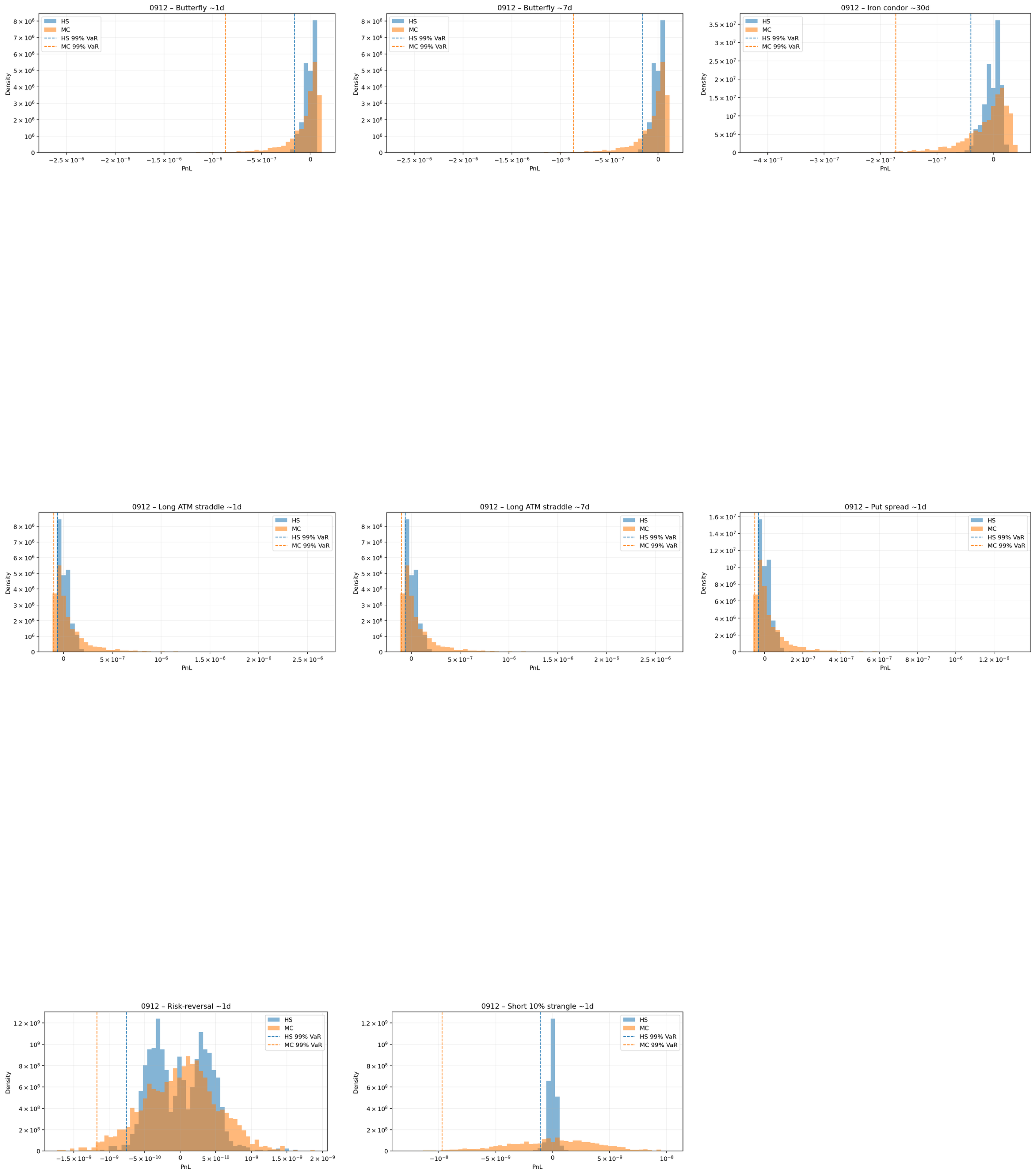
Figure 3. Interval distribution over a week-long period, representing the frequency of different lengths of the time Δ t in seconds between consecutive data points as a histogram (left) and a cumulative distribution function (right).
Risks 14 00151 g003
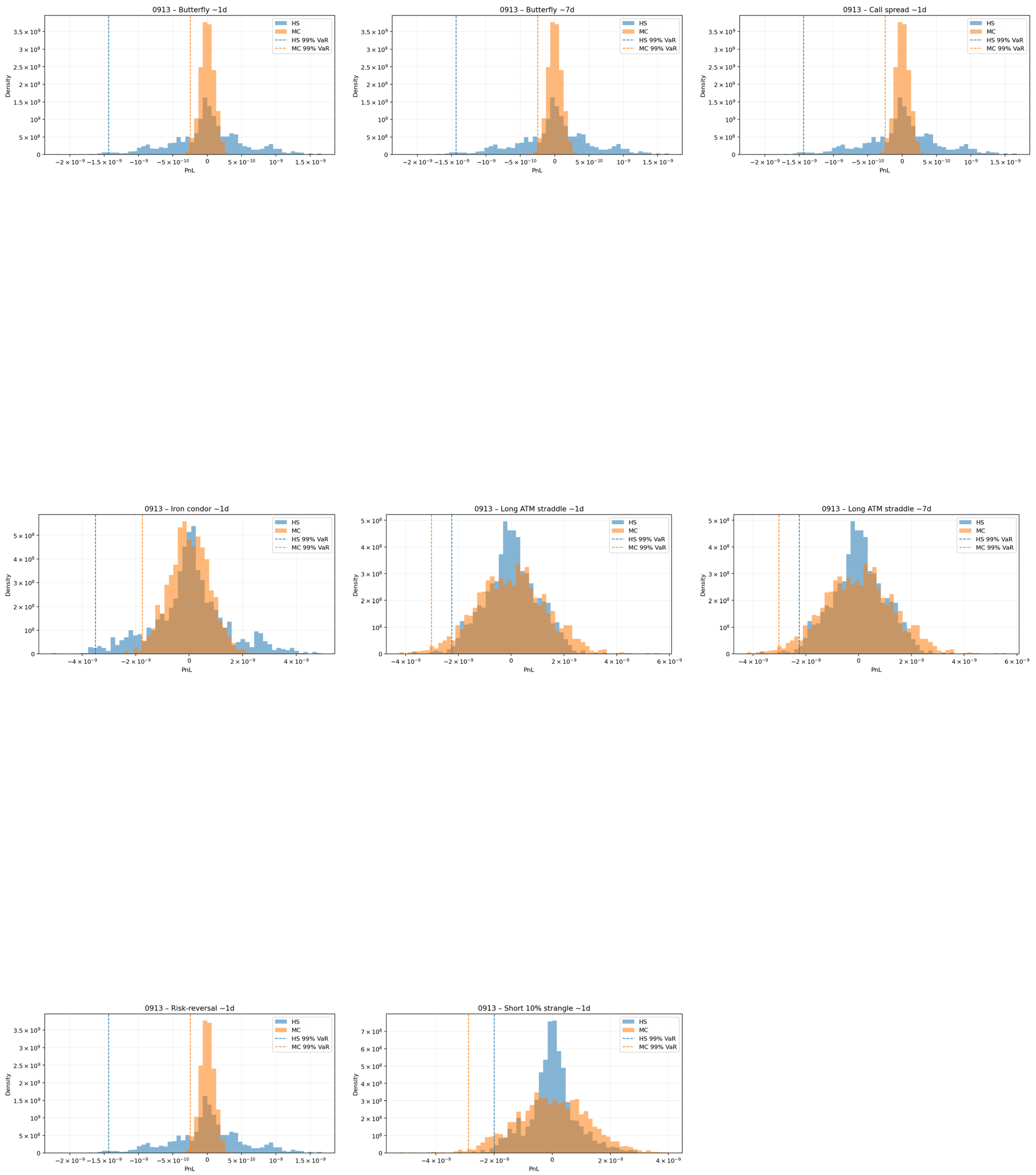
Figure 4. Price evolution of BTCUSD (price of Bitcoin in US dollars) from 7 to 14 September 2025.
Risks 14 00151 g004
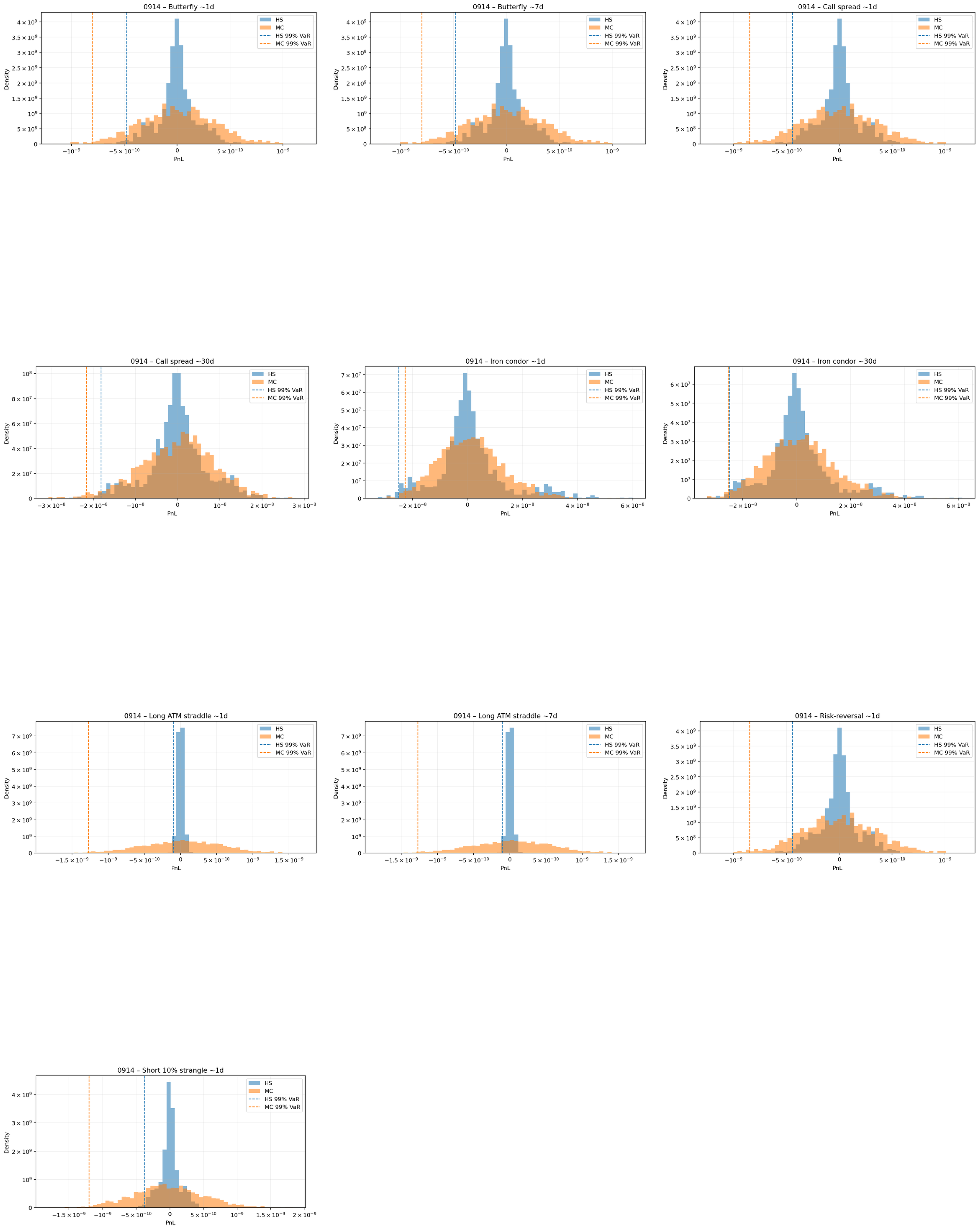
Figure 5. Distribution of observed log-moneyness values per maturity.
Risks 14 00151 g005
Figure 6. Liquid option nodes.
Risks 14 00151 g006
Figure 7. Before and after the arbitrage repair of a surface at an example time step.
Risks 14 00151 g007
Figure 8. Factor decomposition, showing dynamic, statistical, static-arbitrage, and baseline ( G 0 ) factors. (a) Dynamic arbitrage factor. (b) Statistical-accuracy factor. (c) Static-arbitrage factor. (d) G 0 .
Risks 14 00151 g008aRisks 14 00151 g008b
Figure 9. Two factor scores and static no-arbitrage polygon.
Risks 14 00151 g009
Figure 10. Comparison of training curves, representing the total negative log-likelihood (NLL) loss function values at each training epoch with and without drift/diffusion constraints. (a) NLL curve without drift/diffusion constraints. (b) NLL curve with drift/diffusion constraints.
Risks 14 00151 g010
Figure 11. QQ plots of learned neural SDE.
Risks 14 00151 g011
Figure 12. Residual correlation of the learned factors.
Risks 14 00151 g012
Figure 13. Liquid lattice N for the week of 7–14 September 2025, in time to maturity τ (years) against log-moneyness m = ln ( K / S ) . Node density is highest at short maturities and near the money, with the traded moneyness range broadening at longer maturities, in line with the construction of Section 3.2.
Risks 14 00151 g013
Figure 14. Training and test negative log-likelihood over 500 epochs for the week of 7–14 September 2025. The objective converges within ≈130 epochs and plateaus, with a small and stable train/test gap and no subsequent deterioration of the test loss.
Risks 14 00151 g014
Figure 15. Normal quantile–quantile plots of the standardised one-step residuals of the dynamic, statistical and static-arbitrage factors. The central quantiles are approximately linear, while both tails depart from the reference line, indicating symmetric heavy tails (excess kurtosis) relative to the Gaussian assumption of the likelihood.
Risks 14 00151 g015
Figure 16. Pairwise scatter of the factor residuals with Pearson correlations ρ . The dynamic factor is essentially uncorrelated with the other two, while the statistical and static-arbitrage residuals retain a moderate correlation ( ρ = 0.27 ), a mild departure from the diagonal diffusion assumption.
Risks 14 00151 g016
Figure 17. Value-at-Risk (VaR) distributions across option portfolios under neural SDE and historical simulation.
Risks 14 00151 g017
Figure 18. Hedging a 30 day ATM option, compared against Black–Scholes Greek-based methods.
Risks 14 00151 g018
Table 1. Value-at-Risk (VaR) comparison: neural SDE vs. historical simulation.
PortfolioVaR NSDE 99VaR HS 99VaR NSDE 95VaR HS 95Description
Short 10% strangle ∼1 d−0.018899−0.003865−0.013648−0.002575Short 10% OTM call and 10% OTM put, τ 1  d.
Short 10% strangle ∼7 d−0.014940−0.003988−0.010646−0.002645Same short strangle with maturity ∼7d.
Long ATM straddle ∼1 d−0.014211−0.002680−0.013370−0.001680Long ATM call + long ATM put, τ 1  d.
Risk-reversal ±10% ∼1 d−0.006106−0.003822−0.006106−0.002410Long 10% OTM call, short 10% OTM put (directional skew), τ 1  d.
Put spread 5–10% OTM ∼1 d−0.004825−0.002017−0.003476−0.001376Long 10% OTM put, short 5% OTM put; same expiry (debit put spread).
Iron condor 10/20% ∼30 d−0.004094−0.003429−0.003197−0.002309Short 10%/20% OTM call and put wings (short condor), τ 30  d.
Butterfly 10% wings ∼7 d−0.003645−0.002377−0.002677−0.001515Same as above (ATM long body, OTM short wings).
Fly wings = 15% τ = 1 d−0.002920−0.004423−0.001855−0.002849Wider ±15% wing butterfly, 1 d.
Fly wings = 10% τ = 30 d−0.002821−0.004889−0.002049−0.003254±10% wing butterfly, 30 d.
Fly wings = 15% τ = 30 d−0.002810−0.001905−0.001703−0.001362±15% wing butterfly, 30 d.
Iron condor 10/20% ∼1 d−0.002717−0.001909−0.001937−0.001197Short condor with inner 10% and outer 20% strikes, τ 1  d.
Fly wings = 10% τ = 1 d−0.002506−0.004034−0.001470−0.002632±10% wing butterfly, 1 d.
Butterfly 10% wings ∼1 d−0.002506−0.004034−0.001470−0.002632Equivalent short-dated butterfly.
Fly wings = 15% τ = 7 d−0.002457−0.001571−0.002000−0.001165±15% wing butterfly, 7 d.
Calendar ATM 7 d/30 d−0.001962−0.000974−0.001381−0.000652Long 30 d ATM, short 7 d ATM (calendar spread).
Fly wings = 5% τ = 1 d−0.001693−0.003198−0.001181−0.002135Tight ±5% wing butterfly, 1 d.
Call spread ±5% ∼1 d−0.001653−0.002181−0.001653−0.001498Long 5% ITM call, short 5% OTM call; τ 1  d.
Fly wings = 5% τ = 7 d−0.001541−0.003935−0.001112−0.002596±5% wing butterfly, 7 d.
Call spread ±5% ∼30 d−0.001495−0.001580−0.001054−0.0010225% call spread, 30 d.
Fly wings = 5% τ = 30 d−0.001460−0.001538−0.000985−0.000962Tight ±5% wing butterfly, 30 d.
Disclaimer/Publisher’s Note: The statements, opinions and data contained in all publications are solely those of the individual author(s) and contributor(s) and not of MDPI and/or the editor(s). MDPI and/or the editor(s) disclaim responsibility for any injury to people or property resulting from any ideas, methods, instructions or products referred to in the content.