A Framework for Interpreting Machine Learning Models in Bond Default Risk Prediction Using LIME and SHAP

Abstract

Interpretability analysis methods, such as LIME and SHAP, are widely employed to explain the predictions of artificial intelligence models; however, they primarily function as post hoc tools and do not directly quantify the intrinsic interpretability of the models. Although it is commonly assumed that model transparency decreases with increasing complexity, there is currently no standardized framework for evaluating interpretability as an inherent property of AI models. In this study, we examine the prediction of bond defaults using several widely used machine learning algorithms. The classification performance of each algorithm is first evaluated, followed by the application of LIME and SHAP to assess the influence of input features on model outputs. Based on these analyses, we propose a novel approach for quantifying intrinsic model interpretability. The results align with theoretical expectations and provide insights into the trade-off between model complexity and interpretability.

1. Introduction

In recent years, the rapid growth in computational power has fueled significant advances in artificial intelligence (AI) algorithms, including machine learning techniques, which are now widely applied across many fields. In finance, AI-based models have been increasingly adopted for credit risk assessment due to their superior predictive performance and ability to process large and complex datasets. However, despite these advantages, many AI models operate as “black boxes,” raising concerns regarding transparency, interpretability, and regulatory compliance. These concerns have stimulated growing interest in explainable artificial intelligence (XAI), which aims to make model predictions more understandable and trustworthy.

In this study, we investigate the interpretability of machine learning models in the context of corporate bond default risk prediction. Using a sample of bonds issued by Chinese enterprises, we compare traditional statistical models and machine learning methods, including Logistic Regression (LR), Decision Trees (DT), Random Forests (RF), and eXtreme Gradient Boosting (XGBoost). To explain model predictions, we employ two widely used XAI techniques—Local Interpretable Model-agnostic Explanations (LIME) and Shapley Additive Explanations (SHAP). Building on these methods, we propose a novel interpretability metric that evaluates the consistency base on LIME and SHAP as a measure of robustness in model interpretability.

Our empirical analysis yields several important findings. First, although more complex machine learning models such as RF and XGBoost achieve higher predictive accuracy, they exhibit substantially lower interpretability consistency than simpler models. In particular, Logistic Regression demonstrates the highest level of consistency between LIME and SHAP, while XGBoost performs the worst according to the proposed interpretability metric. This result highlights a clear trade-off between predictive accuracy and interpretability robustness across different model classes.

Second, despite differences in model complexity and interpretability, certain financial variables exhibit stable and economically meaningful effects on default risk. Return on assets is consistently associated with a lower probability of default, in line with established financial theory, while the short-term debt-to-total debt ratio plays a significant role in explaining default risk, reflecting firms’ liquidity pressure. These findings suggest that explainable AI techniques can identify core drivers of credit risk, but their reliability depends on both model choice and explanation method.

This study contributes to the literature in several important respects. First, it advances research on explainable artificial intelligence by proposing a quantitative interpretability metric grounded in the consistency between LIME and SHAP, thereby addressing the absence of standardized frameworks for evaluating interpretability (Giudici and Kolesnikov 2026). Second, it enriches the credit risk and corporate bond literature by systematically investigating the trade-off between predictive performance and interpretability in a real-world default prediction context.

The paper is related to several strands of the literature. One strand focuses on the conceptual foundations and logical frameworks of XAI (Miller 2019). Early work by Van Lent et al. (2004) emphasizes interpretable reasoning processes linking inputs, internal representations, and outputs, while Phillips et al. (2021) summarize core principles of XAI, including explanation relevance, user understanding, faithfulness, and confidence. A second strand examines explainable methods for interpreting black-box models, with LIME (Ribeiro et al. 2016) and SHAP (Lundberg and Lee 2017) being among the most widely adopted approaches. A third strand applies XAI techniques across various domains, including asset pricing (Gu et al. 2020; Giudici et al. 2024; LoGrasso 2025), default prediction and credit risk management (Zhang et al. 2025; Nallakaruppan et al. 2024; Lin and Wang 2025; Dichev et al. 2025; Xie and Shingadia 2025; Nkambule et al. 2024; Nayak 2022; Bussmann et al. 2021; de Lange et al. 2022), Cybersecurity (Hermosilla et al. 2025; Jinad et al. 2024), disease prediction (Rezk et al. 2024), public health assessment (Givisis et al. 2025), among others.

The remainder of this paper is organized as follows: Section 2 provides an overview of several machine learning algorithms and their corresponding interpretability measures. Section 3 presents an application analysis using corporate bond data. Section 4 discusses the research methods and presents the conclusions, while Section 5 offers a summary of the paper.

2. Methods

2.1. LIME and SHAP

Local Interpretable Model-Agnostic Explanations (LIME) is a widely used technique for interpreting the predictions of machine learning models. The central idea of LIME is to provide local explanations for individual predictions generated by complex models, thereby enhancing the transparency of the decision-making process without requiring access to the model’s internal structure. As a model-agnostic approach, LIME constructs local surrogate models to approximate the behavior of a black-box model in the neighborhood of a specific instance.

Specifically, LIME operates by perturbing the input features around a given observation to generate a set of synthetic samples. An interpretable and relatively simple model—such as linear regression or a decision tree—is then fitted to these locally generated data, with the objective of approximating the predictions of the original black-box model. The resulting surrogate model provides insights into the relative importance of input features and the factors driving the model’s prediction for that particular instance.

The explanations provided by LIME for each observation x is obtained as follows (Ribeiro et al. 2016):

$$\xi \left(x\right)=\underset{g\in G}{\mathrm{argmin}}\mathcal{L}\left(f,g,{\pi }_x\right)+\Omega (g)$$

(1)

$G$ is a class of potentially interpretable models, g ∈ G is an explanation considered as a model, and f is the model being explained. ${\pi }_x$ is the proximity measure of an instance from x. $\Omega (g)$ is a measure of complexity. Because $\mathcal{L}\left(f,g,{\pi }_x\right)$ is the measure of how unfaithful $g$ is in approximating f in the locality defined by ${\pi }_x$. Then the goal is to minimize $\mathcal{L}\left(f,g,{\pi }_x\right)$ while having $\Omega (g)$ below enough to be interpretable by humans.

LIME is particularly well-suited to scenarios involving highly complex models—such as deep learning architectures and random forests—where the objective is to explain individual predictions in a manner that is understandable to human users. This capability is especially important in application domains such as healthcare, finance, and law, where model interpretability is critical for decision-making and regulatory compliance. In summary, LIME facilitates the interpretation of complex machine learning models by providing human-understandable local approximations that illuminate the reasoning underlying individual predictions.

Shapley Additive Explanations (SHAP) is a widely used approach for interpreting the outputs of machine learning models by assigning a contribution value to each input feature. The method is grounded in Shapley values derived from cooperative game theory, which provide a principled framework for fairly attributing a model’s prediction to its explanatory variables. Importantly, SHAP enables the assessment of each feature’s contribution to an individual prediction in a model-agnostic manner, regardless of the underlying model structure. Conceptually, SHAP treats the machine learning model as a cooperative game in which input features are regarded as players that jointly contribute to the model’s output, interpreted as the reward. The contribution of each feature is quantified by measuring its marginal effect on the difference between the model’s prediction for a given instance and the average prediction across all instances. Formally, the Shapley value for a feature in a model prediction is defined as follows (Lundberg and Lee 2017)

$${\varphi }_i\left(f\right)={\sum }_{S\subseteq N\backslash \{i\}}{\displaystyle \frac{\left|S\right|!(\left|N\right|-\left|S\right|-1)!}{\left|N\right|!}}[f(S\cup \{i\})-f\left(S\right)]$$

(2)

In Equation (2),

${\varphi }_i\left(f\right)$ is the Shapley value for feature $i$.

$S$ represents subsets of features excluding $i$.

$N$ is the set of all features.

$f(S)$ is the model’s prediction for the subset of features $S$.

By analyzing SHAP values, researchers can identify the features that are most influential in driving a model’s predictions. Owing to their solid theoretical foundation, consistency properties, and broad applicability across a wide range of machine learning models, SHAP values have become one of the most widely adopted approaches for model explainability.

2.2. Several Machine Learning Models

We first employ the LIME and SHAP methods to analyze the interpretability of four algorithms used for bond default prediction and then assess the intrinsic interpretability of each model based on the evaluation framework proposed below.

(1) Logistic Regression (LR). Logistic regression is a widely used statistical method for binary classification tasks and can be naturally extended to multi-class classification problems. Its core objective is to model the probability that a given input instance belongs to a particular class. This is achieved through the logistic (sigmoid) function, which maps a linear combination of input features to a value in the interval [0,1], thereby representing the estimated class membership probability.

(2) Decision Tree (DT). Decision trees are supervised machine learning algorithms applicable to both classification and regression tasks. They model decisions and their potential outcomes using a tree-like structure, where nodes represent features or decision points and branches correspond to possible outcomes. The primary objective of a decision tree is to recursively partition the dataset into subsets based on feature values, ultimately yielding predictions for individual instances. Decision trees are highly interpretable and provide an intuitive framework for splitting data according to feature values, which makes them particularly suitable for applications where transparency is important. Nevertheless, decision trees are prone to overfitting, which is why they are often combined with techniques such as pruning or ensemble methods, including Random Forests.

(3) Random Forest (RF). Random Forest is an ensemble learning method widely used for both classification and regression tasks. The algorithm constructs a large number of decision trees during training and generates predictions by aggregating the outputs of individual trees—using the mode for classification and the mean for regression. The primary strength of Random Forest lies in its ability to mitigate overfitting through averaging across multiple decision trees, thereby enhancing both predictive accuracy and generalization performance.

(4) Extreme Gradient Boosting (XGBoost). XGBoost is a widely used and highly efficient machine learning algorithm based on the gradient boosting framework. It has achieved broad adoption due to its speed, predictive accuracy, and strong performance in supervised learning tasks, particularly classification and regression. XGBoost is an ensemble method in which multiple weak learners—typically decision trees—are sequentially combined to form a strong predictive model. The core principle of gradient boosting is to iteratively build models such that each subsequent model aims to correct the errors (residuals) of the previous models.

2.3. Measurement of Interpretability of Machine Learning Models

LIME and SHAP may all have an explanation model that is a linear function of binary variables (Lundberg and Lee 2017):

$$g\left(z^{\prime }\right)={\varphi }_0+{\sum }_{i=1}^M{\varphi }_i{z}_i^{\prime }$$

(3)

In Equation (3), M is the number of simplified input features, $z_i^{\prime }\in {\left\{\mathrm{0,1}\right\}}^M, {\varphi }_i\in R$ is an effect by each feature if $z_i^{\prime }=1$. In SHAP method, ${\varphi }_i$ could be regarded as the Shapley value for feature $i$. On the other hand, in LIME method, ${\varphi }_i$ could be regarded as the contribution of a feature variable in a linear regression model.

Let z = $[z_1^{\prime },z_2^{\prime },\cdots ,z_M^{\prime }]$ is the Shapley value for feature variable, w = $[w_1^{\prime },w_2^{\prime },\cdots ,w_M^{\prime }]$ is the contribution of a feature variable by LIME method, we define the Cosine Similarity of z and w is the measurement of interpretability of AI models (MIAI):

$$MIAI={\displaystyle \frac{z·w}{\parallel z\parallel \parallel w\parallel }}$$

(4)

It is commonly assumed that the interpretability of machine learning models is inversely related to algorithmic complexity. Linear models are generally regarded as the most interpretable, followed by decision trees and related methods, whereas more complex algorithms, such as gradient boosting models (e.g., XGBoost), are often considered less interpretable. Despite this general perception, there is currently no standardized metric or framework for quantitatively assessing model interpretability.

To address this gap, we propose the variable MIAI, defined in Equation (4), as a measure of AI model interpretability. The underlying rationale is that, for a model to be considered interpretable, the feature-level explanations obtained via LIME and SHAP should exhibit a high degree of consistency, particularly regarding the direction and relative importance of feature contributions. Accordingly, we suggest using the correlation between LIME and SHAP results as a quantitative indicator of a model’s interpretability.

The interpretability of an AI model refers to the ease with which the logical relationship between inputs and outputs can be established and understood. Both LIME and SHAP are explanation methods designed to characterize how input features contribute to model predictions, albeit from different methodological perspectives. If different explanation methods exhibit a high degree of consistency in analyzing and reconstructing the input–output relationships, this suggests that the underlying prediction mechanism of the model is more stable and transparent, and therefore easier to interpret. Based on this perspective, this study focuses on measuring the interpretability of AI models and proposes to characterize it through the consistency across different explanation methods.

3. The Interpretability of Machine Learning Models

3.1. Sample Data and Definition of Variables

Sample data for a total of 6471 Chinese corporate bond issuers in 2018 were obtained from the Wind database, among which 50 issuers defaulted in 2019. Based on existing literature, this study selected 16 financial indicators reflecting four key dimensions of bond issuer performance: profitability, operational capacity, solvency, and capital structure (see

Table 1. Definition of variables.

Variable Symbols		Definition of Variables
Identifying variables	Default	if bond default, then default = 1, or default = 0
Feature variables	Prcb	Profit rate of core businesses
	Igrb	Income growth rate of core businesses
	Roa	Return on asset
	Roe	Return on equity
	EBII	EBITDA/Total Income
	Ocebi	Operating cash/EBITDA
	Lr	Liquidity ratio
	Qr	Quick ratio
	Rst	Rate of stock turnover
	Alr	Asset-liability ratio
	Sdtd	Short-term debt/total debt
	Ditc	Debt with interest/total investment capita
	Mtd	Monetary/total debt
	Im	Interest multiples
	Ebit	EBITDA/total debt with interest
	Aou	Audit opinion

), in addition to the external audit opinion. External audit opinions are categorized into four types: (1) unable to express an opinion, (2) unqualified opinion with emphasis of matter paragraph, (3) qualified opinion, and (4) standard unqualified opinion. A numerical value is assigned to each category to indicate the degree to which the financial statements are deemed acceptable, with 1 representing ‘unable to express an opinion,’ 2 for ‘unqualified opinion with emphasis of matter paragraph,’ 3 for ‘qualified opinion,’ and 4 for ‘standard unqualified opinion.

Following common practice in machine learning applications, 80% of the total sample is randomly assigned to the training set, while the remaining 20% is reserved for testing.

3.2. Prediction by Machine Learning Algorithm

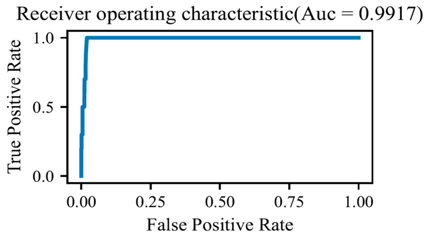
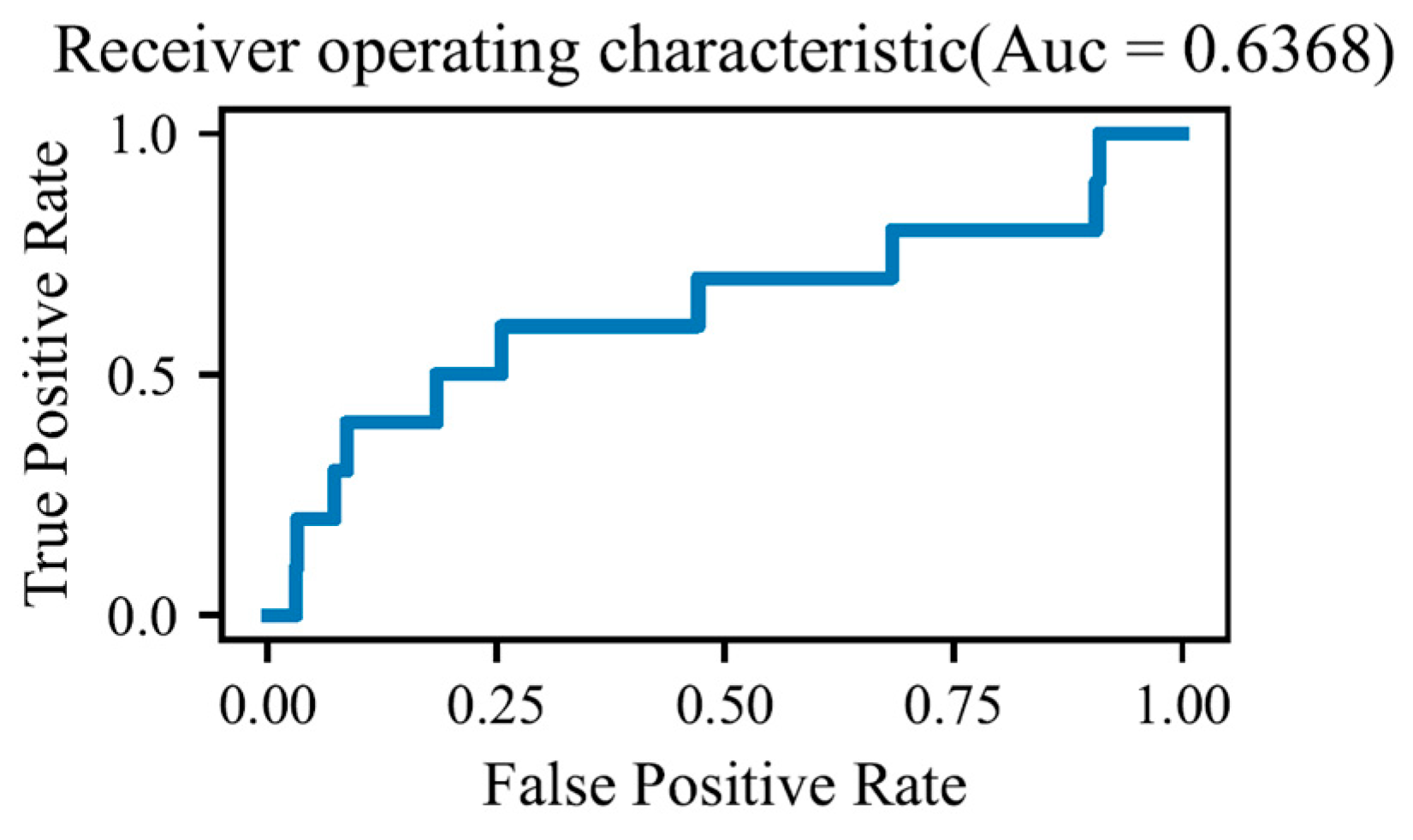
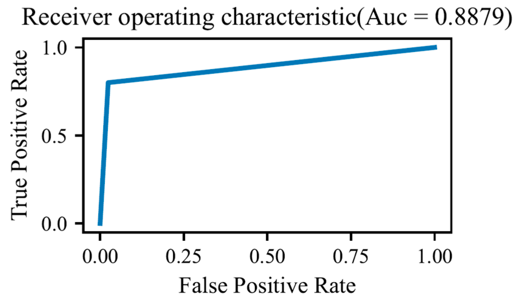
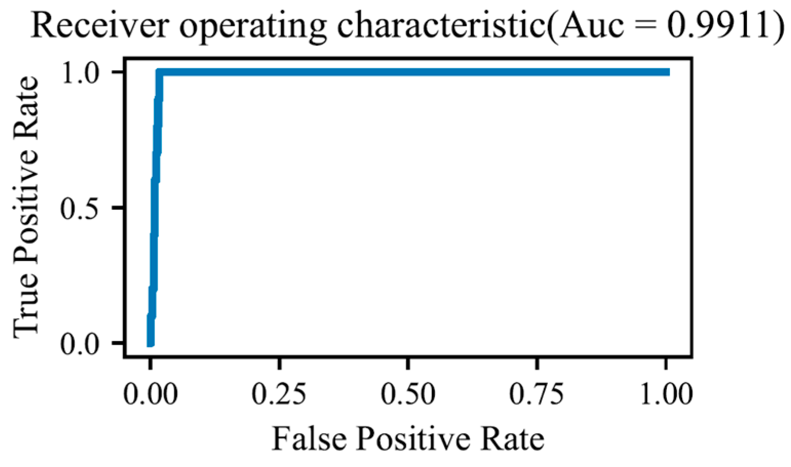
Firstly, using Python’s (3.0 version) machine learning libraries, we trained models for four algorithms: Random Forest (RF), Logistic Regression (LR), Decision Tree (DT), and eXtreme Gradient Boosting (XGBoost), and evaluated their performance on the test dataset. Model performance is assessed using the Area Under the Curve (AUC), a widely adopted metric for evaluating classification models. Figure 1, Figure 2, Figure 3 and Figure 4 show the Auc of four models The performance results for each model are summarized in

Table 2. Comparative prediction of several models.

	LR	DT	RF	XGBoost
AUC	0.6368	0.8879	0.9917	0.9911

.

Due to the presence of class imbalance in the dataset, accuracy is not used as a performance metric. To preserve the integrity of the interpretability analysis, the original imbalanced dataset is retained without applying any data balancing techniques.

Regarding the performance of the predictive models, it is evident that XGBoost and Random Forest outperform Logistic Regression (LR) and Decision Tree (DT) algorithms in terms of classification accuracy. Specifically, the LR model demonstrates the poorest performance on this imbalanced dataset, a result that aligns with common expectations regarding the relative effectiveness of these algorithms under such conditions.

3.3. Measurement of Interpretability Based on LIME and SHAP

On the test dataset, we applied both SHAP and LIME methods to analyze the interpretability of the different models. Since LIME generates explanations at the individual sample level, we used it to evaluate the contribution of each feature to the prediction for each instance. We then computed the average feature contribution across all test samples to obtain an overall assessment of how each feature influences the model’s output. The aggregated results are presented in

Table 3. The impact of features on model output (LIME).

Feature Variables	LR	DT	RF	XGBoost
Prcb	0.0006	−0.0042	−0.00982	−0.0638
Igrb	0.0679	−0.0002	−0.0059	−0.0080
Roa	−0.0111	−0.0155	−0.02057	−0.0402
Roe	−0.0645	0.0125	−0.01548	−0.0070
EBII	0.0015	0.0009	−0.00645	0.0014
Ocebi	0.0013	0.0008	−0.00873	−0.0012
Lr	0.0707	0.0002	−0.00237	0.0184
Qr	0.0445	−0.0036	−0.00337	−0.0007
Rst	0.0274	−0.0011	0.000827	−0.0235
Alr	0.0091	0.0002	−0.00498	0.0259
Sdtd	0.0043	−0.0001	−0.00071	−0.0654
Ditc	−0.0157	−0.0004	−0.01196	−0.0545
Mtd	0.0023	−0.0002	−0.00846	−0.0118
Im	0.0484	0.0001	0.005066	−0.0378
Ebit	0.0763	0.0002	−0.00662	−0.0136
Aou	−0.0189	0.0000	0.0000	−0.1348

.

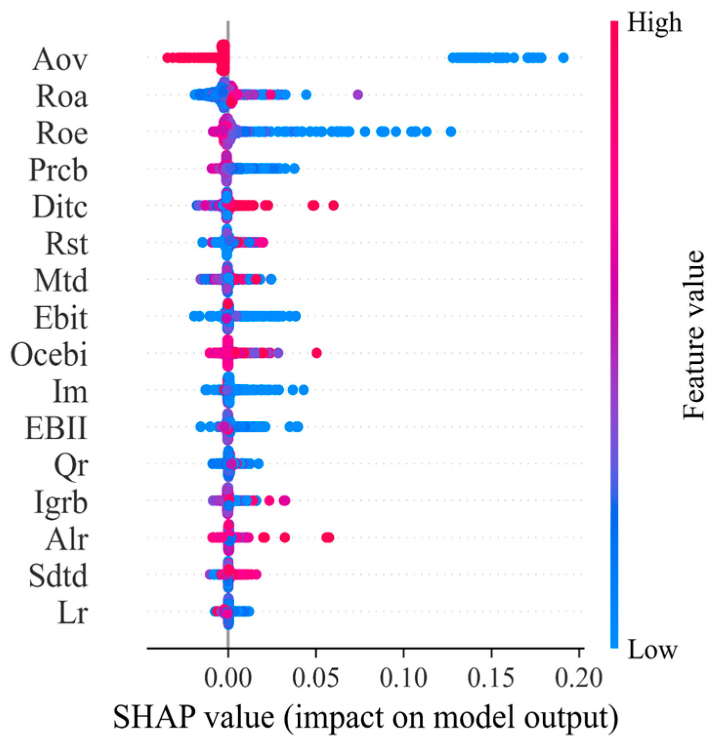
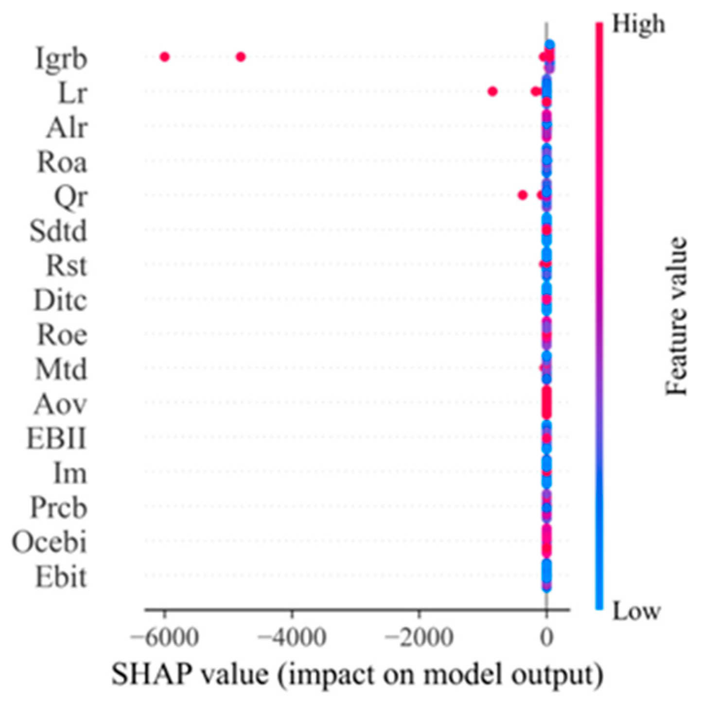
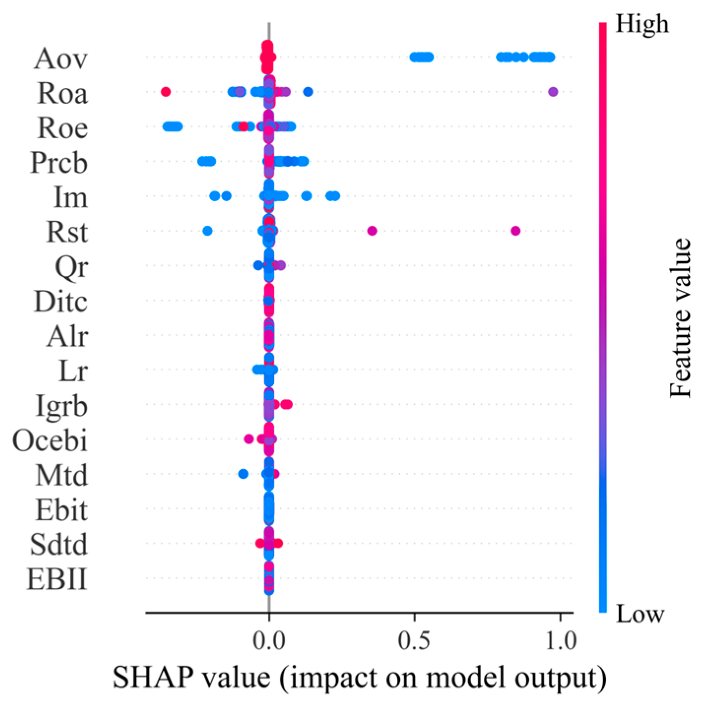
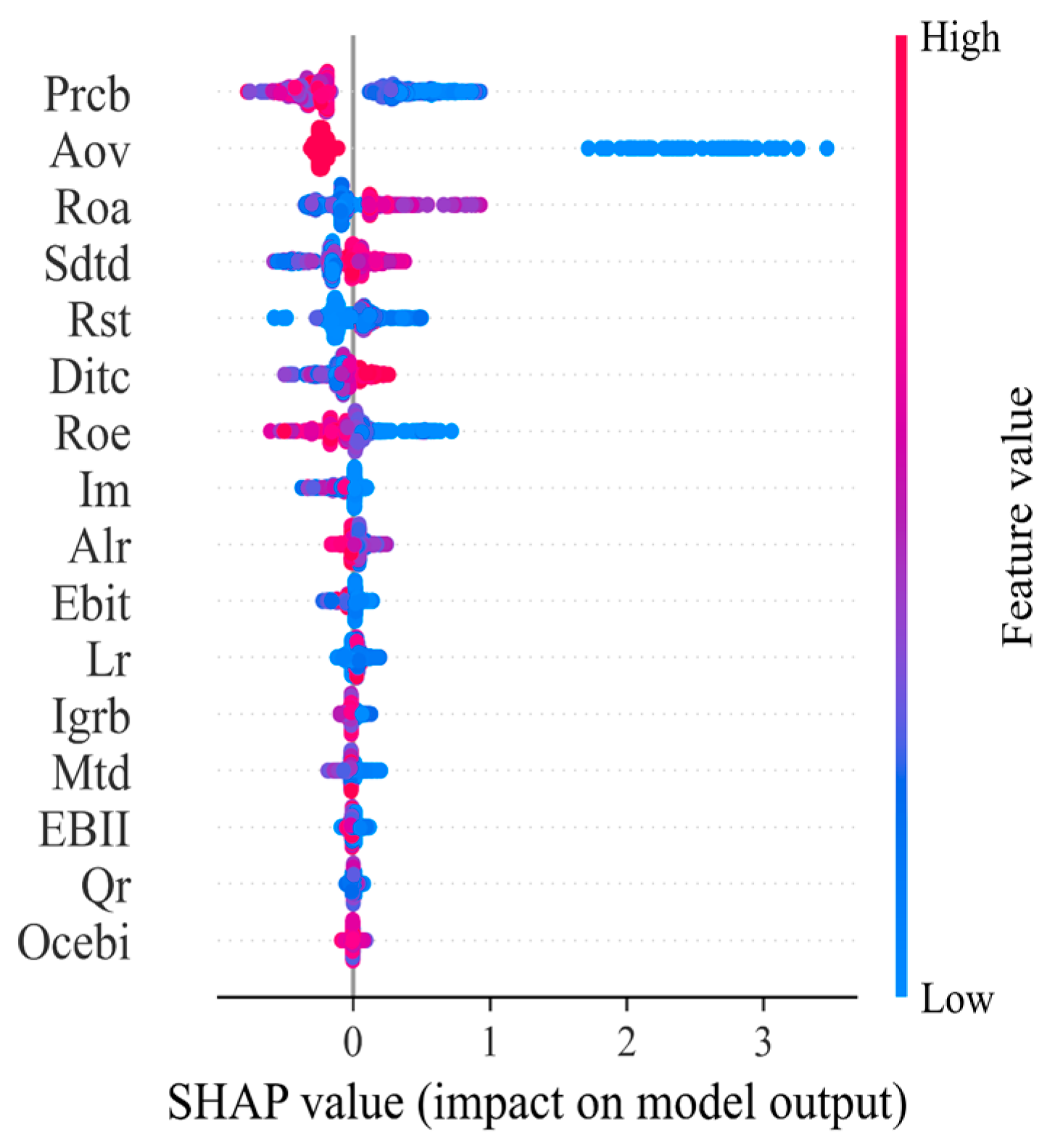
We also calculate the average effect of the SHAP model on each feature value as presented in

Table 4. The impact of features on model output (SHAP).

Feature Variables	LR	DT	RF	XGBoost
Prcb	0.0010	0.0035	0.0006	−0.0116
Igrb	23.4839	0.0011	0.0001	−0.0016
Roa	0.0875	−0.0086	−0.0025	−0.0038
Roe	0.0245	−0.0015	0.0017	−0.0324
EBII	0.0001	−0.0005	0.0004	0.0021
Ocebi	0.0001	0.0023	0.0004	−0.0010
Lr	−3.7279	0.0009	−0.0001	0.0026
Qr	−1.1489	0.0000	0.0005	−0.0007
Rst	−0.2269	0.0004	0.0000	0.0354
Alr	−0.0235	0.0000	0.0005	0.0003
Sdtd	0.1384	0.0001	0.0003	0.0091
Ditc	0.0018	−0.0002	−0.0006	−0.0011
Mtd	0.0123	0.0003	−0.0004	−0.0060
Im	−0.1295	0.0001	0.0007	0.0017
Ebit	0.6573	0.0000	0.0002	0.0003
Aou	−0.0119	0.0267	0.0025	0.0000

.

Figure 5, Figure 6, Figure 7 and Figure 8 show the summary plot. It helps us overview which features are most important for four models.

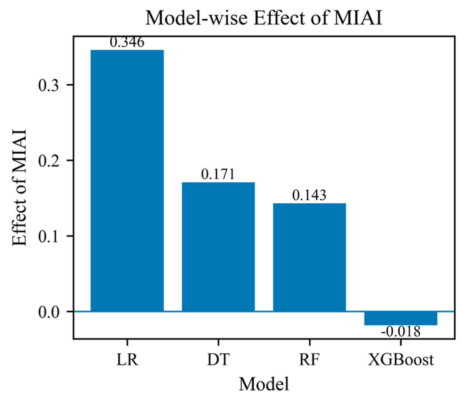
Finally, based on the definition in Equation (4), we computed the correlation between the contributions of each feature, as determined by LIME and SHAP, to assess the interpretability of the four models. The results of this analysis are presented in

Table 5. The measurement of the interpretability of the model.

	LR	DT	RF	XGBoost
$\mathrm{M}\mathrm{I}\mathrm{A}\mathrm{I}$	0.3459	0.1708	0.1430	−0.0182

and Figure 9.

4. Discussion

According to conventional corporate finance theory, ceteris paribus, certain financial indicators are negatively associated with default risk, meaning that higher values of these indicators correspond to a lower likelihood of default. Conversely, the remaining indicators are positively related to default risk, such that larger values are associated with an increased probability of default. For a model to exhibit strong explanatory power, the observed feature contributions should be consistent with these established theoretical relationships.

Beyond the descriptive comparison reported in

Table 6. Comparative analysis with financial theory (LIME).

Feature Variables	The Impact on Default Based on Financial Theory	LR	DT	RF	XGBoost
Prcb	Negative	Positive	Negative	Negative	Negative
Igrb	Negative	Positive	Negative	Negative	Negative
Roa	Negative	Negative	Negative	Negative	Negative
Roe	Negative	Negative	Positive	Negative	Negative
EBII	Negative	Positive	Positive	Negative	Positive
Ocebi	Negative	Positive	Positive	Negative	Negative
Lr	Negative	Positive	Positive	Negative	Positive
Qr	Negative	Positive	Negative	Negative	Negative
Rst	Negative	Positive	Negative	Positive	Negative
Alr	Positive	Positive	Positive	Negative	Positive
Sdtd	Positive	Positive	Negative	Negative	Negative
Ditc	Positive	Negative	Negative	Negative	Negative
Mtd	Negative	Positive	Negative	Negative	Negative
Im	Negative	Positive	Positive	Positive	Negative
Ebit	Negative	Positive	Positive	Negative	Negative
Aou	Negative	Negative	Positive	Positive	Negative

and

Table 7. Comparative analysis with financial theory (SHAP).

Feature Variables	The Impact of on Default Based on Financial Theory	LR	DT	RF	XGBoost
Prcb	Negative	Positive	Positive	Positive	Negative
Igrb	Negative	Positive	Positive	Positive	Negative
Roa	Negative	Positive	Negative	Negative	Negative
Roe	Negative	Positive	Negative	Positive	Negative
EBII	Negative	Positive	Negative	Positive	Positive
Ocebi	Negative	Positive	Positive	Positive	Negative
Lr	Negative	Negative	Positive	Negative	Positive
Qr	Negative	Negative	Positive	Positive	Negative
Rst	Negative	Negative	Positive	Positive	Positive
Alr	Positive	Negative	Positive	Positive	Positive
Sdtd	Positive	Positive	Positive	Positive	Positive
Ditc	Positive	Positive	Negative	Negative	Negative
Mtd	Negative	Positive	Positive	Negative	Negative
Im	Negative	Negative	Positive	Positive	Positive
Ebit	Negative	Positive	Positive	Positive	Positive
Aou	Negative	Negative	Positive	Positive	Positive

, the results provide several important insights into the relationship between model complexity, interpretability, and economic consistency in corporate bond default prediction. Although more complex models such as RF and XGBoost achieve higher predictive performance, their interpretability—measured by the consistency between LIME and SHAP—is substantially lower than that of simpler models. This finding highlights a clear trade-off between predictive accuracy and interpretability, which has been widely discussed in the explainable AI literature.

The higher interpretability score of the logistic regression model suggests that linear models remain advantageous in settings where transparency and stability of explanations are critical, such as financial risk management and regulatory contexts. This result is consistent with prior studies emphasizing that simpler models often produce more stable and economically meaningful explanations, even when their predictive accuracy is relatively limited. In contrast, the lower consistency observed for RF and XGBoost indicates that ensemble-based nonlinear models may generate explanations that are more sensitive to the choice of interpretability method, thereby reducing their reliability for economic interpretation.

Importantly, the feature-level analysis further reveals that certain financial indicators retain robust economic meaning across different models and explanation techniques. For example, return on assets (ROA) exhibits a consistently negative relationship with default risk in the LIME-based analysis, which aligns well with established financial theory and prior empirical evidence that more profitable firms are less likely to default. Similarly, the SHAP-based results show that the short-term debt-to-total debt ratio plays a significant role in default risk assessment, reflecting the well-documented impact of debt maturity structure on firms’ liquidity risk and rollover pressure.

These findings suggest that, even when interpretability consistency is limited at the global level, specific core financial variables may still provide stable and theory-consistent signals of credit risk. From a practical perspective, this implies that explainable AI tools can complement traditional credit risk analysis by identifying economically meaningful drivers of default risk, while caution should be exercised when interpreting explanations from highly complex models. Overall, the results underscore the necessity of jointly considering predictive performance, interpretability robustness, and economic plausibility when applying machine learning models in financial risk assessment.

5. Conclusions

This study proposes a quantitative metric for evaluating the interpretability of explainable artificial intelligence (XAI) models. Specifically, we suggest assessing model interpretability by integrating LIME and SHAP methods. Using our dataset, we applied this approach to four commonly used classification algorithms, and the resulting interpretability assessments are consistent with intuitive expectations.

Given that the interpretability of AI models remains an area of ongoing debate, the proposed method may have certain limitations. For example, since the underlying LIME and SHAP methods are not fully robust across all data environments, applying our approach to different datasets may yield varying conclusions. Nonetheless, we consider the proposed method a meaningful contribution toward addressing this challenge. Future research could extend this framework by integrating additional post hoc interpretability techniques to further refine and enhance the assessment of model interpretability.

The most important limitation of this study is the theoretical justification for the proposed interpretability metric. Specifically, our approach assumes that a high correlation between LIME- and SHAP-based feature explanations reflects greater model interpretability. While this assumption is supported by empirical observations in our dataset, the underlying theoretical or causal rationale linking explanation consistency to model interpretability remains to be fully established. Future research could aim to develop formal theoretical frameworks or axiomatic definitions that rigorously connect explanation agreement with interpretability, potentially integrating human judgment or expert evaluation to validate quantitative metrics.