Financial Mechanisms of Corporate Bankruptcy: Are They Different or Similar Across Crises?

Abstract

One primary objective of the early warning system literature is to construct more accurate financial vulnerability prediction models and investigate the mechanisms and key factors that differentiate healthy from vulnerable financial states. Despite the importance of identifying and predicting financial vulnerabilities, existing research does not fully explain whether—and how—the financial behavior associated with corporate bankruptcy differs across crises. This study investigates (1) whether the financial mechanisms of corporate bankruptcy differ across three crises—the Global Financial Crisis, the European debt crisis, and the COVID-19 crisis; (2) whether these crises differ from tranquil periods before the Global Financial Crisis and after the European debt crisis; and (3) how these differences manifest. To conduct this analysis, we introduce a unique framework based on a random forest model, utilizing a corporate bankruptcy dataset spanning 2002–2023. The results show that the bankruptcy mechanisms during the Global Financial Crisis and the European debt crisis are not significantly different, whereas the COVID-19 crisis exhibits distinct characteristics. Additionally, we find that “Credit period days,” “Collection period days,” “Gross margin,” and “Solvency ratio (asset-based)” are key financial factors distinguishing these events.

1. Introduction

Since the late 2000s, the world has experienced three major economic crises that have severely impacted economies and societies: the Global Financial Crisis (2007–2009, hereafter Glob.C), the European debt crisis (2010–2012, hereafter EU.C), and the COVID-19 crisis (late 2019–present, hereafter COV.C). These devastating events have intensified research on identifying and predicting vulnerabilities across sectors, including firms (Jayasekera 2018; Tanaka et al. 2019), financial institutions (Berger and Bouwman 2013; Demirguc-Kunt et al. 2013; Drehmann and Tarashev 2013; Frankel and Saravelos 2012; Tanaka et al. 2016, 2018; Rose and Spiegel 2011; Vazquez and Federico 2015; Beutel et al. 2019; Kristóf and Virág 2022; Frankel and Rose 1996; Ward 2017; Silva et al. 2017; Acharya et al. 2017), and national or currency crises (Joy et al. 2017; Frankel and Rose 1996; Frankel and Saravelos 2012; Frankel and Wei 2004; Bitetto et al. 2023; Ghosh and Ghosh 2002).

Since the Global Financial Crisis of 2007–2009, the development of reliable and accurate early warning systems (EWS) has attracted significant attention from stakeholders seeking early indicators of systemic financial crises from both macroeconomic and microeconomic perspectives (Claessens and Horen 2015; Frankel and Saravelos 2012; Tola and Waelti 2018). This focus stems from the fact that bank failures can destabilize entire financial systems and cause long-term damage to national and global economies (Berger and Bouwman 2013; Demirguc-Kunt et al. 2013; Drehmann and Tarashev 2013; Frankel and Saravelos 2012; Tanaka et al. 2016, 2018; Rose and Spiegel 2011; Vazquez and Federico 2015).

The importance of EWS in detecting financial risk at the corporate level has also gained recognition, as corporate failures due to financial instability can affect subsidiaries, employees, clients, and lenders, potentially causing substantial economic damage (Chakraborty and Sharma 2007; Jayasekera 2018; Stewart et al. 2017; Tanaka et al. 2019; Campbell et al. 2008; Barboza et al. 2017; Altman et al. 2017; Altman 1993, 1984; Altman et al. 1994; Tian and Yu 2017). Because corporate activity is a fundamental pillar of industrial and economic development, assessing firms’ financial stability is crucial for gauging overall economic health. Moreover, analyzing corporate vulnerability provides valuable insights for a range of stakeholders—including governments, fund managers, financial institutions, and regulators—enabling them to anticipate economic trends and implement measures to prevent serious and sometimes irreversible losses.

Despite their varied applications, early warning systems share a common mechanism: assessing the likelihood of transitions from stable to unstable conditions (e.g., bankruptcy, stock-price crashes, or currency collapses). A primary objective of EWS research is therefore to develop more accurate models for predicting financial vulnerability; another is to identify and analyze the financial indicators that differentiate stable from unstable states. However, while EWS are valuable tools for identifying and predicting financial vulnerability, they do not clarify whether—and how—financial vulnerabilities differ across crises. Notably, most existing studies focus on financial institutions and their macroeconomic consequences, whereas investigations into corporate financial behavior during crises remain limited.

This study contributes to the literature on economic crises by examining whether the financial behavior associated with corporate bankruptcy differs across three crises, using only the fiscal data of bankrupt firms. Specifically, we propose a simple, reproducible machine learning framework that uses solely the fiscal data of bankrupt firms to build a random forest model (Breiman 2001) and investigate whether—and how—the mechanisms of bankruptcy differ across the Glob.C, EU.C, and COV.C periods. To the best of our knowledge, this is the first study to explore the differences in financial mechanisms among these three crises—and between crisis and tranquil periods—using only data from bankrupt firms.

Intuitively, if the financial factors contributing to bankruptcy differ across crises, this should be reflected in model accuracy, as it implies the presence of distinguishable patterns that the model can detect. Hence, higher accuracy indicates greater differences in the mechanisms of bankruptcy across crises, suggesting that the causes of bankruptcy are crisis-specific.

Focusing exclusively on bankrupt firms yields valuable insights, enabling us to identify how bankruptcy processes and their key drivers differ across crises. For example, the Global Financial Crisis stemmed from the collapse of the U.S. housing market, which severely disrupted global financial markets and banking systems. The ensuing Great Recession weakened European economies, giving rise to sovereign-debt problems and institutional failures. By contrast, the COVID-19 crisis was precipitated by pandemic lockdowns that abruptly halted global economic activity and induced a sharp contraction and deep recessions. Our random forest framework helps determine whether—and how—corporate bankruptcy mechanisms vary across these crises. Such distinctions cannot be recovered from conventional binary classification studies that simply compare bankrupt with nonbankrupt firms, because these approaches only reveal the differences in financial behavior between healthy and distressed firms within a given crisis. Moreover, the nonlinear random forest approach is critical for detecting more intricate financial mechanisms that differentiate bankruptcy risk.

In practice, while the Chicago Board Options Exchange’s Volatility Index (VIX) is often cited as a “fear index,” our framework offers a more granular, mechanism-based approach to assessing risk. It may thus prove useful in managing crisis-specific risk factors or constructing financial risk indices. For instance, a sudden increase in model accuracy could signal a structural change or the emergence of a new crisis.

The objective of this study is not to conduct a predictive “horse race” between machine learning models or to search for new indicators to improve EWS accuracy. Instead, we focus on simplicity and reproducibility: we use only financial ratios and apply a simple yet effective random forest algorithm, whose hyperparameters are easier to tune than those of SVMs or deep-learning models (Tanaka et al. 2016, 2018, 2019).

The experimental results show no significant financial differences between bankruptcies during the Glob.C and EU.C, whereas COV.C exhibits a distinct mechanism. Interestingly, our findings also suggest that bankruptcies from the pre-Glob.C to post-EU.C periods—including both crisis and tranquil phases—share similar characteristics. By contrast, bankruptcies during the COV.C display unique patterns.

Surprisingly, the key variables that distinguish crises and tranquil periods are largely consistent: “Credit period days,” “Gross margin,” “Collection period days,” and “Solvency ratio (asset-based).” All models identify “Credit period days” and “Collection period days” as particularly important, suggesting that these two variables alone may strongly influence model accuracy.

The remainder of this paper is organized as follows. Section 2 reviews the literature on early warning systems. Section 3 outlines our methodology. Section 4 presents the empirical analysis of whether—and how—the financial behavior of bankrupt firms differs across the three crises and relative to tranquil periods. Section 5 concludes and suggests directions for future research.

2. Literature Review of Early Warning Systems

The development of financial vulnerability and bankruptcy models for financial institutions and companies has long been a major topic of interest. In particular, early warning systems (EWS) that detect financial risks and vulnerabilities gained prominence after the Global Financial Crisis and the Eurozone crisis (Oet et al. 2013; Rose and Spiegel 2011; Frankel and Saravelos 2010, 2012; Cleary and Hebb 2016), prompting the creation of various methods to assess the financial fragility of both institutions and firms. Analyses of institutional and corporate vulnerabilities are essential to economic stability: the former provide financial intermediation and support, while the latter serve as the engine of the economy.

Earlier approaches to vulnerability analysis primarily used discriminant analysis, multivariate logistic regression, and probit models to predict crises at financial institutions (Drehmann and Juselius 2014; Demirguc-Kunt et al. 2013; Oet et al. 2013; Martin 1977; Bussiere and Fratzscher 2006; Brownlees and Engle 2016) and with corporate bankruptcy (Brédart 2014; Hillegeist et al. 2004; Lennox 1999; Ohlson 1980; Campbell et al. 2008; Altman 1968; Beaver 1966). Multivariate linear modeling is a convenient and widely used framework for interpreting the impact of explanatory variables, especially in economics.

Following the Global Financial Crisis, numerous studies investigated financial risk in institutions—particularly corporate governance and risk management (Silva et al. 2017; Tola and Waelti 2018)—because financial institutions were at the epicenter of the crisis and sustained substantial damage worldwide. Nevertheless, assessing corporate-level financial vulnerability remains equally critical. Corporate bankruptcies can cause severe economic losses through both direct effects (e.g., job and income loss for employees, unpaid loans for creditors) and indirect effects (e.g., reduced tax revenues for governments).

The modeling of corporate financial vulnerability has a long history, dating back to Altman (1968) and Beaver (1966). Analyzing corporate bankruptcy benefits from data richness, as the number of companies far exceeds that of financial institutions, providing a broader range of bankruptcy cases. Altman, for instance, developed Z-scores using discriminant analysis based on financial statements, incorporating business ratios such as working capital, retained earnings, EBIT, sales-to-assets, and the market value of equity to book value of liabilities (Altman 1968; Altman et al. 2017). He further extended his work using statistical models, including neural networks and linear discriminant analysis (Altman 1984, 1993; Altman et al. 1994).

Shumway (2001) and Chava and Jarrow (2004) introduced dynamic or survival models for evaluating bankruptcy risk. Their key insight was that bankruptcies often result not from a single shock but from the gradual accumulation of financial stress over time. These models leverage time-series data to capture the temporal dynamics of financial vulnerability.

More recently, the literature on financial vulnerability analysis has shifted towards machine learning as an alternative, data-driven approach (Alpaydin 2014; Geron 2022). This trend applies to both institutional and corporate vulnerability research (Jayasekera 2018; Tanaka et al. 2019; Stewart et al. 2017; Chakraborty and Sharma 2007; Tanaka et al. 2016, 2018; Barboza et al. 2017; Liu et al. 2023; Holopainen and Sarlin 2017), as business and economics researchers increasingly engage with large-scale data analysis (Varian 2014; Einav and Levin 2014). A substantial body of the EWS literature follows this trend, with machine learning approaches often reported to produce more accurate, reliable, and systematic models than the conventional multivariate logistic and probit models long used in economics (Brédart 2014; Drehmann and Juselius 2014; Hillegeist et al. 2004; Lennox 1999; Ohlson 1980; Beaver 1966; Altman 1968; Martin 1977).

As an alternative to linear models, decision trees (Breiman et al. 1984) have been widely applied to predict and analyze financial vulnerabilities and corporate bankruptcies (Kim et al. 2008; Messier and Hansen 1988; Shirata 2003), as well as bank failures (Kristóf and Virág 2022). Decision trees adopt a nonlinear, inductive approach, creating decision boundaries for failure via a sequence of splitting rules that partition the space of explanatory variables. Shirata (2003) developed a bankruptcy model by analyzing financial data from 1426 bankrupt and 3434 nonbankrupt companies. He built a linear model using variables extracted from decision trees—such as retained earnings to total assets, inventory-turnover period, interest expenses to sales, and net income before tax to total assets—and showed that this model outperformed conventional logistic models (Altman 1968; Ohlson 1980; Lennox 1999) in discriminatory power. Kim et al. (2008) likewise emphasized the importance of nonlinear models, including decision trees and neural networks, for decision-making in bankruptcy prediction, comparing their performance with linear models using data from 30 bankrupt and 30 nonbankrupt companies.

Machine learning approaches have also been increasingly applied to institutional vulnerability analysis. Kristóf and Virág (2022) examined the predictive accuracy of C5.0 decision-tree and neural-network models in assessing failure risk among EU-27 banks, finding that such models outperform traditional logit approaches. Climent et al. (2019) implemented an extreme gradient boosting (XGBoost) model to predict bank failures in the Eurozone, using 25 annual financial ratios as early warning predictors.

Tanaka et al. developed predictive models for both corporate (Tanaka et al. 2019) and banking-sector (Tanaka et al. 2016, 2018) vulnerabilities using random forest algorithms. They introduced a methodology for measuring and analyzing industry- and country-specific vulnerabilities by aggregating the potential risks associated with corporate liabilities and job losses, based on predicted bankruptcy probabilities using micro-level firm data from various countries. Furthermore, they created financial hazard maps to evaluate national-level vulnerability in terms of expected asset losses and bank-failure probabilities. Vulnerability assessments of industrial and financial sectors are crucial for crisis detection, given that corporate economic and technological activity forms the foundation of macroeconomic stability. These authors argued that prediction accuracy is essential for reliable risk evaluation, reinforcing the value of machine learning approaches.

However, much of the current EWS literature still focuses primarily on developing accurate models to detect transitions from stable to distressed financial conditions—such as bankruptcies of firms or financial institutions—and on identifying factors that distinguish between these states. Moreover, while much of the crisis literature emphasizes the financial stability of institutions, relatively few studies have examined corporate financial behavior during times of crisis.

To address this gap, the present study focuses on corporate bankruptcies and investigates (1) whether bankruptcy mechanisms differ across the three most recent global crises, (2) whether they differ from those observed during tranquil periods, and (3) which financial indicators best distinguish between these scenarios.

3. Methodology of Bankruptcy Analysis

We propose a novel machine learning framework for evaluating economic crises through the following steps:

• We analyze whether the financial behavior associated with corporate bankruptcy differs across the three crises by employing random forest models. Specifically, we construct three binary classification models to distinguish between the following crisis pairs: Glob.C vs. EU.C, Glob.C vs. COV.C, and EU.C vs. COV.C. Intuitively, if the financial factors contributing to bankruptcy during two different crises are distinct, this should be reflected in model accuracy, as it implies that the random forest model can detect identifiable differences in the data. Therefore, higher model accuracy would indicate greater differences in the financial factors or mechanisms of bankruptcy between crises, suggesting that these bankruptcies occurred for different reasons.
• We conduct a similar analysis to examine how the financial behavior of bankrupt firms during crises differs from that during tranquil periods. We define two tranquil periods: pre-Glob.C (2002–2006, hereafter preGlob.Trq) and post-EU.C (2013–2018, hereafter postEU.Trq). For each crisis, we build two models (crisis vs. each tranquil period), resulting in a total of six models.
• We analyze the important variables identified by each random forest model to assess the differences in financial indicators that contribute to bankruptcy across periods.
• We further investigate the top three most important variables in each model using partial dependence analysis—a technique that helps interpret machine learning models by providing detailed insights into the marginal effect of individual predictors on the outcome.

3.1. Data

The data used in this experiment were collected from Orbis, which provides comprehensive coverage of company information across countries in standardized data formats. Evaluating bankruptcy based on such widely available data enables researchers, investors, and practitioners to improve their financial and economic risk management, thereby reducing credit risk and financial vulnerability across industries.1

We obtained financial statements for industrial companies operating in member countries of the Organisation for Economic Co-operation and Development (OECD) (hereafter referred to as “OECD companies”) as recorded in Orbis. The following search criteria were applied to filter the companies:

• Status: Bankruptcy or Dissolved (due to bankruptcy).
• Size classification: Large, Very large.
• Entity type: Corporate.
• Consolidation code:

  ➢

  C1 (consolidated accounts with no unconsolidated companion).

  ➢

  C2 (consolidated accounts with an unconsolidated companion).

  ➢

  U1 (unconsolidated accounts with no consolidated companion).

  ➢

  U2 (unconsolidated accounts with a consolidated companion).

• World region/Country/Region in country: OECD.

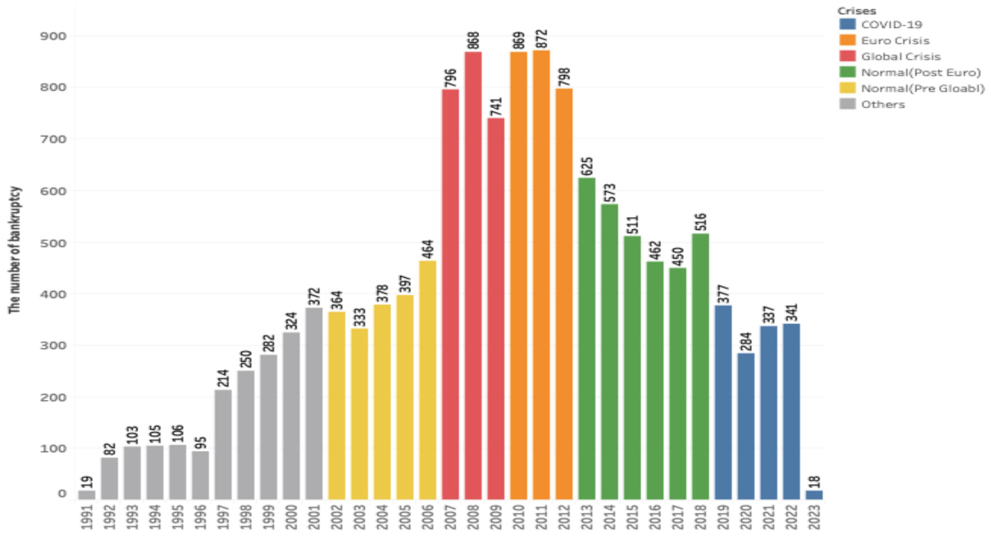
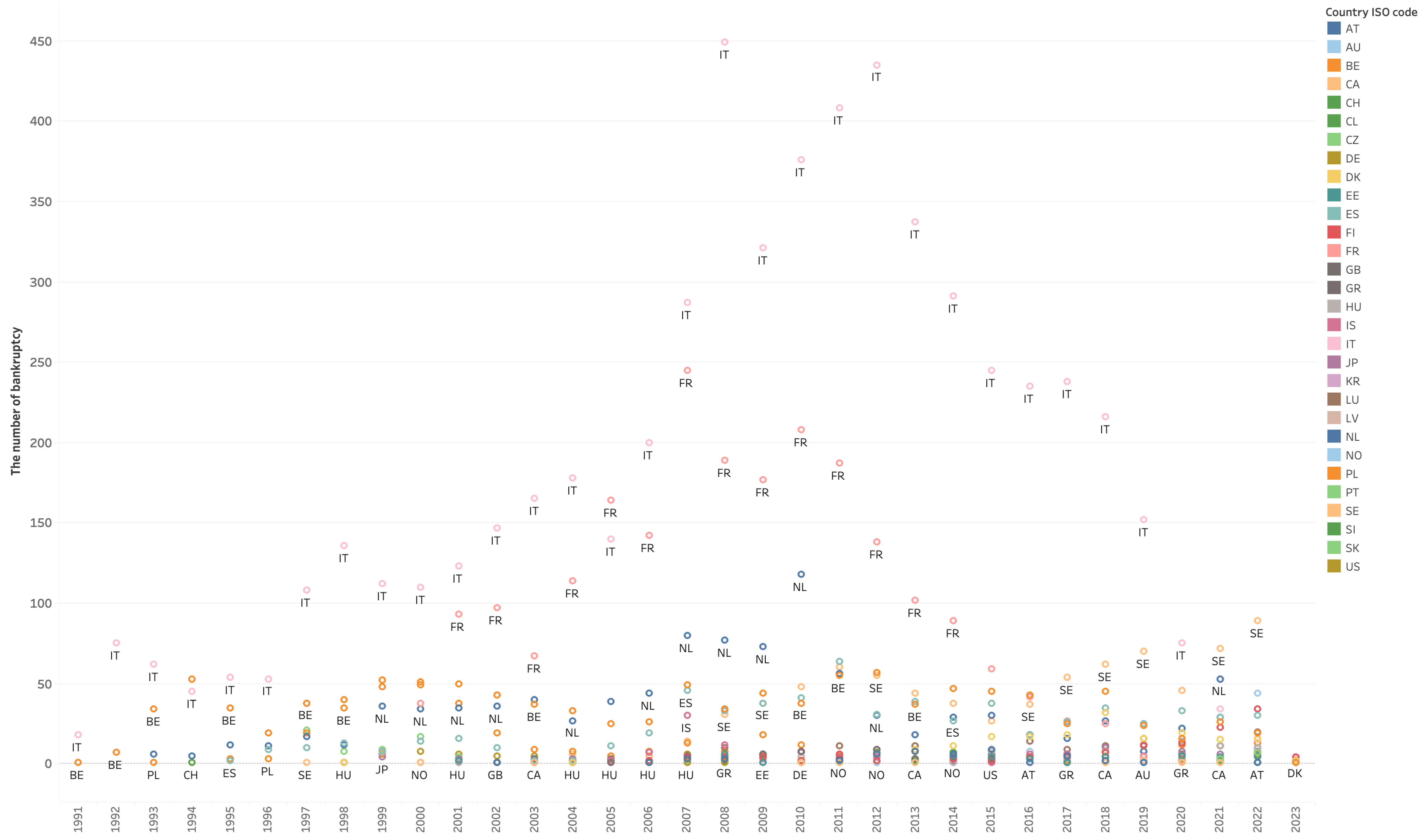
We collected annual Global Ratio data, which are categorized into three groups—profitability, operational, and structural ratios—comprising 26 indicators in total (13, 7, and 6 variables, respectively). Figure A1 and Figure A2 in Appendix A show the number of bankrupt companies by year and by OECD country in the Orbis database.

3.2. Modeling

3.2.1. Definition of Crisis Events

We analyze the differences in three recent economic crises: the Global Financial Crisis, the European debt crisis, and the COVID-19 crisis. These crises are defined as follows:

• Global Financial Crisis (Glob.C), 2007–2009: The collapse of the U.S. housing market bubble caused a multinational financial crisis spillover due to the interconnectedness of the global financial system. This crisis caused extreme damage to global financial markets and banking systems. This was one of the worst recessions in recent decades. It is also said to be the worst economic crisis since the 1929 Wall Street crash.
• European debt crisis (EU.C), 2010–2012: The Great Recession of the Glob.C weakened the economies of European Union countries and created a foreign capital cash flow problem for countries dependent on foreign lending, exposing vulnerabilities in the Eurozone’s structure. Hence, the EU.C was caused by worsening the countries that had substantial current account deficits and triggered high government debt and institutional failures.
• The COVID-19 crisis (COV.C), 2019–2023: While the Glob.C and EU.C are economic crises that occurred in the financial system, the COV.C is an economic crisis triggered by the pandemic. During the early stage of the COVID pandemic, a large portion of the world was under some form of lockdown, which caused serious damage to the stock market and global supply chain. This incident literally stopped the global economy and led to a sharp contraction in economic activity, triggering a deep economic recession. To obtain a reasonable amount of data, for this research, the COV.C period was set as 2019 to 2023. It is also considered to be one of the worst recessions in recent decades.

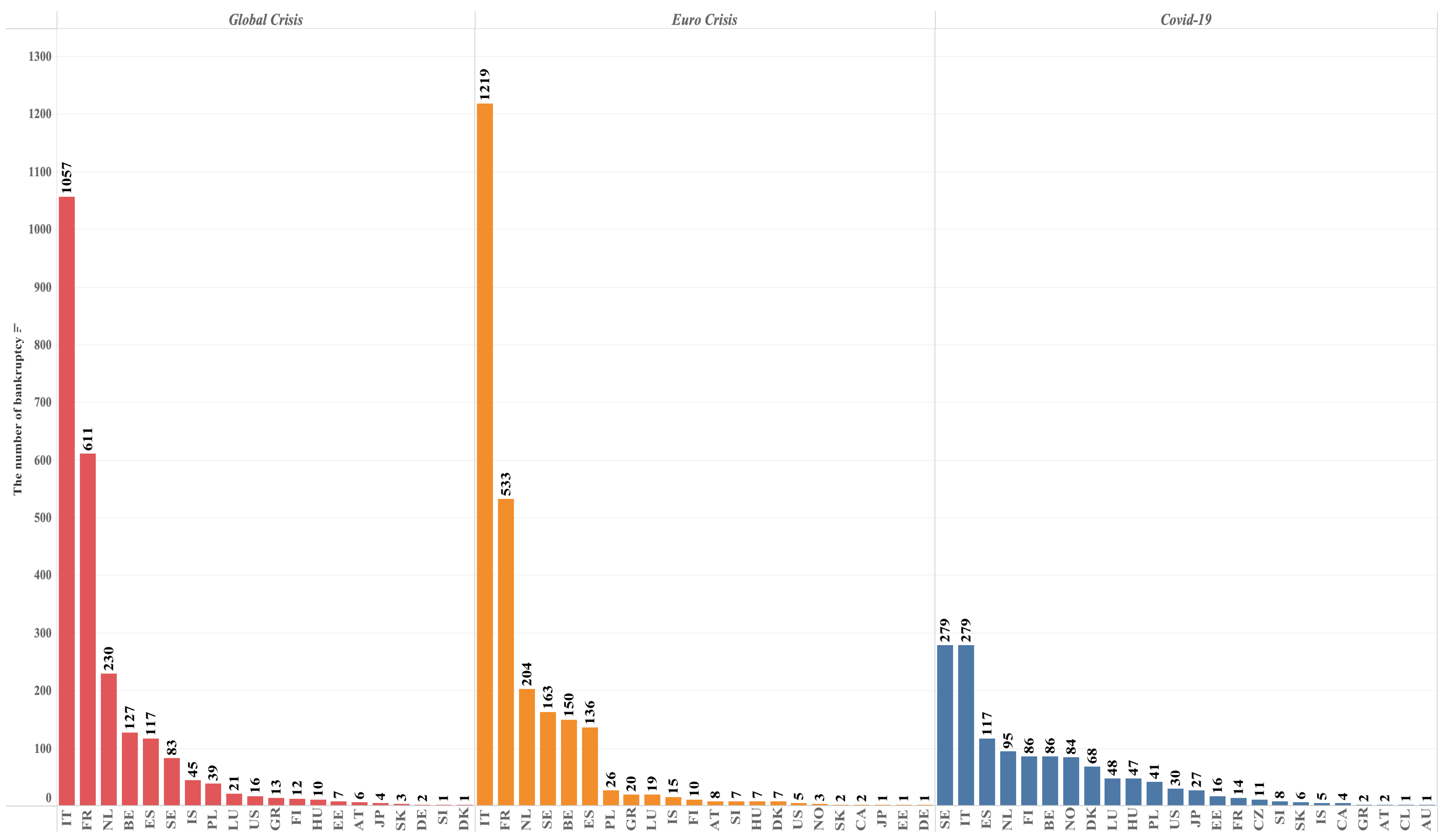
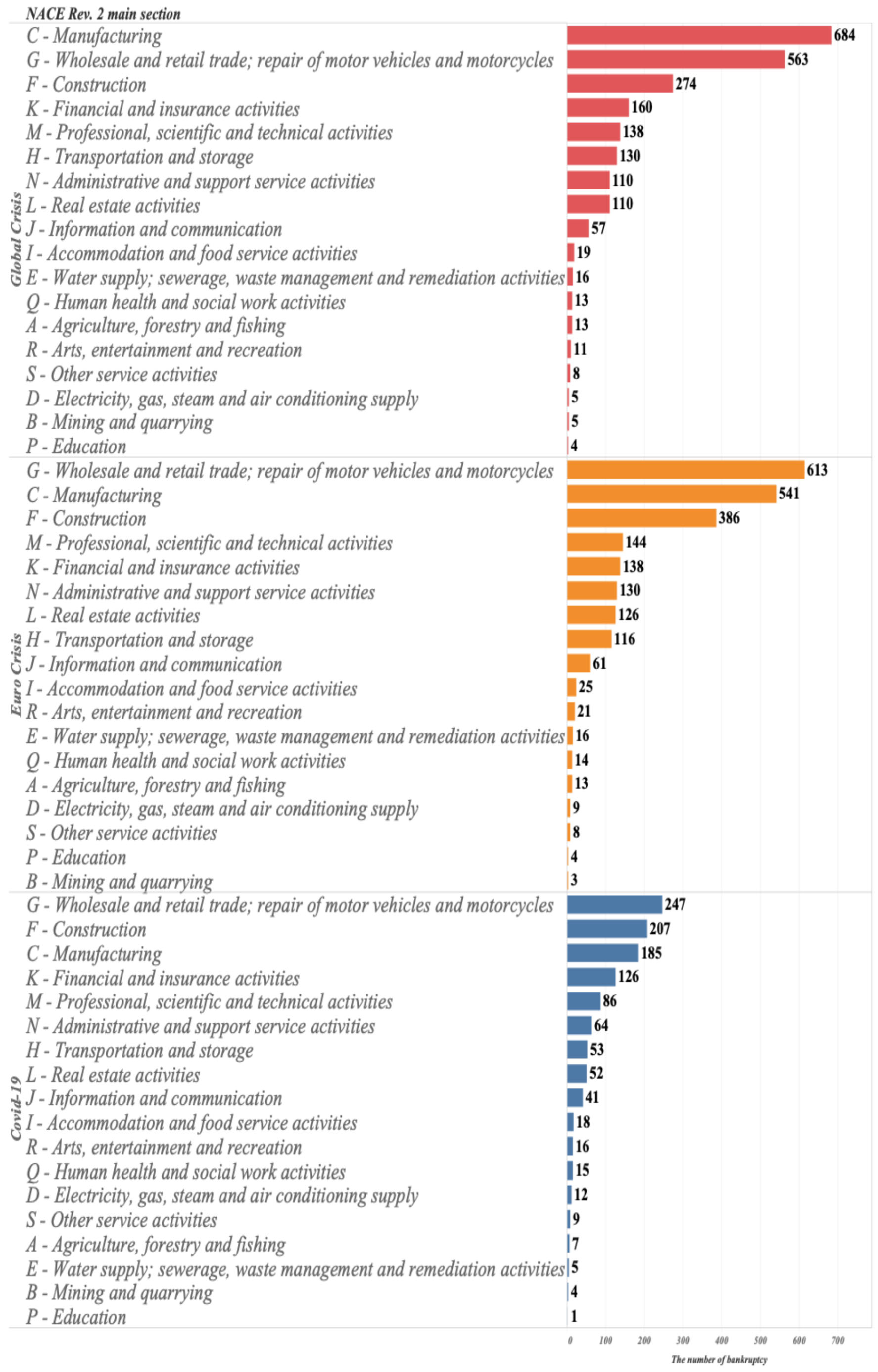
Figure A3 and Figure A4 in Appendix A illustrate the number of bankruptcy companies in each OECD country and industry. The country with the highest number of corporate bankruptcies during the Glob.C and EU.C is Italy, at 1057 and 1219, respectively. While not as severely affected as Italy, the Netherlands and France have been greatly impacted by the financial crisis compared to other countries during the two financial crises. The countries most affected by COVID are Italy and Sweden, as 279 bankruptcies are recorded in Orbis. As far as the Orbis record is concerned, Italy is the country most severely damaged by all economic crises.

We also define two tranquil events to compare how company bankruptcies during these crisis events differ from those during the tranquil period. To obtain more data, we set a longer timespan for the tranquil period, during which there were fewer bankrupt companies.

• Tranquil before Glob.C (preGlob.Trq), 2002–2006: The tranquil period prior to the Global Financial Crisis.
• Tranquil after EU.C (postEU.Trq), 2013–2018: The tranquil period after the European debt crisis.

3.2.2. Building Models

Following the same strategy as Tanaka et al. (2019), we built random forest models (Breiman 2001). Random forest is a nonlinear machine learning model and a variant of decision trees (Breiman et al. 1984), which is built by combining a large number of trees using random input selection instead of a single tree. We used random forest for the following reasons:

• It is simple but has strong predictive accuracy, has been well studied in the EWS literature, and reportedly outperforms conventional EWS approaches.
• The hyperparameter setting is extremely simple; it only requires a number of trees to construct the model, but it works with a large dataset as well as high-dimensional data efficiently and effectively.2
• It also has the convenience of dealing with multicollinearity, which causes interpretability problems owing to feature dependence in conventional methods such as logit, and tree models with univariate feature splits in general do not cause havoc, as each split is independent.
• Random forest also provides variable importance by measuring the relative contribution of variables to the prediction, which helps to identify and assess the criteria distinguishing different crises.

The algorithm of random forest is briefly explained as follows:

• Draw a subset of training data with random sampling by replacement (bootstrap).
• Train a decision tree using a subset of the training data. At each node of the tree, choose the best split of a variable from only the randomly selected m variables, rather than all variables.
• Repeat steps 1 and 2 to produce d decision trees.
• Make predictions for new data by voting for (or taking the average of) the most popular class from among all the outputs of d decision trees.

To obtain appropriate data to build our models, we clean the data by (1) removing indicators for which 70% of the values are missing and (2) removing companies for which more than 50% of financial statements are missing.

Table 1. The number of bankruptcy companies for each event.

Event	preGlob.Trq	Glob.C	EU.C	postEU.Trq	COV.C
Period	2002–2006	2007–2009	2010–2012	2013–2018	2019–2023
Data size	1694	2059	2202	2575	1021

shows the number of bankrupt companies collected for each event, and

Table 2. Global ratio indicators.

Type of Ratio	Ratios	1st Qu.	Median	Mean	3rd Qu.
Profitability	ROE using Profit (Loss) before tax	−11.33	2.03	−19.08	12.71
Ratios	ROCE using Profit (Loss) before tax	−10.47	2.28	−12.33	12.28
	ROA using Profit (Loss) before tax	−14.94	−1.89	−8.76	1.50
	ROE using Net income	−11.33	0.58	−27.41	6.34
	ROCE using Net income	−9.70	2.11	−15.38	9.75
	ROA using Net income	−14.30	−1.79	−9.40	0.72
	Profit margin	−9.93	−1.10	−7.53	0.91
	Gross margin	34.98	44.40	47.10	54.52
	EBITDA margin	−4.75	0.67	−1.90	3.65
	EBIT margin	−8.53	−0.28	−5.55	2.12
	Cash flow/Operating revenue	−5.57	0.05	−4.54	1.60
Operational	Net assets turnover	2.49	5.57	21.16	12.30
Ratios	Interest coverage	−5.15	−0.46	5.13	1.50
	Stock turnover	4.91	8.76	36.57	18.93
	Collection period days	24.00	59.00	90.71	113.00
	Credit period days	29.00	61.50	93.81	109.00
Structure	Current ratio	0.74	1.01	1.43	1.24
Ratios	Liquidity ratio	0.43	0.70	1.04	1.00
	Shareholders liquidity ratio	−0.02	0.47	7.92	1.94
	Solvency ratio (asset-based)	0.01	7.23	6.65	19.89
	Solvency ratio (liability-based)	8.22	13.14	17.52	19.09
	Gearing	95.53	134.58	185.82	181.84

lists the indicators and their statistics used to train our models.3 The data were randomly down-sampled to a smaller dataset for each model to balance the class distribution. The down-sampling approach may raise concerns about the loss of information; therefore, we decided to use only the original data for the comparison of models to avoid contaminating the dataset with noise caused by the oversampling approach. Nonetheless, the results using an oversampling approach are presented in Appendix B.

3.3. Evaluation

We evaluate and analyze the differences in bankruptcy among crises using model accuracy, variable importance, and partial dependency.

3.3.1. By Model Performance

We construct three binary models between two different events using random forest—Glob.C versus EU.C, Glob.C versus COV.C, and EU.C versus COV.C—and measure the accuracy of each model. Intuitively, if the mechanism of bankruptcy differs between the two crises, there should be different financial patterns in the data that can be detected by machine learning. The higher the accuracy of the model, the more distinguishable the data patterns between the two crises, implying the existence of different bankruptcy mechanisms between the two crises.

We also construct logistic regression models in the same setup to compare the performance of conventional methods and the random forest approach because random forest reportedly outperforms other methods in the EWS literature. The better random forest performance indicates a nonlinear relationship between the two crises.

If it is not possible to build accurate models using both random forest and logistic regression, there might be no distinct differences in bankruptcy mechanism, or more complex nonlinear modeling approaches are possibly required.

Furthermore, we evaluate the differences between tranquil periods by constructing six models: Glob.C, EU.C, and COV.C, versus preGlob.Trq and postEU.Trq.

For simplicity, we use the default number of trees in the H2O machine learning library. Model accuracy is reported as the average across 10-fold cross-validation. In 10-fold cross-validation, the dataset is randomly partitioned into 10 equal folds; in each iteration, a model is trained on 9 folds and evaluated on the held-out fold, yielding out-of-sample predictions for assessing generalization error.

3.3.2. By Variable Importance

Machine learning has great potential for building more accurate models, but is criticized for its lack of interpretability due to its black-box modeling nature. Accuracy is an incomplete description of tasks, especially for economic analysis, which mostly requires explanations as to why a certain decision is made regarding an event.

Random forest provides variable importance measurements (Breiman 2001), making its decision model construction process more interpretable. The important variables identified during the learning process of the random forest model indicate which variables have a greater influence on the prediction outcome. The importance of a variable is measured by comparing the original prediction error e_org with the prediction error e_perm after shuffling or permuting the values of the variable; hence, this method is also known as permutation variable importance. Intuitively, if the model’s prediction error, expressed as the quotient e_perm/e_org or difference e_perm − e_org, increases after shuffling, the feature is important because it indicates that the performance relies on the variable. However, if the two errors do not change significantly, the variable has little influence on the model performance; thus, it is unimportant.

Analyzing variable importance helps with understanding whether the models detect unique or common patterns or structures in the data. This provides confidence that the variables exert strong predictive signals. We analyzed the differences in criteria that distinguish crises based on variable importance.

3.3.3. By Partial Dependency

We further analyze the detailed relationship between the important variables found by each model and the prediction response based on one of the explainable artificial intelligence techniques called partial dependence plot (Friedman 2001).

The concept of partial dependency is to derive the behavior of the expected model prediction value as a function of the target explanatory variables by visualizing the average marginal effect of the target variables.4 The procedure for the partial dependence plot is as follows:

• Choose the target variable for which to create the partial dependence plot.
• Vary the value of the target variable while fixing the other values of the variables to create m datasets.
• Make a prediction output of each m dataset by model constructed.
• Plot the mean predicted value of each dataset of the target variable.

More formally, suppose we have a machine learning model $\widehat{f}\left(\mathbf{x}\right)$ trained on the dataset ${\left\{y_i,{\mathbf{x}}_i\right\}}_1^N$ of N instances, where y is a random response variable and x is a set of n random explanatory variables x = {$x_1,\dots ,x_n$}, the average partial dependency $\overline{f}\left(\mathit{x}\right)$ is defined as:

$$\overline{f}\left(x_s\right):=E_{{\mathbf{x}}_c}\left[\widehat{f}\left(x_s,{\mathit{x}}_C\right)\right]=\int \widehat{f}\left(x_s,{\mathit{x}}_C\right)p\left({\mathbf{x}}_C\right){d\mathbf{x}}_{\mathit{c}}$$

It provides a summary description of the dependence of $\widehat{f}\left(\mathit{x}\right)$ on the chosen subset of variables $x_s$ by plotting partial dependency, marginalizing over the complement subset ${\mathit{x}}_C$ ($x=x_s\cup x_c$, $x_s\cap x_c=\varnothing$). It is estimated from the training data as follows:

$$\overline{f}\left(x_s\right)={\displaystyle \frac{1}{N}}\sum _{i=1}^N\widehat{f}\left(x_s,x_{i,C}\right)$$

Partial dependency is obtained by averaging the marginal effects of the features and the response of all samples of the provided set.5

The partial dependence plot provides some insights into how a variable influences the predictions made by the model; the slope indicates the direction, whether it is a positive relationship, the strength of influence, and how steep it is. Another advantage of using a partial dependence plot with a machine learning-based model is that because it detects nonlinear relationships, it may be able to detect more complex relationships that are not detectable with simple models, such as linear regression models.

In this study, for simplicity, we use only the top three important variables identified by each model to conduct a partial dependency analysis.

4. Experimental Results

4.1. Analyzing Corporate Bankruptcy Differences Among Crises

This section examines whether the financial behavior associated with corporate bankruptcy differs across crises by assessing the performance of random forest and logistic regression models (hereafter referred to as RF and logit). We also analyze differences in financial indicators using variable importance measures and partial dependence plots.6 The two leftmost columns of

Table 3. Results of model accuracies.

		EU.C	COV.C	preGlob.Trq	postEU.Trq
rf	Glob.C	51.88%	68.47%	53.79%	60.60%
	EU.C		63.56%	57.62%	52.34%
	COV.C			74.15%	58.34%
glm	Glob.C	50.65%	56.79%	51.23%	51.42%
	EU.C		54.89%	52.03%	50.90%
	COV.C			56.46%	53.92%

report the RF and logit results for the three crises.

4.1.1. Glob.C Versus EU.C

Interestingly, the performance of both RF and logit (51.88% and 50.65%, respectively) is only about as good as random guessing. The results indicate that the financial behavior associated with corporate bankruptcy during the Glob.C and the EU.C does not differ in ways that can be captured by either linear or nonlinear models. This may be because the European debt crisis followed immediately after the global crisis, implying that the former was, in effect, a spillover from the latter.

The variable importance plot in Figure 1 shows that “Credit period days,” “Collection period days,” and “Gross margin” are the top three variables, yet none appear strong enough to distinguish the two crises. Most variables register relatively high importance, and the 13 variables collectively account for more than 0.7. These results suggest no substantial financial differences between firms that went bankrupt during the Glob.C and EU.C periods.

This can be seen more clearly in the partial dependence plots of the top three variables in Figure 2: their mean responses fluctuate only slightly, between about 0.46 and 0.50. Accordingly, changes in these values contribute little to predictive accuracy.

4.1.2. Glob.C Versus COV.C

In contrast to the Glob.C versus EU.C model, the RF model achieves high accuracy (68.47%). The results indicate that the financial behavior associated with corporate bankruptcy differs between the two events, implying different underlying drivers. The logit also performs above chance (56.79%), but its accuracy is roughly 12 percentage points lower than RF, suggesting that the differences are not well captured by linear models.

The variable importance plot in Figure 3 shows that “Collection period days” and “Credit period days” are the two most important variables for distinguishing the Glob.C from the COV.C. These are the same variables highlighted in the Glob.C versus EU.C case; however, unlike that comparison—which lacked dominant variables—here they emerge as clearly more influential. Furthermore, “Cash flow/Operating revenue” and “Liquidity ratio” rank 3rd and 4th, whereas they ranked 13th and 14th, respectively, in the Glob.C versus EU.C model. Despite the prominence of the top two variables, “Cash flow/Operating revenue,” “Liquidity ratio,” and “Solvency ratio (asset-based)” also show relatively high contributions (≈0.7), and the next three variables are around 0.6. These mixed contributions underscore the complexity of the bankruptcy mechanisms distinguishing the Glob.C from the COV.C. By comparison, in the Glob.C versus EU.C model, many variables exhibited similarly high contributions, implying that no single variable distinctly characterizes the difference between those events.

The partial dependence plots in Figure 4 show that as “Collection period days” and “Credit period days” increase, the probability of the Glob.C rises and then stabilizes after approximately 207 and 155 days, respectively. By contrast, “Cash flow/Operating revenue” behaves differently: the probability of the Glob.C drops sharply when this ratio falls to around −24%. Thus, the lengths of “Collection period days” and “Credit period days,” as well as the sign and magnitude of “Cash flow/Operating revenue,” characterize the differences between the two crises: longer collection and credit periods have a greater impact on the Glob.C, and the Glob.C is more sensitive to negative “Cash flow/Operating revenue” than the COV.C.

4.1.3. EU.C Versus COV.C

Similar to the Glob.C versus COV.C case, model accuracy exceeds random guessing—63.56% for the RF model and 54.89% for the logit model. Although RF accuracy is not as high as in the Glob.C–COV.C comparison, there are still distinguishable differences in the financial mechanisms of corporate bankruptcy between EU.C and COV.C. The difference between RF and logit further suggests that nonlinear relationships explain these events more effectively than linear ones.

The top three variables in Figure 5—“Credit period days,” “Collection period days,” and “Cash flow/Operating revenue”—are the same as in the Glob.C–COV.C case, although ranked slightly differently. The most important and dominant variable in the EU.C–COV.C comparison is “Credit period days,” whereas in the Glob.C–COV.C case, “Credit period days” and “Collection period days” contributed almost equally. The top five variables also remain the same, except that the fourth position switches between “ROA (using net income)” and “Liquidity ratio.” However, their contributions to distinguishing the EU.C and Glob.C from the COV.C differ markedly: while the Glob.C–COV.C model has nine variables with importance above 0.6 (five above 0.7), the EU.C–COV.C model has only three above 0.6, and most variables do not materially affect the distinction in financial behavior between the EU.C and COV.C.

These results indicate that “Credit period days” and “Collection period days” effectively explain differences in bankruptcy mechanisms between the Glob.C/EU.C and the COV.C. In particular, these variables strongly drive the distinguishability of the EU.C versus the COV.C, whereas additional factors in the Glob.C–COV.C model improve accuracy and suggest a slightly more complex mechanism. This may reflect the timespan: the EU.C is closer in time to the COV.C than the Glob.C, and may have unfolded under different economic conditions.

The partial dependence plots in Figure 6 mirror those in the Glob.C–COV.C model. The probability of the EU.C increases as “Credit period days” and “Collection period days” lengthen, peaking at around 210 and 204 days, respectively. By contrast, a decline in “Cash flow/Operating revenue”—although not as sharp as in the Glob.C–COV.C case—reduces the probability of the EU.C. Again, the lengths of “Collection period days” and “Credit period days,” together with the sign of “Cash flow/Operating revenue,” characterize the differences between the two crises.

4.2. Analyzing Corporate Bankruptcy Differences Among Crises and Tranquil Periods in Chronological Order

Variations in key financial indicators across crises may reflect differences in the nature of each shock. For instance, during COVID-19, firms may have faced sudden revenue halts due to lockdowns, making liquidity ratios more critical. By contrast, during the Global Financial Crisis, credit availability and receivables collection likely played a more dominant role, highlighting the relevance of “Credit period days” and “Collection period days” in explaining bankruptcy risk.

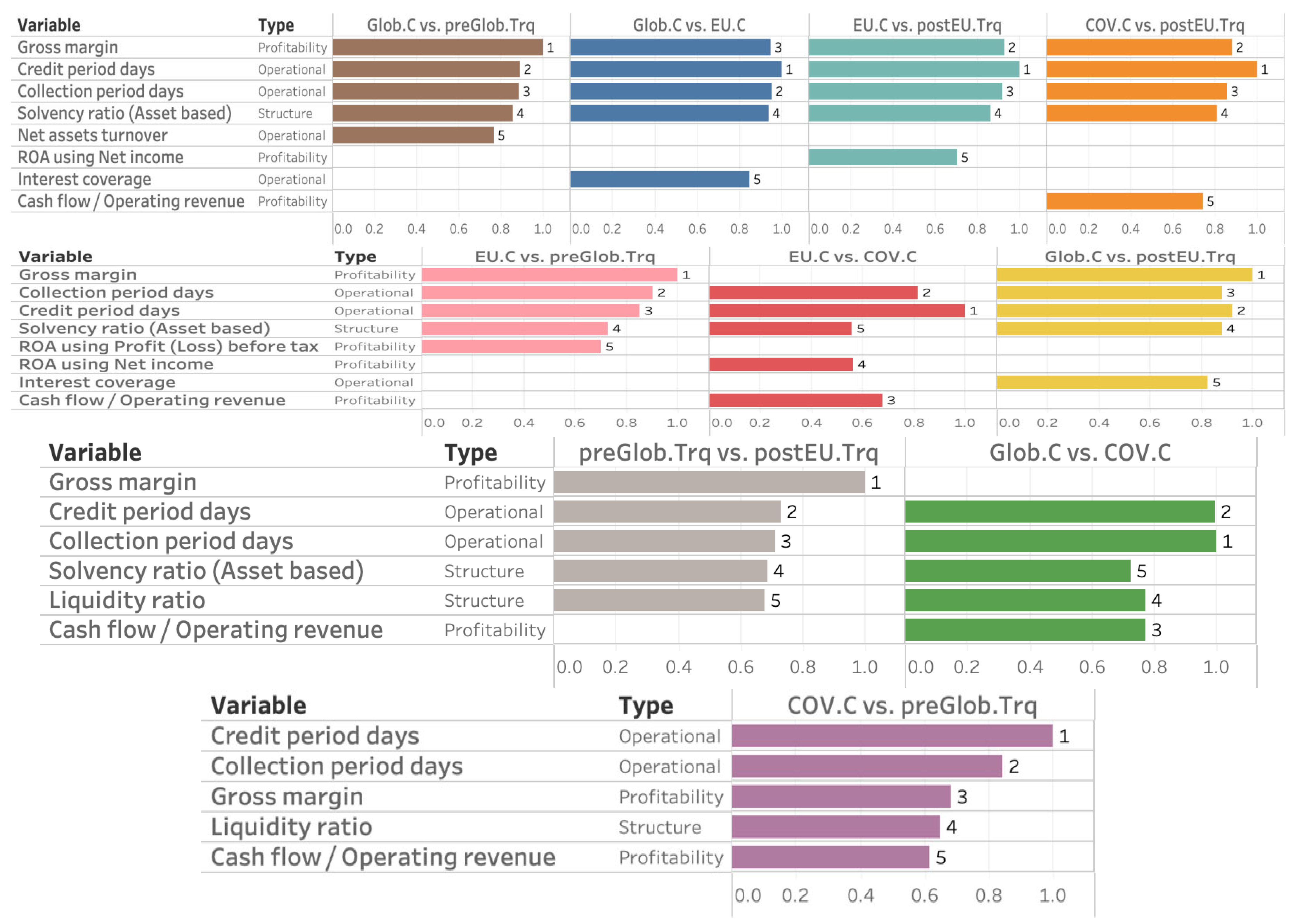
Our experimental results have important implications for the financial behavior of corporate bankruptcy in both crisis and tranquil periods. Figure 7 presents the RF model results in chronological order. Figure 8 shows the important variables identified between pairs of events based on chronological distance, with each row corresponding to the third, second, fourth, and fifth arches from the top in Figure 7. The first row describes adjacent events: Glob.C versus preGlob.Trq, Glob.C versus EU.C, EU.C versus postEU.Trq, and COV.C versus postEU.Trq. The second row describes every other event: EU.C versus preGlob.Trq, EU.C versus COV.C, and Glob.C versus postEU.Trq. The third and fourth rows describe more distant events: preGlob.Trq versus postEU.Trq, Glob.C versus COV.C, and COV.C versus preGlob.Trq. The experimental findings are summarized as follows:

• Model accuracies for adjacent events are only slightly above 50%—marginally better than random guessing—except for the postEU.Trq versus COV.C model, which is nearly 60%. This suggests that the financial behavior associated with bankruptcy in adjacent events does not vary markedly from the preGlob.Trq to postEU.Trq models, whereas the COV.C bankruptcy mechanism exhibits more distinguishable characteristics than in previous events.
• In contrast, model accuracy for the every-other-event comparisons was consistently around 60%. These results imply that bankruptcy-related financial behavior changes after certain events and becomes more pronounced between more distant events. Because corporate activity is closely related to overall economic activity, our results may reflect structural changes in the economy over 2002–2023. It is not certain whether each event changes bankruptcy-related financial behavior, economic conditions, and/or firms’ financial management policies; further investigation is required and left for future research.
• The results indicate that COV.C has a distinct bankruptcy mechanism compared with previous events, as evidenced by the ability to construct a high-accuracy model. “Cash flow/Operating revenue” is a key distinguishing factor between COV.C and the other events—namely, the Glob.C, EU.C, preGlob.Trq, and postEU.Trq. Further investigation is required to determine whether this variable is also a key factor in other crises.
• Because linear models cannot adequately distinguish such disparities in financial mechanisms—the logit approach, in particular, yields low-accuracy models—it is crucial to consider nonlinear methods, such as our random forest framework, when analyzing distinctions across crises.
• Irrespective of chronological distance, the four most important variables distinguishing crisis from tranquil periods are extremely similar: “Credit period days,” “Gross margin,” “Collection period days,” and “Solvency ratio (asset-based).” In particular, “Gross margin” may be a key indicator for monitoring transitions between tranquil and crisis periods, as it does not appear among the top variables in the EU.C–COV.C and Glob.C–COV.C models. Notwithstanding the overall accuracy figures, some models perform only about as well as random guessing. Although these factors can detect crisis versus tranquil periods, predictive accuracy varies with their relative contributions; hence, their contribution is the key driver of accuracy.7
• Hence, even when adjacent events show little difference over a given period, it remains important to monitor preceding events because the bankruptcy mechanism can change abruptly, as in the COV.C. More importantly, our results demonstrate the value of monitoring the bankruptcy behavior of the event immediately preceding the latest event.
• Furthermore, Credit period day, Collection period day, and Cashflow/Operating revenue are repeatedly identified as important indicators.8 These factors represent the liquidity at hand and a liquidity condition not reflected in the Profit and Loss statement or Balance Sheet. For instance, phenomena such as surplus bankruptcy are suggested by three indicators. This study found that the differences in liquidity depletion within a company may indicate the difference. Specifically, this study suggests that the bankruptcy mechanisms of the global and European financial crises, as well as the economic crisis caused by the COVID pandemic, are not due to insolvency but rather to factors related to liquidity. The depletion of liquidity within a company can indicate the severity of a crisis.
• Our models are built on a crisis-focused dataset and are therefore influenced by the Global Financial Crisis (Glob.C), the European debt crisis (EU.C), and the COVID-19 crisis (COV.C). They are also affected by the distribution of bankruptcies across countries and industries in the dataset; for example, countries such as Italy, France, and the Netherlands, and industries such as C—Manufacturing and G—Wholesale and Retail Trade; Repair of Motor Vehicles and Motorcycles, show relatively high numbers of bankruptcies. Despite these context-specific factors, our analytical framework enables us to identify differences in bankruptcy mechanisms across crises—something that simple bankrupt versus nonbankrupt analyses cannot achieve. Accordingly, it may serve as an alternative early warning system.

5. Conclusions

This study investigated how bankruptcy mechanisms differ across major crises—the Global Financial Crisis, the European debt crisis, and the COVID-19 crisis—by leveraging firm-level financial data and machine learning techniques. It contributes to the literature on economic crisis analysis by examining the financial behavior of corporate bankruptcy during crisis periods. Unlike conventional early warning systems (EWS) frameworks (Jayasekera 2018; Tanaka et al. 2019; Stewart et al. 2017; Barboza et al. 2017; Holopainen and Sarlin 2017), which analyze differences between nonbankrupt and bankrupt companies, this study focuses exclusively on bankrupt companies. We introduce a framework based on a random forest model, exploiting a corporate bankruptcy dataset from 2002 to 2023 that spans three crises and two tranquil periods, and investigate (1) whether the financial mechanisms of corporate bankruptcy differ among the Global Financial Crisis, the European debt crisis, and the COVID-19 crisis; (2) whether these crises differ from tranquil periods—specifically the pre-Global Financial Crisis and post-European debt crisis periods; and (3) how they differ.

The findings indicate that the mechanisms underpinning bankruptcy in the Global Financial Crisis and the European debt crisis are similar, whereas those in the COVID-19 crisis differ markedly. Our results further suggest abrupt, nonlinear shifts in financial behavior. Accordingly, a nonlinear modeling framework is essential for detecting such changes. We also find that “Credit period days,” “Collection period days,” “Gross margin,” and “Solvency ratio (asset-based)” are key factors distinguishing these events. In particular, the COVID-19 crisis displays a distinct bankruptcy mechanism, as reflected in the high predictive accuracy achievable during that period.

Our framework is flexible and can be adapted to other financial datasets and machine learning methods, such as gradient boosting (Friedman 2001) and XGBoost (Chen and Guestrin 2016). It also allows relatively straightforward hyperparameter tuning and facilitates model interpretation (e.g., variable importance and partial dependence plots).

This study has several limitations. First, our analysis focuses on larger firms in the OECD. Analyzing small- and medium-sized enterprises is also important, given their prevalence and the cumulative macroeconomic effects of their failures. Second, we do not incorporate country-specific macroeconomic conditions; a more comprehensive analysis would include factors such as policy rates, credit spreads, and policy responses. Third, the number of bankrupt firms is not sufficiently large to fully uncover crisis-specific mechanisms. While data augmentation using advanced methods (e.g., generative deep learning) could be considered, it warrants caution due to potential distributional distortion and leakage risks; extending the sample period and integrating additional data sources are preferable first steps.

Corporate activity plays a crucial role in maintaining economic stability. In practice, decision-makers often need to make forward-looking judgments to anticipate economic trends, for which analyzing cross-crisis differences in bankruptcy mechanisms can be useful. Earlier crises not covered here (e.g., Japan’s asset-price bubble and the dot-com bubble), as well as recent geopolitical risks and extreme weather, have had material adverse effects on the global economy. Extending the analysis to these episodes remains an avenue for future research.

Our findings provide actionable guidance for enhancing early warning systems (EWS) and credit-risk frameworks by incorporating crisis-specific financial indicators—particularly “Credit/Collection period days,” “Gross margin,” and “Solvency ratio (asset-based)”—into monitoring dashboards to improve early alerts and supervisory triage. To support deployment at scale, future research should validate transferability across countries and industries and assess robustness under varying macroeconomic conditions and firm sizes.

References

1. Acharya, Viral V., Lasse H. Pedersen, Thomas Philippon, and Matthew Richardson. 2017. Measuring Systemic Risk. The Review of Financial Studies 30: 2–47. [Google Scholar] [CrossRef]
2. Alpaydin, Ethem. 2014. Introduction to Machine Learning. Cambridge, MA: The MIT Press. [Google Scholar]
3. Altman, Edward I. 1968. Financial Ratios, Discriminant Analysis and the Prediction of Corporate Bankruptcy. The Journal of Finance 23: 589–609. [Google Scholar] [CrossRef]
4. Altman, Edward I. 1984. The Success of Business Failure Prediction Models: An International Survey. Journal of Banking & Finance 8: 171–98. [Google Scholar]
5. Altman, Edward I. 1993. Corporate Financial Distress and Bankruptcy: A Complete Guide to Predicting and Avoiding Distress and Profiting from Bankruptcy, Wiley Finance ed. New York: Wiley, vol. 18.3. [Google Scholar]
6. Altman, Edward I., Giancarlo Marco, and Franco Varetto. 1994. Corporate Distress Diagnosis: Comparisons Using Linear Discriminant Analysis and Neural Networks (the Italian Experience). Journal of Banking & Finance 18: 505–29. [Google Scholar] [CrossRef]
7. Altman, Edward I., Małgorzata Iwanicz-Drozdowska, Erkki K. Laitinen, and Arto Suvas. 2017. Financial Distress Prediction in an International Context: A Review and Empirical Analysis of Altman’s z-Score Model. Journal of International Financial Management & Accounting 28: 131–71. [Google Scholar]
8. Barboza, Flavio, Herbert Kimura, and Edward Altman. 2017. Machine Learning Models and Bankruptcy Prediction. Expert Systems with Applications 83: 405–17. [Google Scholar] [CrossRef]
9. Beaver, William H. 1966. Financial Ratios as Predictors of Failure. Journal of Accounting Research 4: 71–11. [Google Scholar] [CrossRef]
10. Berger, Allen N., and Christa H. S. Bouwman. 2013. How Does Capital Affect Bank Performance During Financial Crises? Journal of Financial Economics 109: 146–76. [Google Scholar] [CrossRef]
11. Beutel, Johannes, Sophia List, and Gregor von Schweinitz. 2019. Does Machine Learning Help Us Predict Banking Crises? Journal of Financial Stability 45: 100693. [Google Scholar] [CrossRef]
12. Bitetto, Alessandro, Paola Cerchiello, and Charilaos Mertzanis. 2023. Measuring Financial Soundness Around the World: A Machine Learning Approach. International Review of Financial Analysis 85: 102451. [Google Scholar] [CrossRef]
13. Breiman, Leo. 2001. Random Forests. Machine Learning 45: 5–32. [Google Scholar] [CrossRef]
14. Breiman, Leo, Jerome Friedman, Charles J. Stone, and Richard A. Olshen. 1984. Classification and Regression Trees. In Monterey: Wadsworth. London: Chapman & Hall. [Google Scholar]
15. Brédart, Xavier. 2014. Bankruptcy Prediction Model: The Case of the United States. International Journal of Economics and Finance 6: 1–7. [Google Scholar] [CrossRef]
16. Brownlees, Christian, and Robert F. Engle. 2016. SRISK: A Conditional Capital Shortfall Measure of Systemic Risk. The Review of Financial Studies 30: 48–79. [Google Scholar] [CrossRef]
17. Bussiere, Matthieu, and Marcel Fratzscher. 2006. Towards a New Early Warning System of Financial Crises. Journal of International Money and Finance 25: 953–73. [Google Scholar] [CrossRef]
18. Campbell, John Y., Jens Hilscher, and Jan Szilagyi. 2008. In Search of Distress Risk. The Journal of Finance 63: 2899–939. [Google Scholar] [CrossRef]
19. Chakraborty, Sumit, and Sushil K. Sharma. 2007. Prediction of Corporate Financial Health by Artificial Neural Network. International Journal of Electronic Finance 1: 442–59. [Google Scholar] [CrossRef]
20. Chava, Sudheer, and Robert A. Jarrow. 2004. Bankruptcy Prediction with Industry Effects. Review of Finance 8: 537–69. [Google Scholar] [CrossRef]
21. Chawla, Nitesh V., Kevin W. Bowyer, Lawrence O. Hall, and W. Philip Kegelmeyer. 2002. SMOTE: Synthetic Minority Over-sampling Technique. Journal of Artificial Intelligence Research 16: 321–57. [Google Scholar] [CrossRef]
22. Chen, Tianqi, and Carlos Guestrin. 2016. XGBoost: A Scalable Tree Boosting System. Paper presented at KDD ’16: 22nd ACM SIGKDD International Conference on Knowledge Discovery and Data Mining, San Francisco, CA, USA, August 13–17; New York: Association for Computing Machinery, pp. 785–94. [Google Scholar]
23. Claessens, Stijn, and Neeltje van Horen. 2015. The Impact of the Global Financial Crisis on Banking Globalization. DNB Working Papers 459. Amsterdam: Netherlands Central Bank, Research Department. [Google Scholar]
24. Cleary, Sean, and Greg Hebb. 2016. An Efficient and Functional Model for Predicting Bank Distress: In and Out of Sample Evidence. Journal of Banking & Finance 64: 101–11. [Google Scholar] [CrossRef]
25. Climent, Francisco, Alexandre Momparler, and Pedro Carmona. 2019. Anticipating Bank Distress in the Eurozone: An Extreme Gradient Boosting Approach. Journal of Business Research 101: 885–96. [Google Scholar] [CrossRef]
26. Demirguc-Kunt, Asli, Enrica Detragiache, and Ouarda Merrouche. 2013. Bank Capital: Lessons from the Financial Crisis. Journal of Money Credit and Banking 45: 1147–64. [Google Scholar] [CrossRef]
27. Drehmann, Mathias, and Mikael Juselius. 2014. Evaluating Early Warning Indicators of Banking Crises: Satisfying Policy Requirements. International Journal of Forecasting 30: 759–80. [Google Scholar] [CrossRef]
28. Drehmann, Mathias, and Nikola Tarashev. 2013. Measuring the Systemic Importance of Interconnected Banks. Journal of Financial Intermediation 22: 586–607. [Google Scholar] [CrossRef]
29. Einav, Liran, and Jonathan Levin. 2014. The Data Revolution and Economic Analysis. Innovation Policy and the Economy 14: 1–24. [Google Scholar] [CrossRef]
30. Frankel, Jeffrey A., and Andrew K. Rose. 1996. Currency crashes in emerging markets: An empirical treatment. Journal of International Economics 41: 351–66. [Google Scholar] [CrossRef]
31. Frankel, Jeffrey A., and George Saravelos. 2010. Are Leading Indicators of Financial Crises Useful for Assessing Country Vulnerability? Evidence from the 2008 Global Crisis. Working Paper 16047. Working Paper Series; Cambridge, MA: National Bureau of Economic Research. [Google Scholar]
32. Frankel, Jeffrey A., and Shang-Jin Wei. 2004. Managing Macroeconomic Crises. Working Paper 10907. Working Paper Series; Cambridge, MA: National Bureau of Economic Research. [Google Scholar]
33. Frankel, Jeffrey, and George Saravelos. 2012. Can Leading Indicators Assess Country Vulnerability? Evidence from the 2008–09 Global Financial Crisis. Journal of International Economics 87: 216–31. [Google Scholar] [CrossRef]
34. Friedman, Jerome H. 2001. Greedy Function Approximation: A Gradient Boosting Machine. Annals of Statistics 29: 1189–23. [Google Scholar] [CrossRef]
35. Geron, Aurelien. 2022. Hands-On Machine Learning with Scikit-Learn, Keras, and TensorFlow: Concepts, Tools, and Techniques to Build Intelligent Systems, 3rd ed. Sebastopol: O’Reilly Media, Inc. [Google Scholar]
36. Ghosh, Swart R., and Atish R. Ghosh. 2002. Structural Vulnerabilities and Currency Crises. IMF Working Papers 02/9. Washington, DC: International Monetary Fund. [Google Scholar]
37. Hillegeist, Stephen A., Elizabeth K. Keating, Donald P. Cram, and Kyle G. Lundstedt. 2004. Assessing the Probability of Bankruptcy. Review of Accounting Studies 9: 5–34. [Google Scholar] [CrossRef]
38. Holopainen, Markus, and Peter Sarlin. 2017. Toward Robust Early-Warning Models: A Horse Race, Ensembles and Model Uncertainty. Quantitative Finance 17: 1933–63. [Google Scholar] [CrossRef]
39. Jayasekera, Ranadeva. 2018. Prediction of Company Failure: Past, Present and Promising Directions for the Future. International Review of Financial Analysis 55: 196–208. [Google Scholar] [CrossRef]
40. Joy, Mark, Marek Rusnák, Kateřina Šmídková, and Bořek Vašíček. 2017. Banking and Currency Crises: Differential Diagnostics for Developed Countries. International Journal of Finance & Economics 22: 44–67. [Google Scholar]
41. Kim, Choong Nyoung, Kyung Hoon Yang, and Jaekyung Kim. 2008. Human Decision-Making Behavior and Modeling Effects. Decision Support Systems 45: 517–27. [Google Scholar] [CrossRef]
42. Kristóf, Tamás, and Miklós Virág. 2022. EU-27 Bank Failure Prediction with C5.0 Decision Trees and Deep Learning Neural Networks. Research in International Business and Finance 61: 101644. [Google Scholar] [CrossRef]
43. Lennox, Clive. 1999. Identifying Failing Companies: A Re-Evaluation of the Logit, Probit and DA Approaches. Journal of Economics and Business 51: 347–64. [Google Scholar] [CrossRef]
44. Liu, Jiaming, Chengzhang Li, Peng Ouyang, Jiajia Liu, and Chong Wu. 2023. Interpreting the Prediction Results of the Tree-Based Gradient Boosting Models for Financial Distress Prediction with an Explainable Machine Learning Approach. Journal of Forecasting 42: 1112–37. [Google Scholar] [CrossRef]
45. Martin, Daniel. 1977. Early Warning of Bank Failure: A Logit Regression Approach. Journal of Banking & Finance 1: 249–76. [Google Scholar]
46. Messier, William F., and James V. Hansen. 1988. Inducing Rules for Expert System Development: An Example Using Default and Bankruptcy Data. Management Science 34: 1403–15. [Google Scholar] [CrossRef]
47. Oet, Mikhail V., Timothy Bianco, Dieter Gramlich, and Stephen J. Ong. 2013. SAFE: An Early Warning System for Systemic Banking Risk. Journal of Banking & Finance 37: 4510–13. [Google Scholar] [CrossRef]
48. Ohlson, James A. 1980. Financial Ratios and the Probabilistic Prediction of Bankruptcy. Journal of Accounting Research 18: 109. [Google Scholar] [CrossRef]
49. Rose, Andrew K., and Mark M. Spiegel. 2011. Cross-country causes and consequences of the crisis: An update. European Economic Review 55: 309–24. [Google Scholar] [CrossRef]
50. Shirata, Cindy. 2003. Predictors of Bankruptcy After Bubble Economy in Japan: What Can You Learn from Japan Case? Paper presented at 15th Asian-Pacific Conference on International Accounting Issues, Bangkok, Thailand, November 24. [Google Scholar]
51. Shumway, Tyler. 2001. Forecasting Bankruptcy More Accurately: A Simple Hazard Model. The Journal of Business 74: 101–24. [Google Scholar] [CrossRef]
52. Silva, Walmir, Herbert Kimura, and Vinicius Amorim Sobreiro. 2017. An Analysis of the Literature on Systemic Financial Risk: A Survey. Journal of Financial Stability 28: 91–114. [Google Scholar] [CrossRef]
53. Stewart, Jones, Johnstone David, and Wilson Roy. 2017. Predicting Corporate Bankruptcy: An Evaluation of Alternative Statistical Frameworks. Journal of Business Finance & Accounting 44: 3–34. [Google Scholar]
54. Tanaka, Katsuyuki, Takuji Kinkyo, and Shigeyuki Hamori. 2016. Random Forests-Based Early Warning System for Bank Failures. Economics Letters 148: 118–21. [Google Scholar] [CrossRef]
55. Tanaka, Katsuyuki, Takuji Kinkyo, and Shigeyuki Hamori. 2018. Financial Hazard Map: Financial Vulnerability Predicted by a Random Forests Classification Model. Sustainability 10: 1530. [Google Scholar] [CrossRef]
56. Tanaka, Katsuyuki, Takuo Higashide, Takuji Kinkyo, and Shigeyuki Hamori. 2019. Analyzing Industry-Level Vulnerability by Predicting Financial Bankruptcy. Economic Inquiry 57: 2017–34. [Google Scholar] [CrossRef]
57. Tian, Shaonan, and Yan Yu. 2017. Financial Ratios and Bankruptcy Predictions: An International Evidence. International Review of Economics & Finance 51: 510–26. [Google Scholar] [CrossRef]
58. Tola, Albi, and Sebastien Waelti. 2018. Financial Crises, Output Losses, and the Role of Structural Reforms. Economic Inquiry 56: 761–98. [Google Scholar] [CrossRef]
59. Varian, Hal R. 2014. Big Data: New Tricks for Econometrics. Journal of Economic Perspectives 28: 3–28. [Google Scholar] [CrossRef]
60. Vazquez, Francisco, and Pablo Federico. 2015. Bank Funding Structures and Risk: Evidence from the Global Financial Crisis. Journal of Banking & Finance 61: 1–14. [Google Scholar] [CrossRef]
61. Ward, Felix. 2017. Spotting the Danger Zone: Forecasting Financial Crises with Classification Tree Ensembles and Many Predictors. Journal of Applied Econometrics 32: 359–78. [Google Scholar] [CrossRef]
Figure 1. Variable importance in the Glob.C versus EU.C model.
Risks 13 00158 g001
Figure 2. Partial dependence plot of the top three important variables in the Glob.C versus EU.C model. Mean response represents the probability of being Glob.C.
Risks 13 00158 g002
Figure 3. Variable importance in the Glob.C versus COV.C model.
Risks 13 00158 g003
Figure 4. Partial dependence plot of the top three important variables in the Glob.C versus COV.C model. Mean response represents the probability of being a Glob.C.
Risks 13 00158 g004
Figure 5. Variable importance in the EU.C versus COV.C model.
Risks 13 00158 g005
Figure 6. Partial dependence plot of the top three important variables in the EU.C versus COV.C model. Mean response represents the probability of being a COV.C.
Risks 13 00158 g006
Figure 7. Bankruptcy model accuracies in chronological order.
Risks 13 00158 g007
Figure 8. Summary of the top five important variables for each model.
Risks 13 00158 g008