Abstract
This study investigates whether green assets can serve as safe havens for dirty assets in the context of carbon and energy futures markets. Using daily data from April 2021 to June 2025, the analysis focuses on four key instruments: carbon emissions futures and crude oil futures, EUA futures, and natural gas futures. The study applies two main approaches—a conditional value-at-risk (CVaR)-based relative risk ratio (RRR) analysis and dynamic conditional correlation (DCC-GARCH) modeling—to assess tail risk mitigation and time-varying correlations. The results show that while green assets do not consistently act as safe havens during extreme market downturns, they can reduce the portfolio tail risk beyond certain allocation thresholds. Natural gas futures demonstrate significant volatility but offer diversification benefits when their portfolio weight exceeds 40%. EUA futures, although highly correlated with carbon emissions futures, show limited safe haven behavior. The findings challenge the assumption that green assets inherently provide downside protection and highlight the importance of strategic allocation. This research contributes to the literature by extending safe haven theory to environmental futures and offering empirical insights into the risk dynamics between green and dirty assets.
1. Introduction
Crude oil is a critical input for modern economies, shaping production costs, trade balances, and national energy security. It is a vital input for economic development, and its pricing plays a central role in global financial stability. Given its strategic importance, fluctuations in international spot prices have posed significant economic hazards for both governments and markets. In response to these risks, futures markets were established to enhance price discovery, manage volatility, and provide greater transparency. A major institutional development in this regard was the launch of crude oil futures contracts by the New York Mercantile Exchange (NYMEX) in 1983 and the London Intercontinental Exchange in 1988 (Tian and Lai 2019). Notably, the NYMEX contract, introduced in March 1983 (Gülen 1998), specified physical delivery at Cushing, Oklahoma, and became benchmarked primarily against West Texas Intermediate (WTI), which has since evolved into a global reference price for crude oil. Today, most crude oil is traded through futures markets, where derivatives often have a greater influence on price discovery than physical transactions. Since oil is priced in U.S. dollars, fluctuations in exchange rates—especially dollar depreciation—can significantly affect oil prices. These dynamics highlight the interconnected nature of energy and currency markets and the strategic importance of futures trading in managing volatility and economic risk (Sun et al. 2022).
Natural gas, like crude oil, plays a vital role in the global energy system due to its cleaner combustion and lower greenhouse gas emissions. Its growing use across residential, industrial, and power sectors, along with its rising share in global energy demand, underscores its strategic importance alongside oil in both national energy policies and international markets. According to the International Energy Agency, natural gas consumption grew by 4.6% in 2018, accounting for nearly half of the global increase in energy demand, and projections show current levels increasing by 2040, with natural gas continuing to outperform coal and oil (IEA 2019). These trends highlight why natural gas and crude oil remain central to discussions on energy security, economic development, and environmental transition. With the rise of financial globalization, understanding how returns and volatility are transmitted across capital markets has become increasingly important. Fluctuations in natural gas, crude oil, and electricity indices have to be investigated to unveil the risk and value of investment portfolios (Zhang et al. 2020).
However, the widespread use of crude oil has also contributed significantly to global CO2 emissions and environmental degradation, prompting growing concern among policy-makers. In response, international agreements such as the Paris Agreement have emerged, aiming to curb greenhouse gas emissions and accelerate the transition to cleaner energy sources. The Kyoto Protocol required industrialized countries to reduce greenhouse gas emissions by about 5% below 1990 levels during 2008–2012. To support this goal, it introduced three international cooperation mechanisms, including carbon trading (Wei and Lin 2016). One key tool was the Emission Trading Scheme (ETS), targeting energy-intensive sectors and households. Within this system, polluting industries received tradable carbon emission rights known as European Union Allowances (EUAs), allowing them to emit a set amount of CO2 annually. The carbon market responds to overall energy market developments; as a result, it could serve as a hedge or a safe haven tool against U.S. climate policy uncertainty (CPU). A weak (strong) hedge occurs when an asset is uncorrelated (positively correlated) with U.S. climate policy uncertainty, and a weak (strong) safe haven exists when an asset is uncorrelated (positively correlated) with U.S. CPU during periods of market stress (Hoque and Batabyal 2022). Furthermore, Shaton et al. (2020) finds that clean energy stocks significantly offset the downside risks associated with dirty energy stocks, and this protective effect persists even during times of market movements. Natural gas is often introduced as a transitional energy source in climate policy discussions. One of its main advantages is its potential to reduce greenhouse gas (GHG) emissions, as burning an equivalent energy unit of natural gas emits roughly half the CO2 compared to coal or oil (Shaton et al. 2020). Although it still represents a continued reliance on fossil fuels, natural gas is expected to contribute to emission reductions over the coming decades (Pacala and Socolow 2004; Howarth et al. 2011). In light of these considerations, this study focuses on carbon emissions futures, crude oil WTI futures, European Union Allowance (EUA) futures, and natural gas futures, as they represent key instruments for examining safe haven theory between dirty and green assets in the context of carbon and energy futures markets.
This study is guided by the following research question: Can green energy futures serve as safe havens for dirty energy futures under extreme market conditions? To address this, we test two hypotheses:
H1.
Green assets act as safe havens during extreme downturns.
H2.
Green assets reduce portfolio tail risk when allocated above certain thresholds.
This study treats carbon emissions futures as a dirty asset indicator and EUA futures as a green asset. While carbon emissions futures primarily reflect the financialization of pollution without enforcing actual reductions, EUA futures are embedded in the EU’s binding cap-and-trade system, designed to drive emissions down. Accordingly, these variables are considered within the analytical framework to reflect opposing signals: one aligned with speculative pollution trading, the other with regulatory decarbonization efforts. Additionally, crude oil futures are considered a dirty asset indicator, while natural gas futures are treated as a green asset. Crude oil futures are linked to high carbon intensity and are widely associated with substantial CO2 emissions, reflecting continued dependence on carbon-intensive energy sources. In contrast, natural gas futures are viewed as relatively cleaner due to their lower carbon output per energy unit, positioning them as part of the transition toward less polluting energy alternatives.
The data set spans from 1 April 2021 to 25 June 2025 and includes assets from both European and U.S. markets. Specifically, EUA futures and carbon credits represent the European segment, while clean energy ETFs and natural gas futures are sourced from U.S. exchanges. This cross-regional selection enables a broader assessment of green asset dynamics across major energy and carbon markets.
These assets are widely utilized as investment instruments in financial markets, offering exposure to the energy and environmental sectors. However, due to their sensitivity to geopolitical events, regulatory changes, and macroeconomic dynamics, they are often subject to considerable price volatility. In response to such fluctuations, investors may seek safe haven assets to protect their portfolios during periods of heightened uncertainty. In this context, some market participants might perceive one of the four futures contracts examined in this study as a potential safe haven relative to another. To test the safe haven properties, we followed the methodological steps employed by Kuang (2021). In that study, Kuang investigated the safe haven relationship between clean and dirty cryptocurrencies by applying a model based on the dynamic conditional correlation (DCC) values, originally developed by Baur and Lucey (2010).
Among the four we used, two are classified as “clean futures” and grouped under the broader category of “green assets,” while the remaining two are considered “dirty futures” and labeled as “dirty assets.” This study investigates whether green assets can serve as safe havens for dirty assets. The classification into “dirty” and “green” is based on the environmental impact of the underlying assets, specifically their potential to either contribute to or mitigate pollution.
Although the literature includes numerous studies investigating the safe haven properties of various assets, including stocks, commodities, and cryptocurrencies, using different methodologies, as will be detailed in the following section, there is a notable gap in the research specifically examining the safe haven relationship between futures contracts linked to CO2-intensive assets and those associated with pollution mitigation. Based on my comprehensive review of the existing literature, it was found that while a few studies have explored safe haven dynamics involving environmentally relevant financial instruments, no prior research has directly investigated the safe haven potential between these particular categories of futures contracts.
Therefore, this study aims to fill a notable gap in the literature by examining the safe haven dynamics between environmentally contrasting futures contracts. The study contributes to the literature in several ways. This understudied dynamic is crucial amid rising climate concerns and energy shifts. As natural gas becomes a key transitional energy with lower emissions than coal or oil, and carbon markets such as EUA futures aim to reduce emissions, understanding the risk between these “green” and “dirty” assets is vital for decision-making. These assets, used as investments, are highly sensitive to geopolitical, regulatory, and economic changes, causing significant price volatility and increasing the need for safe havens assets. First, this study extends the application of safe haven theory to the context of environmental futures markets, offering new insights into how these instruments behave under market stress. Second, it provides empirical evidence on whether green assets can serve as hedging tools against the volatility of dirty assets. Third, the study introduces a novel classification framework based on environmental impact by distinguishing between “dirty” and “green” futures. This study offers practical insights for investors, policy-makers, and portfolio designers. While green assets may not consistently serve as safe havens, their ability to mitigate tail risk under certain conditions makes them valuable tools for risk-sensitive portfolio strategies and regulatory design.
The remainder of this paper is organized as follows. Section 2 and Section 3 provide a literature review and methodology of the paper, respectively. Section 4 presents the data and results of the empirical application and then discusses the results. Section 5 provides the concluding remarks and discussion.
2. Literature Review
This section aims to review studies that examine the relationship between carbon and energy futures, particularly those that analyze volatility spillovers, return dependencies, and safe haven or hedge behavior involving these variables. As previously noted, no prior study has employed the exact same set of variables in conjunction with the Baur and McDermott’s (2010) framework, making this analysis methodologically unique. Accordingly, the literature is organized into four thematic categories to reflect both the empirical and conceptual diversity in the field. First, studies are presented that explore the relationship between energy markets and carbon markets, with particular attention to volatility spillovers, price co-movements, and return dependencies. Second, research studies that explicitly apply Baur and McDermott’s (2010) methodology to assess hedge and safe haven properties across various asset classes are highlighted, especially in the context of green finance. Third, a summary of broader investigations of individual assets’ hedge or safe haven characteristics using alternative approaches is given. Finally, studies are presented that are not centered on hedge or safe haven testing but instead utilize one or more of the variables adopted in this study, with relevant contextual insights also given.
In recent years, several studies have examined the relationship between energy markets and carbon markets, focusing on volatility spillovers, price dependencies, and risk transmission. Reboredo (2013) employs copula models using daily data from the Phase II EU ETS and Brent crude oil between 2008 and 2011. He finds positive average dependence but tail independence, and shows that including EUAs in oil portfolios enhances downside risk protection and improves performance, with Gaussian copula performing best. Bunnag (2015) investigates daily data from 2009 to 2014 using VECH, BEKK, and CCC-GARCH models on crude oil, gasoline, heating oil, and carbon emissions futures, finding that oil volatility spills over to carbon prices, with BEKK capturing both short- and long-term dynamics. Wei and Lin (2016) analyze EUA carbon futures, WTI oil futures, and Dow Jones futures from 2005 to 2013 using a trivariate BEKK-GARCH model, and show that carbon volatility is significantly influenced by oil and stock market shocks, while oil is the most independent and exogenous asset. Hoque and Batabyal (2022) apply a GARCH(1,1) model and a quantile regression framework to monthly data from August 2005 to March 2021 to test whether EUA carbon futures and S&P Global Clean Energy stocks serve as hedges or safe havens against U.S. CPU. They find that carbon futures behave as strong safe havens in extreme bearish regimes (90–95% CPU quantiles), while clean energy stocks only serve that role in extreme bullish scenarios (99% quantile). Hoque et al. (2023) analyze daily and weekly return data on climate change futures and EUA carbon futures using VAR-DCC-GARCH and ADCC-GARCH models. Their results show that daily data reveal a unidirectional positive spillover from carbon to climate markets, whereas weekly data show bidirectional and negative return spillovers. Finally, Conrad et al. (2012) apply a FIAPGARCH model to high-frequency EUA futures data and document that EU allowance prices are highly sensitive to macroeconomic announcements and regulatory decisions, with volatility exhibiting long memory and significant asymmetries.
Building on the hedge and safe haven framework proposed by Baur and McDermott in 2010, several studies extend their approaches to sustainable assets. While the methodological foundation of this study draws on Kuang (2021, 2025), it is important to emphasize that this framework has been applied across a diverse range of asset classes beyond cryptocurrencies. For instance, Kuang’s approach has been used to examine the safe haven properties of green bonds against WTI crude oil during crisis periods (Huang et al. 2022), clean energy equity indices in relation to both clean and dirty cryptocurrencies (Ren and Lucey 2022a), and the interactions between green and non-green cryptocurrencies and equity markets (Ali et al. 2024). This cross-sectoral application demonstrates the methodological flexibility and relevance of the framework in analyzing assets with varying market structures. In our study, we extend this approach to energy futures, which unlike cryptocurrencies are influenced by regulatory mechanisms, physical delivery constraints, and commodity-specific volatility dynamics. By explicitly incorporating these contextual differences, we argue that the adaptation is both methodologically sound and empirically justified. The inclusion of EUA futures and natural gas futures, for example, reflects the unique role of regulatory compliance and transitional energy strategies in shaping market behavior, thereby reinforcing the relevance of the safe haven framework in the energy domain. In their foundational study, Baur and McDermott define hedges and safe havens using DCC-GARCH combined with quantile dummy regressions and find that gold acts as a strong safe haven for developed equity markets during extreme downturns. Huang et al. (2022) assess green bonds as hedges and safe havens for WTI crude oil during major crisis events (e.g., COVID-19, the Russia–Ukraine war), using DCC-GARCH and Baur–McDermott quantile regression. They conclude that green bonds function both as strong hedges and strong safe havens, whereas gold only qualifies as a weak safe haven. Ren and Lucey (2022a) explore whether clean energy equity indices act as safe havens for clean and dirty cryptocurrencies by applying the same methodological framework. Their results show that these indices become weak to strong safe havens for dirty cryptos at extreme lower quantiles, particularly during negative tail events. Ali et al. (2024) test ten green and non-green cryptocurrencies against major equity markets using DCC-GARCH and quantile regressions, concluding that while none serve as strong hedges or safe havens, most act as weak safe havens in times of financial distress. Finally, Kuang (2025) investigates clean versus dirty cryptocurrencies and their intra-sector safe haven properties using DCC-GARCH and the Baur–McDermott approach, emphasizing that clean cryptocurrencies provide rare but meaningful downside protection in tail risk scenarios.
A broader set of studies investigates whether certain assets function as hedges or safe havens without directly applying the Baur and McDermott methodology. Baur and McDermott (2010) use quantile regressions to show that gold serves as a hedge and a short-lived (≈15 trading days) safe haven for developed-market equities, although not for bonds. Bredin et al. (2017) use a four-moment modified value-at-risk approach on spot, futures, and ETF data (1980–2014) to test gold, silver, and platinum, and find that all reduce equity downside risk over short horizons, with gold being most consistent. Elie et al. (2019) evaluate gold and crude oil as safe havens for clean energy stock indices using mixed copula models, showing only weak and index-specific safe haven behavior. Liu et al. (2020) assess oil as a hedge and safe haven for seven major currencies using ADCC-GARCH and quantile regressions, concluding that oil provides strong protection for most currencies except the Japanese yen. Kuang (2021) compares green bonds and clean energy stocks to dirty energy assets and broad equities using risk-based metrics (standard deviation, max drawdown, VaR, CVaR) and finds that green bonds consistently act as safe havens, while clean energy stocks only help hedge dirty energy portfolios. Ming et al. (2023) use a multilateral price GARCH(1,1) model to evaluate gold and major currencies as safe havens for crude oil, showing that the Swiss franc, U.S. dollar, and euro outperform gold in providing downside protection across quantiles. Dias et al. (2023) analyze the safe haven potential of clean energy equity indices (ECO, QGREEN) against dirty cryptocurrencies using Gregory–Hansen cointegration and volatility spillover models, concluding that these indices function as effective safe havens during market turmoil such as the 2022 crypto crash. Zhang et al. (2020) review the macroeconomic effects of the EU ETS during phase I and show through simulation and regression that over-allocation caused price collapse, and while the system raised marginal electricity costs, it had minimal effect on GDP, inflation, employment, or innovation. Gülen (1998) examines WTI crude oil futures’ forecasting ability from 1983 to 1995, finding that futures prices are cointegrated with spot prices and perform better than posted prices in unbiasedness tests.
While not directly focused on hedge or safe haven behavior, several additional studies use key variables from the present analysis and offer complementary insights. Ren and Lucey (2022b) apply DCC-GARCH and Diebold–Yilmaz connectedness models to study return transmission between clean energy indices and cryptocurrencies, finding increased connectedness during market stress, although no consistent safe haven properties. This study illustrates how cross-market volatility and dynamic linkages can complement more traditional correlation-based approaches.
The methodology aims to assess safe haven properties by employing the relative risk ratio of CVaR, in combination with the dynamic conditional correlation regression framework of Baur and McDermott (2010), following the procedural steps outlined by Kuang (2021). Safe haven theory is based on modern portfolio theory (MPT), which was originally proposed by Markowitz (1952), which posits that investors can mitigate risk by diversifying their portfolios. However, the extent of risk reduction depends on the nature of the assets included. Baur and Lucey (2010) further elaborate on asset roles by distinguishing between safe havens, hedges, and diversifiers. According to their definitions, a safe haven is an asset that remains uncorrelated with others during periods of market distress, a hedge is one that is either uncorrelated or negatively correlated with other assets on average, and a diversifier is characterized by a positive, yet imperfect, correlation with other portfolio components under normal market conditions.
3. Methodology
As mentioned above, here part of the methodology of Kuang (2025) is used, which is constructed on previous studies (Baur and Lucey 2010; Baur and McDermott 2010; Ren and Lucey 2022a; Bredin et al. 2017). Kuang (2025) empirical application can be split into four parts: a safe haven analysis, relative risk ratio analysis, unconditional optimization, and conditional optimization for crypto portfolios. In this paper, we will apply a safe haven analysis and relative risk ratio analysis. The decision to focus exclusively on these two methods is grounded in both the economic function of the instruments under study and the practical limitations associated with portfolio-based optimization techniques. Unlike traditional financial assets or cryptocurrencies, the instruments analyzed in this paper are not primarily designed for speculative investment or portfolio construction.
For instance, EUA futures and carbon emissions futures are used by firms to comply with regulatory obligations under emissions trading schemes such as the EU ETS. These contracts allow companies to hedge against future carbon price volatility and manage compliance costs, but they are not typically held in long-only portfolios for return maximization. Given this context, the application of unconditional or conditional portfolio optimization models may not be the most suitable or necessary approach for the instruments under study, as their primary function lies outside traditional investment portfolio frameworks. In contrast, safe haven analyses assess whether these futures contracts provide protection during periods of extreme market stress, while relative risk ratio analyses quantify their contribution to tail risk mitigation when combined with other exposures. The timeliness of this understudied dynamic is crucial given the escalating global concerns about climate change and the accelerating transition towards cleaner energy sources. As carbon markets evolve with instruments such as EUA futures designed to reduce emissions, and as financial markets increasingly integrate environmental considerations, understanding the risk dynamics between “green” and “dirty” assets becomes essential for informed decision-making. These assets are widely used in investment portfolios, yet their sensitivity to geopolitical events, regulatory shifts, and macroeconomic volatility makes them prone to significant price fluctuations—highlighting the need to identify potential safe haven instruments.
Therefore, we can split this paper’s methodology into two parts: the relative risk ratio analysis and safe haven analysis. While the relative risk ratio analysis applies mathematical calculations, the safe haven analysis applies econometric methods. The relative risk ratio (RRR), calculated based on the modified CVaR, which was proposed by Bredin et al. (2017), is presented in Equation (1).
If is less than one, it indicates that the inclusion of clean cryptocurrencies reduces the portfolio’s exposure to extreme downside risk, suggesting a potential safe haven effect. In contrast, a ratio close to or greater than one implies limited or no tail risk reduction. This metric offers a clear and practical framework for quantifying the extent to which clean cryptocurrencies enhance portfolio resilience during periods of market stress, providing valuable insights for sustainability-oriented investment strategies. Here, is calculated as:
Here, and represent the portfolio weights of the dirty and green assets, respectively. This formulation allows us to assess how the inclusion of green instruments affects the overall tail risk of the portfolio. In the study by Kuang (2025), two CVaRs are calculated for each cryptocurrency; thus, two RRRs are computed for each cryptocurrency. These two CVaRs are CVaR95 and CVaR99, which represent the expected loss beyond the 95% and 99% value-at-risk thresholds, respectively. The general specification is as follows:
The modified value-at-risk (VaR) at a given confidence level α is computed using the Cornish and Fisher (1938)’s method, which adjusts the standard normal quantile to account for skewness and kurtosis in the return distribution. The adjusted quantile ) is calculated as follows:
This leads to the modified VaR expression:
Here, , , , and represent the mean, standard deviation, skewness, and excess kurtosis of the returns, respectively.
For the second approach (econometric method), we estimate the simple linear regression, where the dependent variable is the dynamic conditional correlation (DCC) coefficients of dirty assets and green assets pairs, and the independents are dummy variables, which show quantiles of returns, as follows:
Here, , , and shows dummy variables. takes 1 if the return of the dirty cryptocurrency is less than the 10% quantile of the data set and 0 otherwise, takes 1 if the return of the dirty cryptocurrency is less than the 5% quantile of the data set and 0 otherwise, and takes 1 if the return of the dirty cryptocurrency is less than the 1% quantile of the data set and 0 otherwise. In the regression model, represents the average correlation between clean and dirty cryptocurrencies. Specifically, the return series were first sorted in ascending order, and threshold values corresponding to the 10th, 5th, and 1st percentiles of the empirical distribution were identified. These thresholds were then used to construct dummy variables. A significantly positive implies a diversifier role, while a value close to zero suggests a weak hedge. If is negative, it indicates a strong hedge. The coefficients , , and capture the responses of clean cryptocurrencies during extreme downturns in dirty assets at the 10%, 5%, and 1% quantiles, respectively. Significantly negative values for these coefficients suggest safe haven behavior under market stress. Significantly negative values for these coefficients suggest safe haven behavior under market stress, meaning that clean cryptocurrencies tend to decouple from dirty ones during extreme downturns, thereby offering protection against sharp losses in dirty cryptocurrency portfolios.
4. Data and Empirical Application
4.1. Data and Preliminary Analyses
In this study, carbon emissions futures are considered a dirty asset proxy, while EUA futures represent a green asset proxy. Carbon emissions futures broadly refer to futures contracts on carbon allowances across different standards. Carbon pricing shifts the cost of climate damage from the public to GHG emitters, allowing them to reduce emissions to avoid high costs or continue emitting and pay accordingly (UNFCCC n.d.). Since sectoral emissions and allowance demand influence carbon prices, rising demand—typically signaling increased pollution—drives prices upward due to the greater need for emission permits (Sterner 2024). As such, they can reflect ongoing or even increasing reliance on carbon-intensive production, making them a suitable indicator of the financialization of pollution. In contrast, EUA futures are embedded within the European Union Emissions Trading System (EU ETS), which imposes a legally binding and annually declining cap on emissions. The futures contracts tied to EUAs carry a more direct regulatory signal, as the underlying allowances must be surrendered for compliance and are limited in supply by policy design. Therefore, rising EUA futures prices are not only a function of market dynamics but also convey an explicit policy-driven intention to reduce emissions over time. This distinction underlies the rationale for treating carbon emissions futures as a dirty asset reflecting pollution-related financial activity, whereas EUA futures serve as a policy-based instrument aligned with cleaner production incentives. Although natural gas is a fossil fuel, it has been considered a green asset in this context due to its potential role in the energy transition, as Economides and Wood (2009) state that it may serve as a transitional bridge to carbon-free energy sources—particularly through hydrogen extracted from its extensive reserves and methane hydrates—and highlight that it is the cleanest and most hydrogen-rich of all hydrocarbon energy sources. This perspective is further supported by Li et al. (2022), who emphasize that natural gas plays a crucial role in the shift from fossil-based systems to green energy infrastructures, owing to its relatively low emissions and compatibility with renewable technologies.
The data used are daily data for the period 4 January 2021–25 June 2025. Table 1 presents the data sources and abbreviations of the variables used in the analysis. Logarithmic returns were computed for all variables, and the return series were denoted by prefixing the original variable names with the letter ‘R’.

Table 1.
Definition of variables.
We utilize daily logarithmic returns, defined as R = ln for all analyzed assets. This choice is standard in financial econometrics due to several key advantages: logarithmic returns are additive over time, facilitating multi-period analyses; they represent continuously compounded rates, which is well-suited for high-frequency financial data and continuous-time models; they tend to exhibit more symmetrical and approximately normal distributions compared to simple percentage returns, which aligns better with the assumptions of econometric models such as GARCH and CVaR for robust statistical inference. While alternative return measures such as optimal growth ceilings or excess returns have specific applications, logarithmic returns provide the most appropriate framework for accurately capturing the dynamic correlations, tail risk, and volatility dynamics central to our study of green and dirty energy assets.
Figure 1 shows the returns of the used variables. The selected futures contracts represent key instruments in energy and carbon markets. We focus on futures contracts as representative instruments for green and dirty energy assets due to their high liquidity, standardized terms, and role as pure hedging tools in financial markets. Futures are widely used to manage price risk and reflect forward-looking expectations. Their transparent pricing and daily settlement make them suitable for volatility modeling and tail-risk analyses. While other instruments, such as options or spot assets, could offer complementary insights, our study prioritizes futures to ensure consistency, comparability, and robustness in the econometric framework.
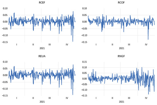
Figure 1.
Graph of the return data.
Table 2 presents the descriptive statistics and correlation structure for the variables. The average daily returns for all indices are positive but modest, ranging from 0.0003 (RCOF and RNGF) to 0.0007 (REUA), suggesting a generally stable upward trend over the sample period. However, the return distributions exhibit considerable asymmetry and fat tails, as evidenced by high kurtosis values, and the Jarque–Bera test results indicate that the data are not normally distributed. This non-normal behavior, coupled with the presence of volatility clustering confirmed by strong ARCH effects, with test statistics highly significant at the 1% level, indicates pronounced time-varying volatility.
Table 2.
Descriptive statistics and risk values.
The correlation matrix (Table 3) reveals that RCEF and REUA are almost perfectly correlated (0.9960), suggesting they may be tracking highly similar market segments or underlying assets. In contrast, RNGF exhibits weak correlations with the RCEF, implying potential diversification benefits when included in a broader clean energy portfolio.
Table 3.
Correlation coefficients.
The null hypothesis of a unit root is strongly rejected for all series. Table 4 indicates that each time series is stationary in levels, i.e., they are integrated of order zero, I(0). Therefore, no differencing is required for further time series modeling or analyses.
Table 4.
Unit root test results (ADF test).
4.2. Empirical Application
4.2.1. Conditional Value-at-Risk Approach
We initially compute the conditional value-at-risk (CVaR) at the 95% and 99% confidence levels, CVaR95 and CVaR99, respectively, to capture extreme downside risk in cryptocurrency portfolios. We then calculate the relative risk ratio (RRR) based on these values to assess the effect of clean cryptocurrencies’ tail risk mitigation.
Table 5 shows maximum profit and loss and VaR95, VaR99, CVaR95, and CVaR99 results for the variables. Regarding risk, RNGF stands out with the highest standard deviation and the most extreme daily return range, highlighting its relatively volatile nature. RCEF and REUA share identical extremes, while RCOF exhibits the narrowest range, suggesting a more stable profile.
Table 5.
Tail risk measures results.
Among the four assets, natural gas futures (RNGF) exhibits the most pronounced tail risk, with a VaR99 of −0.1656 and a CVaR99 of 0.0004. This indicates that under extreme market conditions, RNGF is subject to the most significant potential losses, consistent with its higher volatility profile. In contrast, crude oil futures (RCOF) demonstrates the lowest tail risk, with a VaR99 of −0.0699 and a CVaR99 of −0.0002, suggesting relatively more stable behavior in the left tail of the return distribution. Interestingly, the CVaR99 values for RCEF and REUA are slightly negative (−0.0005), implying that the expected loss beyond the 99% quantile is minimal but still present.
Figure 2 illustrates the changes in the relative risk ratio (RRR) for portfolios with increasing allocations of green assets as the weight of green assets increases by 0.05. The vertical axis shows the relative risk ratios, while the horizontal axis displays the weight of the green asset used in the calculation of RRR. For each RRR calculation, (see Equation (2)) starts from 1, while (see Equation (2)) is zero, and with each iteration, is decreased by 0.05 and is increased by 0.05, continuing until reaches 0 and reaches 1. Following Kuang (2025), the portfolio weights in 0.05 steps were incrementally adjusted to balance computational efficiency and analytical granularity. This step size was sufficient to capture the non-linear patterns in tail risk mitigation without introducing excessive noise or redundancy in the RRR curves.
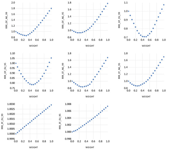
Figure 2.
Relative risk ratios. Note: RCOF, RCEF, REUA, and RNGF represent crude oil futures, carbon emissions futures, European Union Allowances, and natural gas futures, respectively; for brevity, these variables are abbreviated as OF, EF, EU, and NG, respectively. RRR_OF_NG_99: Relative risk ratio of return of crude oil futures and natural gas futures calculated by CVaR99 of the variables. The RRR_OF_NG_99 graph shows the RNGF weight. RRR_OF_NG_95: Relative risk ratio of return of crude oil futures and natural gas futures calculated by CVaR95 of the variables. The graphs can be interpreted in the same way as these two examples.
Portfolios incorporating natural gas output factors (RRR_OF_NG_99 and RRR_OF_NG_95) exhibit a clear monotonic increase in RRR values. Starting from a baseline of 1.0, both metrics rise steadily, reaching approximately 1.8 at full allocation. This trend suggests that increasing exposure to NG-based output factors significantly amplifies tail risk, particularly under extreme market conditions captured by CVaR99. The consistency across both confidence levels reinforces the robustness of this risk amplification effect.
In contrast, European output factors (RRR_OF_EU_99 and RRR_OF_EU_95) display a U-shaped trajectory. RRR values initially decline, reaching their lowest point around 40–50% allocation to green assets, before rising again toward the end of the spectrum. This pattern implies that moderate exposure to EU-based output factors may offer meaningful tail risk mitigation, especially under CVaR95, while excessive allocation could reverse these benefits. The presence of a turning point highlights the importance of identifying optimal thresholds for diversification.
A similar U-shaped behavior can be observed for natural gas emissions factors (RRR_EF_NG_99 and RRR_EF_NG_95). The tail risk decreases during the initial phase of green asset integration but begins to rise sharply beyond the 40% allocation mark. This suggests that NG-based emission factors may provide diversification benefits at low to moderate levels yet contribute to increased risk when their portfolio share becomes dominant. The steepness of the upward slope in the latter half of the curve signals a potential risk concentration effect.
Meanwhile, European emissions factors (RRR_EF_EU_99 and RRR_EF_EU_95) exhibit a subtle but consistent upward trend. Although the increase in RRR is marginal, it indicates that higher allocations to EU-based emission factors may incrementally elevate tail risk. The linearity of this trend suggests a predictable risk profile, which may be advantageous for portfolio managers seeking stability.
Taken together, these findings highlight the non-linear and heterogeneous nature of tail risk responses to green asset integration. The coexistence of monotonic and U-shaped patterns across different asset classes and risk thresholds underscores the need for nuanced portfolio construction strategies. Optimal allocation is not merely a function of environmental preference but also a critical determinant of financial resilience under stress scenarios. By focusing on quantile thresholds (q10, q5, q1) using daily data from 1 April 2021 to 25 June 2025, we ensure that our results capture genuine ‘extreme market downturns’—including the post-COVID rebound and the 2022–2023 energy crisis volatility—thereby grounding economic significance in real stress episodes. Although no broad systemic crash occurred during our sample, the very severe tail events isolated via the lowest 1% and 5% CVaR scenarios serve as de facto crisis-like conditions, demonstrating that our monotonic and U-shaped risk patterns remain economically material.
4.2.2. Dynamic Conditional Correlation Approach
Based on the unit root results, the integration level is I(0); therefore, the ARIMA model is not used, and the ARMA model is applied. The ARMA (0,0) model is selected, and for the GARCH model, the GARCH(1,1) model is chosen. DCC model results are presented in Table 6.
Table 6.
DCC model results.
The DCC coefficients (ρ) are positive and significant at the 1% level, except the DCC_RCEF_RNGF model. Across the four DCC models estimated, three exhibit statistically significant α and β coefficients with their sums remaining below unity, indicating stable and mean-reverting conditional correlations. These include the RCEF–REUA, RCEF–RNGF, and RCOF–RNGF models. In contrast, the RCOF–REUA model presents an insignificant α coefficient, although the β term is significant and the sum of both parameters remains below one. This suggests that while the model is statistically stable, its responsiveness to new information is limited. Notably, similar evidence of insignificant α parameters has been reported by Kamal et al. (2024), who interpret this as indicative of the absence of short-run volatility clustering. Consistent with their approach, although some α coefficients here are not statistically significant, we retain the DCC specification rather than reverting to a constant conditional correlation (CCC) model. This choice is motivated by our primary objective to assess the safe haven properties of these assets through their time-varying dependence with uncertainty indices.
The diagnostic statistics generally support the adequacy of the DCC-GARCH specification. For most models, the Hosking and Li–McLeod multivariate portmanteau tests on standardized residuals and squared standardized residuals yield p-values well above the 5% threshold, suggesting no evidence of remaining serial correlation or ARCH effects. The notable exception is the DCC_RCOF_RNGF model, where Q(5) and Q(10) statistics for null hypotheses are rejected, indicating some degree of autocorrelation that could be addressed in future refinements.
Overall, these findings reveal heterogeneous dependence structures across the examined pairs, highlighting both substantial long-run correlation persistence, and in some cases limited sensitivity to short-term innovations. These patterns are particularly relevant for portfolio diversification, hedging strategies, and the assessment of safe haven characteristics under varying market conditions.
The calculated DCC coefficients are presented in Figure 3.
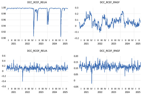
Figure 3.
DCC coefficients of the DCC-GARCH model.
The dynamic conditional correlation (DCC) analysis between carbon and energy futures from 2021 to 2025 reveals distinct temporal patterns across asset pairings. The correlation between carbon emissions futures and EUA futures (DCC_RCEF_REUA) remains consistently high, fluctuating narrowly around 0.99, which indicates a stable and strong positive relationship. However, noticeable declines can be observed in early 2023 and early 2024. In contrast, the correlation between carbon emissions futures and natural gas futures (DCC_RCEF_RNGF) exhibits substantial volatility. Peaks happen around the middle of 2022 and 2024, and lows can be seen in early 2023 and late 2024. This shows that the situation is changing and unpredictable. The relationship between crude oil futures and EUA futures (DCC_RCOF_REUA) fluctuates within a moderate band, with a significant drop in early 2023, indicating episodic divergence. Lastly, the correlation between crude oil futures and natural gas futures (DCC_RCOF_RNGF) remains relatively stable, with values ranging from −0.05 to +0.20, suggesting a consistent co-movement throughout the sample period. Collectively, these patterns underscore the differing levels of integration and responsiveness among carbon and energy derivatives, with EUA futures demonstrating the most stable correlation and natural gas futures exhibiting the greatest volatility.
The main aim of this article is to investigate the hedge and safe haven properties of green assets against dirt assets. To test these properties, we use hedge and safe haven regression tests. Table 7 shows the model results.
Table 7.
Hedge and safe haven analyses.
Table 7 reports selected asset pairs’ hedge and safe haven properties under extreme market conditions. The hedge coefficients (θ0) are statistically significant across all pairs, indicating that the examined assets exhibit a consistent co-movement in normal market conditions. However, the magnitude of these coefficients varies considerably. For instance, the RCEF_REUA pair shows a high relationship, suggesting a lack of hedging potential, whereas RCEF_RNGF displays a much lower coefficient, implying a weak relationship. In contrast, the safe haven coefficients (θ1, θ2, θ3), which capture asset behavior during the 10%, 5%, and 1% lower quantiles of returns, are largely statistically insignificant across all pairs. This means that green assets do not act as safe havens against dirty assets, as their behavior during extreme market downturns is not statistically different from normal conditions.
5. Discussion and Conclusions
Among the investigated futures, natural gas stands out as the most volatile, displaying the widest range of daily returns and the most significant exposure to extreme losses. Its sensitivity to market shocks underscores the importance of cautious allocation. In contrast, crude oil futures demonstrate more stable behavior with relatively limited downside risk. While less volatile than natural gas, renewable energy ETFs still carry minor tail risk, suggesting their defensive qualities might be limited during severe stress. These findings emphasize the critical role of asset selection in managing downside risk within energy-focused portfolios.
A further analysis of the risk ratios highlights the complex relationship between clean and dirty assets. This non-linear relationship underscores the importance of optimal allocation strategies when combining environmentally sustainable assets with more volatile, energy-intensive ones. Conversely, some clean assets exhibit a U-shaped risk profile, initially reducing tail risk at low allocations but increasing it beyond a certain threshold.
The DCC analysis demonstrates meaningful time-varying relationships among asset pairs. Most models show statistically significant, stable correlation dynamics, suggesting that conditional correlations tend to be mean-reverting and responsive to market conditions. Although limited short-term volatility transmission can be observed in some cases, the DCC framework effectively captures evolving dependence structures, especially when assessing safe haven behavior under uncertainty. These results are consistent with findings by Ren and Lucey (2022b), who discovered predominantly positive, yet relatively low, dynamic conditional correlations between clean energy indices and dirty and clean cryptocurrencies, implying limited hedging potential. Similarly, Ali et al. (2024) found that green cryptocurrency correlations with equity indices are generally lower and more diverse than those of non-green cryptocurrencies, indicating better diversification prospects under normal conditions.
In light of the findings, H1 is not supported, as green assets do not consistently exhibit safe haven behavior under stress. However, H2 is partially confirmed, with tail risk mitigation observed when green asset weights exceed 40%, particularly for natural gas futures. These results underscore the conditional utility of green assets in portfolio risk management.
Finally, the hedge and safe haven analysis provides key insights into the interaction between green and dirty assets. Statistically significant hedge coefficients suggest co-movement under typical market conditions, but largely insignificant safe haven coefficients imply that green assets offer limited protection during extreme downturns, although some may mitigate tail risk when their portfolio weight exceeds 40%. This challenges the notion that environmentally sustainable assets inherently act as effective defensive tools. Instead, the data suggest they contribute to diversification in stable periods but tend to decouple during stressed market phases. Kuang (2025) supports this view, finding insignificant safe haven coefficients for clean cryptocurrencies, which indicates limited protection during downturns. Ren and Lucey (2022b) observe similar patterns with clean energy indices, and Ali et al. (2024) report that green and non-green cryptocurrencies generally do not serve as strong safe havens during market stress, as their coefficients at extreme quantiles largely lack significance. In contrast, Bredin et al. (2017) note that while precious metals like gold can reduce downside risk in the short term, they do not consistently function as safe havens in the long run, often sacrificing risk-adjusted returns for protection.
This study highlights the complex and evolving dynamics between clean and dirty energy assets in portfolio construction. While certain clean assets can reduce tail risk beyond specific allocation thresholds, their effectiveness as safe havens remains limited, particularly during periods of extreme market stress. The non-linear patterns observed in relative risk ratios and time-varying correlations captured through the DCC analysis emphasize the importance of strategic asset allocation and continuous risk monitoring. Overall, the findings challenge simplistic assumptions about asset defensiveness and underscore the need for data-driven approaches to managing risk in energy-focused portfolios.
While green assets are often perceived as defensive due to their ESG profile, our findings suggest that structural factors undermine their safe haven potential. Regulatory shocks—such as abrupt changes in carbon pricing or subsidy schemes—can trigger volatility in green markets. Illiquidity in green futures, especially during stress periods, amplifies price swings. Moreover, macroeconomic co-movement with broader energy indices reduces their decoupling capacity. Rather than investor sentiment alone, these structural dynamics explain why green assets consistently fail to act as safe havens.
These findings suggest that while certain green assets may offer protection against extreme downside risk, particularly in the lower tail of the return distribution, they do not consistently exhibit the negative correlation or crisis resilience typically associated with safe haven assets. This distinction underscores the nuanced role of green assets in portfolio risk management and highlights the importance of separating tail risk mitigation from broader safe haven behavior.
The observed tail risk mitigation effects suggest that while not serving as traditional safe havens, green assets can still act as effective downside buffers in diversified portfolios, especially when allocated within certain threshold ranges. These findings highlight the need for developing regulatory frameworks that acknowledge the risk of mitigating the potential of green financial instruments, even if they do not meet strict safe haven standards. Tail risk resilience could be a useful additional metric in green finance assessments. Portfolio construction strategies aiming to align environmental goals with risk management might benefit from including green assets not for their safe haven status but for their conditional tail risk behavior. Optimization models could be adjusted to account for this nuanced approach.
For further robustness, future extensions could apply the same quantile-based framework to the pre-2008 and 2020 COVID crisis periods, testing whether the economic significance of our RRR dynamics persists across multiple market shock regimes. Policy-makers designing carbon and energy markets may benefit from incorporating liquidity buffers and dynamic regulatory thresholds to avoid abrupt regime shifts that destabilize green asset behavior.
Funding
This research received no external funding.
Data Availability Statement
The original data presented in the study are openly available in Zenodo at DOI https://doi.org/10.5281/zenodo.15802492 (accessed on 3 July 2025).
Conflicts of Interest
The author declares no conflicts of interest.
References
- Ali, Fahad, Muhammad Usman Khurram, Ahmet Sensoy, and Xuan Vinh Vo. 2024. Green Cryptocurrencies and Portfolio Diversification in the Era of Greener Paths. Renewable and Sustainable Energy Reviews 191: 114137. [Google Scholar] [CrossRef]
- Baur, Dirk G., and Brian M. Lucey. 2010. Is Gold a Hedge or a Safe Haven? An Analysis of Stocks, Bonds and Gold. Financial Review 45: 217–29. [Google Scholar] [CrossRef]
- Baur, Dirk G., and Thomas K. McDermott. 2010. Is Gold a Safe Haven? International Evidence. Journal of Banking & Finance 34: 1886–98. [Google Scholar] [CrossRef]
- Bredin, Don, Thomas Conlon, and Valerio Potì. 2017. The Price of Shelter—Downside Risk Reduction with Precious Metals. International Review of Financial Analysis 49: 48–58. [Google Scholar] [CrossRef]
- Bunnag, Tanattrin. 2015. Volatility Transmission in Oil Futures Markets and Carbon Emissions Futures. International Journal of Energy Economics and Policy 5: 3. [Google Scholar]
- Conrad, Christian, Daniel Rittler, and Waldemar Rotfuß. 2012. Modeling and Explaining the Dynamics of European Union Allowance Prices at High-Frequency. Energy Economics 34: 316–26. [Google Scholar] [CrossRef]
- Cornish, Edmund A., and Ronald A. Fisher. 1938. Moments and Cumulants in the Specification of Distributions. Revue de l’Institut International de Statistique/Review of the International Statistical Institute 5: 307–20. [Google Scholar] [CrossRef]
- Dias, Rui, Paulo Alexandre, Nuno Teixeira, and Mariana Chambino. 2023. Clean Energy Stocks: Resilient Safe Havens in the Volatility of Dirty Cryptocurrencies. Energies 16: 5232. [Google Scholar] [CrossRef]
- Economides, Michael J., and David A. Wood. 2009. The State of Natural Gas. Journal of Natural Gas Science and Engineering 1: 1–13. [Google Scholar] [CrossRef]
- Elie, Bouri, Jalkh Naji, Anupam Dutta, and Gazi Salah Uddin. 2019. Gold and Crude Oil as Safe-Haven Assets for Clean Energy Stock Indices: Blended Copulas Approach. Energy 178: 544–53. [Google Scholar] [CrossRef]
- Gülen, S. Gürcan. 1998. Efficiency in the Crude Oil Futures Market. Journal of Energy Finance & Development 3: 13–21. [Google Scholar] [CrossRef]
- Hoque, Mohammad Enamul, and Sourav Batabyal. 2022. Carbon Futures and Clean Energy Stocks: Do They Hedge or Safe Haven against the Climate Policy Uncertainty? Journal of Risk and Financial Management 15: 397. [Google Scholar] [CrossRef]
- Hoque, Mohammad Enamul, Faik Bilgili, and Sourav Batabyal. 2023. What Do We Know about Spillover between the Climate Change Futures Market and the Carbon Futures Market? Climatic Change 176: 166. [Google Scholar] [CrossRef]
- Howarth, Robert W., Renee Santoro, and Anthony Ingraffea. 2011. Methane and the Greenhouse-Gas Footprint of Natural Gas from Shale Formations. Climatic Change 106: 679–90. [Google Scholar] [CrossRef]
- Huang, Jie, Yu Cao, and Pengshu Zhong. 2022. Searching for a Safe Haven to Crude Oil: Green Bond or Precious Metals? Finance Research Letters 50: 103303. [Google Scholar] [CrossRef]
- IEA. 2019. Demand from Asia Is Set to Power the Growth of the Global Gas Industry over the Next Five Years—News. IEA. June 7. Available online: https://www.iea.org/news/demand-from-asia-is-set-to-power-the-growth-of-the-global-gas-industry-over-the-next-five-years (accessed on 27 May 2025).
- Kamal, Javed Bin, Mark Wohar, and Khaled Bin Kamal. 2024. On the Potential Hedging Instruments Against Central Bank Digital Currency Uncertainty and Attention Indices. Asian Economics Letters 5. [Google Scholar] [CrossRef]
- Kuang, Wei. 2021. Are Clean Energy Assets a Safe Haven for International Equity Markets? Journal of Cleaner Production 302: 127006. [Google Scholar] [CrossRef]
- Kuang, Wei. 2025. Greening Crypto Portfolios: The Diversification and Safe Haven Potential of Clean Cryptocurrencies. Humanities and Social Sciences Communications 12: 850. [Google Scholar] [CrossRef]
- Li, Jiaman, Xiucheng Dong, and Kangyin Dong. 2022. Green Efficiency of Natural Gas and Driving Factors Analysis: The Role of the Natural Gas Price in China. Energy Efficiency 15: 24. [Google Scholar] [CrossRef]
- Liu, Changyu, Muhammad Abubakr Naeem, Mobeen Ur Rehman, Saqib Farid, and Syed Jawad Hussain Shahzad. 2020. Oil as Hedge, Safe-Haven, and Diversifier for Conventional Currencies. Energies 13: 4354. [Google Scholar] [CrossRef]
- Markowitz, Harry. 1952. Portfolio Selection. The Journal of Finance 7: 77–91. [Google Scholar] [CrossRef]
- Ming, Lei, Ping Yang, Xinyi Tian, Shenggang Yang, and Minyi Dong. 2023. Safe Haven for Crude Oil: Gold or Currencies? Finance Research Letters 54: 103793. [Google Scholar] [CrossRef]
- Pacala, Stephen, and Robert Socolow. 2004. Stabilization Wedges: Solving the Climate Problem for the Next 50 Years with Current Technologies. Science 305: 968–72. [Google Scholar] [CrossRef] [PubMed]
- Reboredo, Juan C. 2013. Modeling EU Allowances and Oil Market Interdependence. Implications for Portfolio Management. Energy Economics 36: 471–80. [Google Scholar] [CrossRef]
- Ren, Boru, and Brian Lucey. 2022a. A Clean, Green Haven?—Examining the Relationship between Clean Energy, Clean and Dirty Cryptocurrencies. Energy Economics 109: 105951. [Google Scholar] [CrossRef]
- Ren, Boru, and Brian Lucey. 2022b. Do Clean and Dirty Cryptocurrency Markets Herd Differently? Finance Research Letters 47: 102795. [Google Scholar] [CrossRef]
- Shaton, Katerina, Arild Hervik, and Harald M. Hjelle. 2020. The Environmental Footprint of Natural Gas Transportation: LNG vs. Pipeline. Economics of Energy & Environmental Policy 9: 223–42. [Google Scholar] [CrossRef]
- Sterner, Thomas. 2024. Carbon Pricing Reduces Emissions. Nature 632: 31–32. [Google Scholar] [CrossRef]
- Sun, Chuanwang, Yanhong Zhan, Yiqi Peng, and Weiyi Cai. 2022. Crude Oil Price and Exchange Rate: Evidence from the Period before and after the Launch of China’s Crude Oil Futures. Energy Economics 105: 105707. [Google Scholar] [CrossRef]
- Tian, Hong-Zhi, and Wei-Di Lai. 2019. The Causes of Stage Expansion of WTI/Brent Spread. Petroleum Science 16: 1493–505. [Google Scholar] [CrossRef]
- UNFCCC. n.d. The Collaborative Instruments for Ambitious Climate Action (CiACA): About Carbon Pricing. Available online: https://unfccc.int/about-us/regional-collaboration-centres/the-ciaca/about-carbon-pricing (accessed on 6 June 2025).
- Wei, Ching-chun, and Ya-g Lin. 2016. Carbon Future Price Return, Oil Future Price Return and Stock Index Future Price Return in the U.S. International Journal of Energy Economics and Policy 6: 655–62. [Google Scholar]
- Zhang, Wenting, Xie He, Tadahiro Nakajima, and Shigeyuki Hamori. 2020. How Does the Spillover among Natural Gas, Crude Oil, and Electricity Utility Stocks Change over Time? Evidence from North America and Europe. Energies 13: 727. [Google Scholar] [CrossRef]


Disclaimer/Publisher’s Note: The statements, opinions and data contained in all publications are solely those of the individual author(s) and contributor(s) and not of MDPI and/or the editor(s). MDPI and/or the editor(s) disclaim responsibility for any injury to people or property resulting from any ideas, methods, instructions or products referred to in the content. |
© 2025 by the author. Licensee MDPI, Basel, Switzerland. This article is an open access article distributed under the terms and conditions of the Creative Commons Attribution (CC BY) license (https://creativecommons.org/licenses/by/4.0/).