Article

Survival Analysis for Credit Risk: A Dynamic Approach for Basel IRB Compliance

by
Fernando L. Dala
1,
Manuel L. Esquível
2 and
Raquel M. Gaspar
3,*
1
Banco Nacional de Angola, Av. 4 de Fevereiro n. 151, Luanda, Angola
2
School of Science and Technology and Nova Math, Universidade Nova de Lisboa, 2829-516 Caparica, Portugal
3
ISEG Research, Lisbon School of Economics and Management, Universidade de Lisboa, Rua do Quelhas, n. 6, 1200-781 Lisboa, Portugal
*
Author to whom correspondence should be addressed.
Risks 2025, 13(8), 155; https://doi.org/10.3390/risks13080155
Submission received: 23 June 2025 / Revised: 21 July 2025 / Accepted: 5 August 2025 / Published: 15 August 2025
(This article belongs to the Special Issue Advances in Risk Models and Actuarial Science)

Abstract

This paper uses survival analysis as a tool to assess credit risk in loan portfolios within the framework of the Basel Internal Ratings-Based (IRB) approach. By modeling the time to default using survival functions, the methodology allows for the estimation of default probabilities and the dynamic evaluation of portfolio performance. The model explicitly accounts for right censoring and demonstrates strong predictive accuracy. Furthermore, by incorporating additional information about the portfolio’s loss process, we show how to empirically estimate key risk measures—such as Value at Risk (VaR) and Expected Shortfall (ES)—that are sensitive to the age of the loans. Through simulations, we illustrate how loss distributions and the corresponding risk measures evolve over the loans’ life cycles. Our approach emphasizes the significant dependence of risk metrics on loan age, illustrating that risk profiles are inherently dynamic rather than static. Using a real-world dataset of 10,479 loans issued by Angolan commercial banks, combined with assumptions regarding loss processes, we demonstrate the practical applicability of the proposed methodology. This approach is particularly relevant for emerging markets with limited access to advanced credit risk modeling infrastructure.

1. Introduction

Survival analysis—a statistical methodology traditionally used in actuarial science, healthcare, engineering, and reliability studies—has seen growing relevance in the financial sector (Kleinbaum and Klein 2012b). In particular, it offers a robust framework for modeling time-to-event data, such as the time until a loan defaults. This temporal dimension makes survival analysis especially suitable for assessing credit risk in loan portfolios, aligning with the Internal Ratings-Based (IRB) approach under the Basel regulatory framework (BIS 2006).
Unlike traditional credit scoring models that offer static default probabilities, survival analysis enables a dynamic, time-dependent understanding of credit risk. By modeling the time to default, financial institutions can obtain more detailed insights into when defaults are likely to occur, thereby enhancing their ability to manage risk exposure, allocate capital efficiently, and comply with regulatory requirements.
This paper presents a survival analysis-based methodology for estimating default probabilities and assessing credit risk in loan portfolios. We employ the Gompertz–Makeham parametric model to characterize the time to default, explicitly incorporating right-censored observations, which are common in loan data. These occur when the default event is not observed within the observation window—for example, due to early repayment, transfer to another institution, or loan maturity. Right censoring requires special attention during estimation, as it limits the available information on the timing of potential defaults. Properly accounting for censored data is essential to avoid biased estimates of default intensities and survival probabilities.
Survival analysis offers several practical advantages for credit risk management:
  • Granular Risk Profiling: It enables the evaluation of credit risk at the level of individual loans or borrower segments.
  • Dynamic Monitoring: Time-based risk assessment supports early detection of deteriorating credit quality.
  • Strategic Insights: Outputs from survival models inform pricing, capital provisioning, and portfolio allocation decisions.
  • Regulatory Alignment: The methodology supports key requirements of the IRB approach within the Basel framework (BCBS 2011).
In implementing this approach, we use a dataset of 10,479 loans from Angolan commercial banks. The dataset includes detailed information on loan characteristics, payment histories, and the timing of default or prepayment. Based on this information, we estimate survival functions and compute hazard ratios that reflect the relative risk of default over time. Unfortunately, the database does not contain direct information on losses. However, we show how the model can be easily extended to incorporate a calibration of loss given default (LGD), allowing for the construction of a complete loss process. This extension enables the estimation of key risk metrics such as Value at Risk (VaR) and Expected Shortfall (ES). In addition, we propose a novel approach to estimate VaR and ES as a function of loan age, providing a dynamic view of credit risk throughout the life cycle of a loan.
The remainder of the paper is organized as follows. Section 2 presents a concise review of the literature on credit risk assessment in loan portfolios. Section 3 introduces the survival analysis framework, outlining the key variables and methodological foundations. Section 4 details our empirical application using loan-level data from Angolan banks. This section is structured to highlight each stage of the methodological approach, demonstrating how to model loss given default (LGD) in conjunction with default probabilities to construct realistic loss processes. It concludes by illustrating how the framework can be used to analyze the evolving risk profile of loan portfolios and derive risk measures by loan age. Finally, Section 6 summarizes the main findings and discusses their implications for credit risk management.

2. Literature Review

Credit risk modeling has evolved significantly, with methodologies ranging from traditional statistical techniques to advanced machine learning (ML) and survival analysis. Early approaches, such as those by Micocci (2000), relied on Monte Carlo simulations to estimate default rates, while Crosbie and Bohn (2003) combined accounting- and market-based indicators to calibrate default probabilities. These foundational works, however, often made simplifying assumptions (e.g., static transition matrices, constant interest rates) that limited their adaptability to dynamic economic environments (Derbali 2018).
Macroeconomic drivers of credit risk have been extensively studied, particularly in emerging markets. For instance, Poudel (2013) demonstrated the impact of economic variables on credit risk in Nepal, highlighting macro-financial linkages. Structural and reduced-form models, such as those by Suisse (1997) and Zokirjonov (2018), extended credit risk assessment to include rating migrations and portfolio-level Value at Risk (VaR). Yet, these models often struggle with high-dimensional, non-linear data—a gap that ML methods have sought to address. Recent work by Bo (2024) underscores how macroeconomic shocks amplify model risk in regulatory frameworks in developing countries’ baks.
The advancement of machine learning has introduced powerful alternatives for credit risk modeling (Leo et al. 2019). ML techniques, such as ensemble learning (Charpignon et al. 2014) and deep neural networks (Mahbobi et al. 2023), excel at capturing complex patterns in large datasets. Recent studies, like Sharma et al. (2022) or Hernes et al. (2023), show that ML models (e.g., XGBoost, random forests) often outperform traditional logistic regression in default prediction due to their ability to handle non-linear interactions. Cutting-edge ML approaches continue to push boundaries. Huang et al. (2025) apply language learning to small- and medium-sized enterprises (SMEs) credit risk, achieving superior accuracy but underscoring computational costs. Meanwhile, Kakadiya et al. (2024) leverage transformer architectures for default prediction, demonstrating state-of-the-art performance in high-data environments. However, their effectiveness depends heavily on data quality and volume, posing challenges for banks in emerging markets or smaller institutions with limited data infrastructure (Fejza et al. 2022). Additionally, ML models are often criticized as “black boxes,” lacking interpretability—a key requirement for regulatory compliance under frameworks like Basel IRB (Erkkilä 2025; Hurlin and Pérignon 2023).
Amid these developments, survival analysis has emerged as a particularly suitable approach for modeling credit risk in a time-sensitive and probabilistic framework. Originally applied in biomedical and reliability studies, survival models are increasingly being adopted in credit scoring and default prediction due to their ability to handle censored observations and time-varying covariates. Banasik et al. (1999) and Stepanova and Thomas (2002) were among the first to apply survival techniques to consumer credit, enabling a more granular analysis of default timing. McDonald et al. (2010) combine survival analysis with Monte Carlo simulation to price mortgages and forecast cash flow distributions. Likewise, Hassan et al. (2018) use accelerated failure time models to estimate both the probability and timing of default, incorporating borrower characteristics and macroeconomic indicators. Recent advances in survival analysis have focused on addressing real-world constraints in credit risk modeling. Zhang et al. (2021) developed DeepSurv for corporate default prediction, demonstrating how neural networks can enhance traditional Cox models while maintaining interpretability. For federated learning applications—particularly relevant for multi-institutional risk modeling—Kragh Jørgensen et al. (2025) established foundational methods for discrete-time Cox models which can be applied in privacy-preserving environments, though implementation challenges remain for real-time banking applications. These studies focus on modeling the default event, but lack its connection to losses and risk measure, which is key in addressing the existent regulatory framework.
The choice between survival analysis and ML depends on the use case. While ML excels in high-data environments (e.g., Borisov et al. (2022)), survival analysis is more adaptable to sparse datasets and provides explicit time-to-event estimates—critical for regulatory capital calculations under IRB. On the data scarcity and the limitations of ML, see for instance Abdalla et al. (2025). Hybrid approaches are emerging as promising solutions (Baesens et al. 2005). For instance, Siphuma and van Zyl (2025) introduced Transformer survival models for credit risk, achieving state-of-the-art performance in temporal pattern recognition while Djeundje and Crook (2019) developed dynamic survival analysis frameworks specifically for loan portfolios. These approaches address the critical need for models that adapt to evolving economic conditions, a key requirement under Basel III, but also depend on large datasets, which are not available in emerging markets.
The choice between survival analysis and ML thus depends on the use case. While ML excels in high-data environments (e.g., Borisov et al. (2022)), survival analysis is more adaptable to sparse datasets and provides explicit time-to-event estimates—critical for regulatory capital calculations under IRB. On the data scarcity and the limitations of ML, see for instance Abdalla et al. (2025).
We propose a survival-based framework for IRB compliance, emphasizing not only time-to-default estimation, but also dynamic risk metrics (e.g., age-dependent VaR and ES). Unlike ML models, our approach is data-efficient and interpretable, making it suitable for banks with limited data. We extend survival analysis to loss given default (LGD) modeling, enabling end-to-end loss process simulation. In opposition to the existent literature we illustrate our approach on real data from a set of Angolan banks, thus focusing on the difficulties faced by emerging markets’ banks.

3. Survival Analysis

Survival analysis is a statistical method used to analyze time-to-event data, where the event of interest—such as failure, recovery, or death—can occur at any point in time. Its primary objective is to estimate the likelihood of the event occurring over time. A key challenge in survival analysis is dealing with right-censored data, where the exact timing of the event is unknown for some observations, but it is known that the event has not occurred up to a certain point.
This modeling framework is particularly relevant for credit risk analysis, where we may observe defaults, but we may also observe loan repayment (at maturity), early settlement, or transfer to another institution —situations that lead to right-censored data.
In what follows, we introduce the survival analysis method, establish the key notation, and demonstrate its application to a credit portfolio. Most of the theoretical foundations are drawn from actuarial references such as Rocha and Papoila (2009), Kleinbaum and Klein (2012a), Dickson et al. (2013), and Smith (2017).

3.1. Setup and Notation

Let us define the “lifetime of a loan” as a non-negative, real-valued random variable T, representing the duration from loan origination to either default or censoring.
Based on the random variable T, we define the following:
  • Age of a loan t: The duration (in years) from the origination date until default or the end of the observation period, where t 0 .
  • Loan at age t: Denoted as ( t ) .
  • Maturity of a loan M: The time at which the loan is contractually scheduled to end.
  • Remaining lifetime of a loan T t : The time left until default or maturity, satisfying 0 t + T M .
  • At the loan’s origination ( t = 0 ), we have T = 0 .
The survival distribution function  S ( t ) is the probability that a loan survives longer than time t, mathematically expressed as:
S ( t ) = P ( T > t ) = 1 F ( t ) ,
where F ( t ) is the cumulative distribution function (CDF) of T, representing the probability of default by time t. Denoted by f ( t ) the probability density function (pdf) of F ( t ) , it follows that f ( t ) = d S ( t ) d t .
The hazard rate function, h ( t ) , focuses on the instantaneous probability of default. For a loan that has survived until time t (i.e., T > t ), the conditional probability of default in the next small interval ( t , t + d t ) is given by the following:
h ( t ) = lim d t 0 P r ( t T t + d t | T > t ) d t = f ( t ) S ( t ) = t log [ S ( t ) ] .
Since h ( t ) is derived from a probability density function, it satisfies h ( t ) 0 . However, because h ( t ) is not itself a probability, it is not necessarily less than 1. For very small d t , we can interpret h ( t ) d t as the approximate probability that a loan, having reached age t, defaults before reaching age t + d t :
h ( t ) d t P ( T t + d t | T > t ) .
Rearranging Equation (2), we get
S ( t ) = exp 0 t h ( u ) d u = exp [ H ( t ) ] ,
where the cumulative hazard function H ( t ) is defined as
H ( t ) = 0 t h ( u ) d u .
Also from Equation (2), the density function f ( t ) can then be written in terms of S ( t ) and h ( t ) ,
f ( t ) = S ( t ) h ( t ) .
Considering N ( t ) the number of defaults at risk at time t, the expected number of defaults at time t, d ( t ) , is given by
d ( t ) = N ( t ) f ( t ) .

3.2. Censoring

As previously mentioned, in the context of loan portfolios, censoring occurs when a loan is repaid in full before its scheduled term, transferred to another financial institution with due compensation to the original lender or reaches its contractual maturity M without defaulting. For those observations, the exact time of default is unknown and is treated as right-censored. Figure 1 illustrates instances of censored data. Right censorship leads to special care when building the key estimates for the survival table, in the next section.
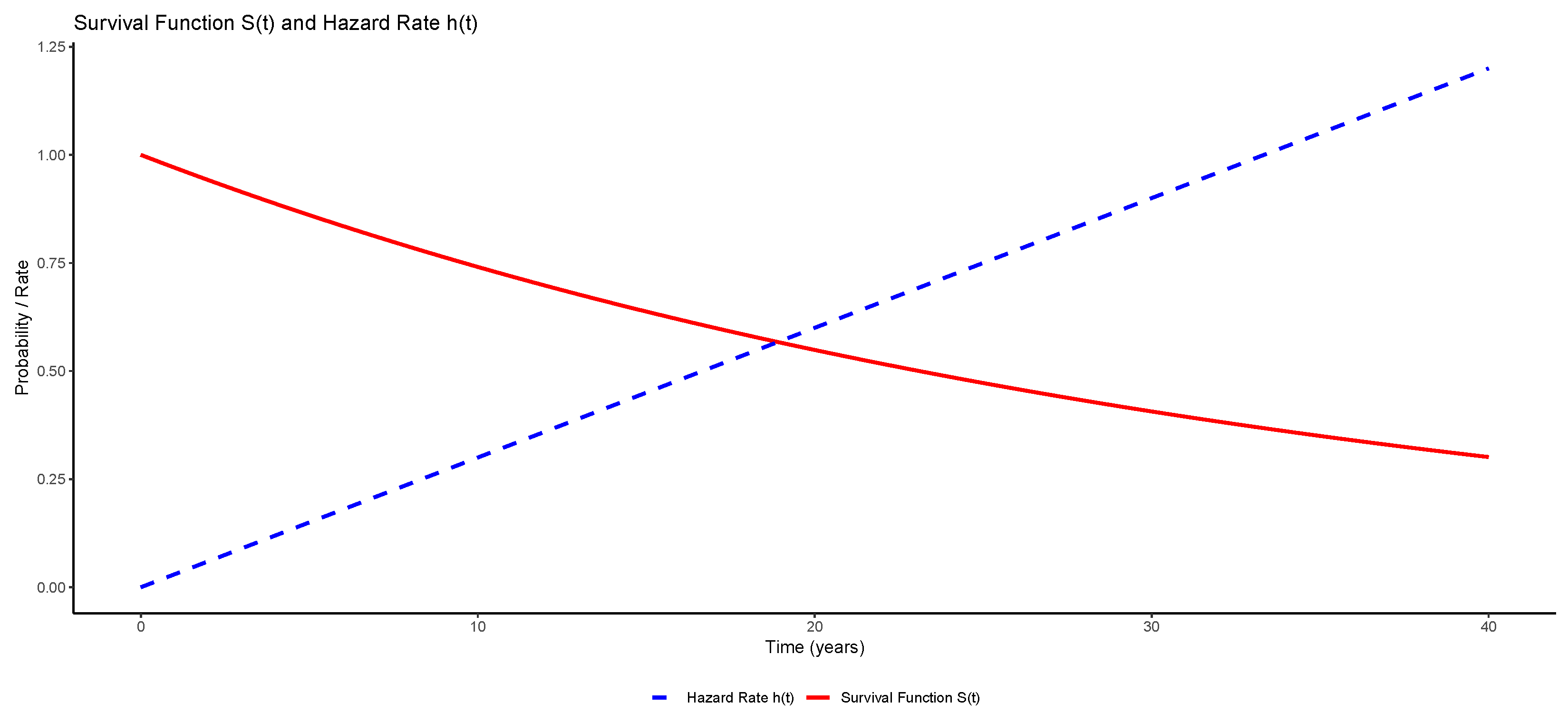
Using data from our empirical study, Figure 2 illustrates the relationship between the survival function S ( t ) and the hazard rate function h ( t ) over time, with right censoring already considered. As time progresses, the survival probability S ( t ) (red line) decreases, while the hazard rate h ( t ) (red dashed line) increases, representing the growing risk of default as loans age.
When determining the number of defaults in a censored dataset, the survival function S ( t ) is derived from the number of loans at risk (still “alive”). Therefore, defaults should be calculated relative to the remaining loan pool, N ( t ) at each t.

3.3. Survival Table

Consider a cohort of n loans from a given portfolio. The interval [ 0 , ) is divided into k + 1 adjacent intervals of fixed width,
I j = [ t j 1 , t j ) , j = 1 , , k + 1 ,
with t 0 = 0 , t k = M , and t k + 1 = , where M is the upper limit of observation.
The data consists of the number of loans active at the beginning of each interval and the number of loans that defaulted or are censored in each interval.
Let us denote
  • n j : number of loans at risk at the beginning of interval I j ;
  • d j : number of defaults observed in I j ;
  • m j : number of censored observations in I j .
With these we determine the number of loans at risk at the beginning of interval I j as
n j = n j 1 d j 1 m j 1 for j = 2 , 3 , , k + 1 .
The Kaplan and Meier (1958) estimator is a non-parametric method for estimating the survival function S ( t ) , accounting for right-censored data. The estimator computes the probability of surviving beyond each observed time point. If we had complete data, we could simply calculate the fraction of survivors at each time step. However, right-censored observations introduce uncertainty, so we need to adjust accordingly.
Instead of treating censored cases as failures, we only consider observed default events when updating survival probabilities. At each time t where a default occurs, we update the survival function based on the fraction of loans still “at risk” (i.e., not defaulted or censored before).
To estimate the survival function S ( t ) , we start by determining the estimated probability of default in the interval I j . This can be calculated using the actuarial estimator,
q ^ j = d j n j m j 2 for n j > 0 ,
where q ^ j is the estimated probability of default in interval I j , adjusted for censoring (Rocha and Papoila 2009). Here, d j represents the number of defaults, n j is the number of loans at the beginning of the interval, and m j denotes the number of censored observations in interval I j .
Note that n j m j 2 is the adjusted number of loans at risk in interval I j . The adjustment is crucial for accurately estimating the number of loans at risk within interval I j in the presence of censoring. The adjustment n j m j 2 assumes that the instances of censoring are uniformly distributed throughout the interval I j .
The estimated probability of survival through interval I j is then as follows:
s ^ j = 1 q ^ j ,
and the cumulative survival probability S ^ j up to the end of interval I j is given by the following:
S ^ j = i = 1 j s ^ i .
Alternatively, it can be expressed recursively as S ^ j = s ^ j · S ^ j 1 , with S ^ 0 = 1 .

4. Empirical Application

In this section, we present an application of survival analysis to a portfolio of loans, demonstrating its practical use in evaluating credit risk.
The analysis is based on a dataset of 10,479 loans from the portfolios of 10 Angolan commercial banks, all classified within the same rating category and all with the same maturity of 40 years. The observation period spans from the origination date of each loan to the occurrence of a default or the end of the observation period. The latter includes scenarios where loans reach maturity, are prepaid, or are transferred to another financial institution with due compensation to the original lender.
Table 1 gives a detailed statistical overview of loan defaults and survival rates over their lifetime. Its columns are as follows: age (in years), for each interval, d j shows the number of defaults, m j shows the number of censored loans, and n j shows the number of credits at risk in the beginning of the interval. The remaining columns result from the above formulas; q ^ j is the estimated default probability in the interval (Equation (8)), s ^ j the estimated survival probability in the interval (Equation (9)), and S ^ j represents the estimated cumulative survival probability (Equation (10)).
From Table 1, we observe that the estimated cumulative survival probability declines progressively over time, reflecting an increasing cumulative risk of default as loans mature. Default probabilities are very low in the early intervals but rise modestly in the later stages of the loan term. Additionally, the number of censored loans increases with loan age, with roughly half of the original loans reaching maturity without default or censoring. Overall, this table offers valuable insights into the long-term performance and evolving risk profile of the loan portfolio.
Given the nature of the data, we chose to calibrate a Gompertz (1825) and Makeham (1860) function to the cumulative estimated survival values,
S G M ( t ) = e a t 2 + b t + c ( 1 e d t ) for t 0
where a, b, c, and d are constants.
The term e a t 2 + b t represents the Gompertz Law component and captures the exponential increase in the hazard rate with time. Parameters a and b shape the hazard rate curve over time.
The term c ( 1 e d t ) represents the Makeham term and is the baseline hazard rate, accounting for constant risks not related to time. Parameters c and d control the baseline hazard rate and its influence over time.
In our case, the calibrated values, optimized using gradient-based methods, gave values
a = 0.000043044 b = 6.820428518109184 × 10 23 c = 0.00021662 d = 0.138564 .
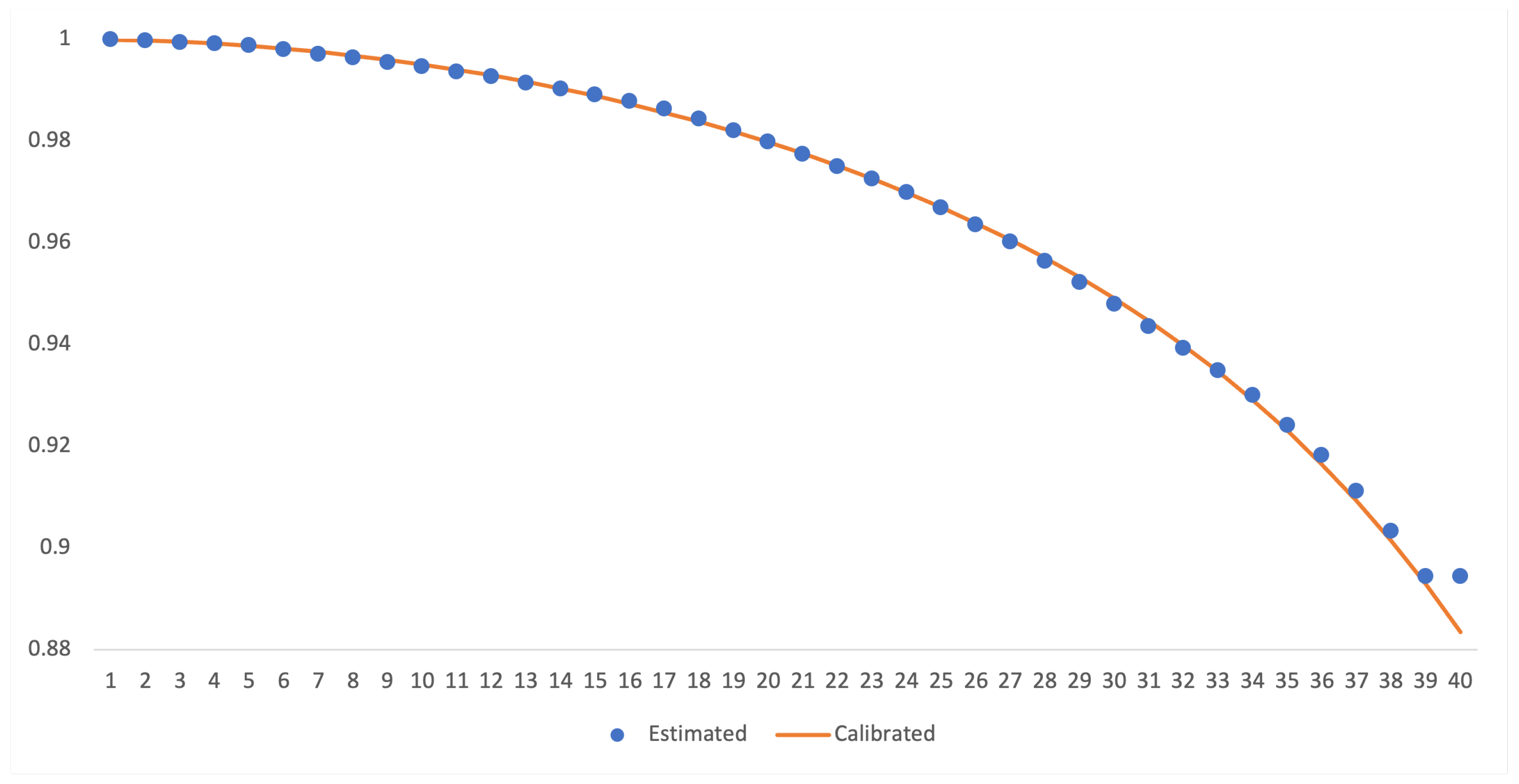
The coefficient a reflects a quadratic term, suggesting a decreasing survival probability as time progresses. b is effectively negligible, while c and d end up governing the baseline and exponential growth. Figure 3 represents the calibration versus the estimated values, showing a very good fit.

4.1. Hazard Functions

We can use the calibrated survival function above to derive other key variables.
From Equation (2), we can obtain the hazard values from our Gompertz–Makeham survival function:
h G M ( t ) = t log [ S G M ( t ) ] , h G M ( t ) = 0.000086088 t + 6.820428518109184 × 10 23 + 2.999564228 × 10 5 e 0.138564 t ,
which represent the calibrated instantaneous rate of occurrence of default on a loan at each age or time point. In the context of a loan portfolio, the hazard value indicates the probability that a borrower defaults on their loan within a specific age or time interval ( [ t , t + d t [ ) , given that they have survived up to that point ( t ) .
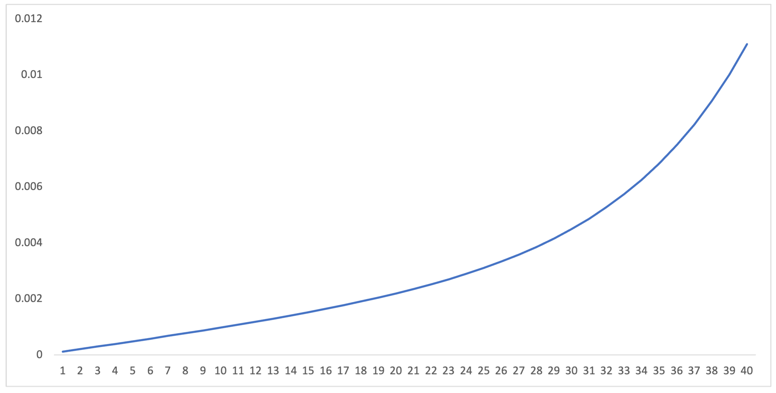
Figure 4 represents the hazard function corresponding to a Gompertz–Makeham fitting to the survival function. As the age or time interval increases, the hazard value also rises. The increasing hazard values imply that the likelihood of experiencing default tends to grow as time progresses.

4.2. Default Probabilities

The probability density of default defined in (6). f ( t ) is related to the hazard function and the survival function by the following:
f G M ( t ) = h G M ( t ) S G M ( t ) .
Simplifying from (2), we obtain f G M ( t ) = S G M ( t ) , where ′ denotes the derivative.
Finally, given the previous calibration, we get
f G M ( t ) = 1.00021664346381 0.000086088 t + 3.001573368 × 10 5 · e 0.138564 t + 6.820428518109184 × 10 23 × × exp 0.000043044 t 2 6.820428518109184 × 10 23 t 0.00021662 · e 0.138564 t .
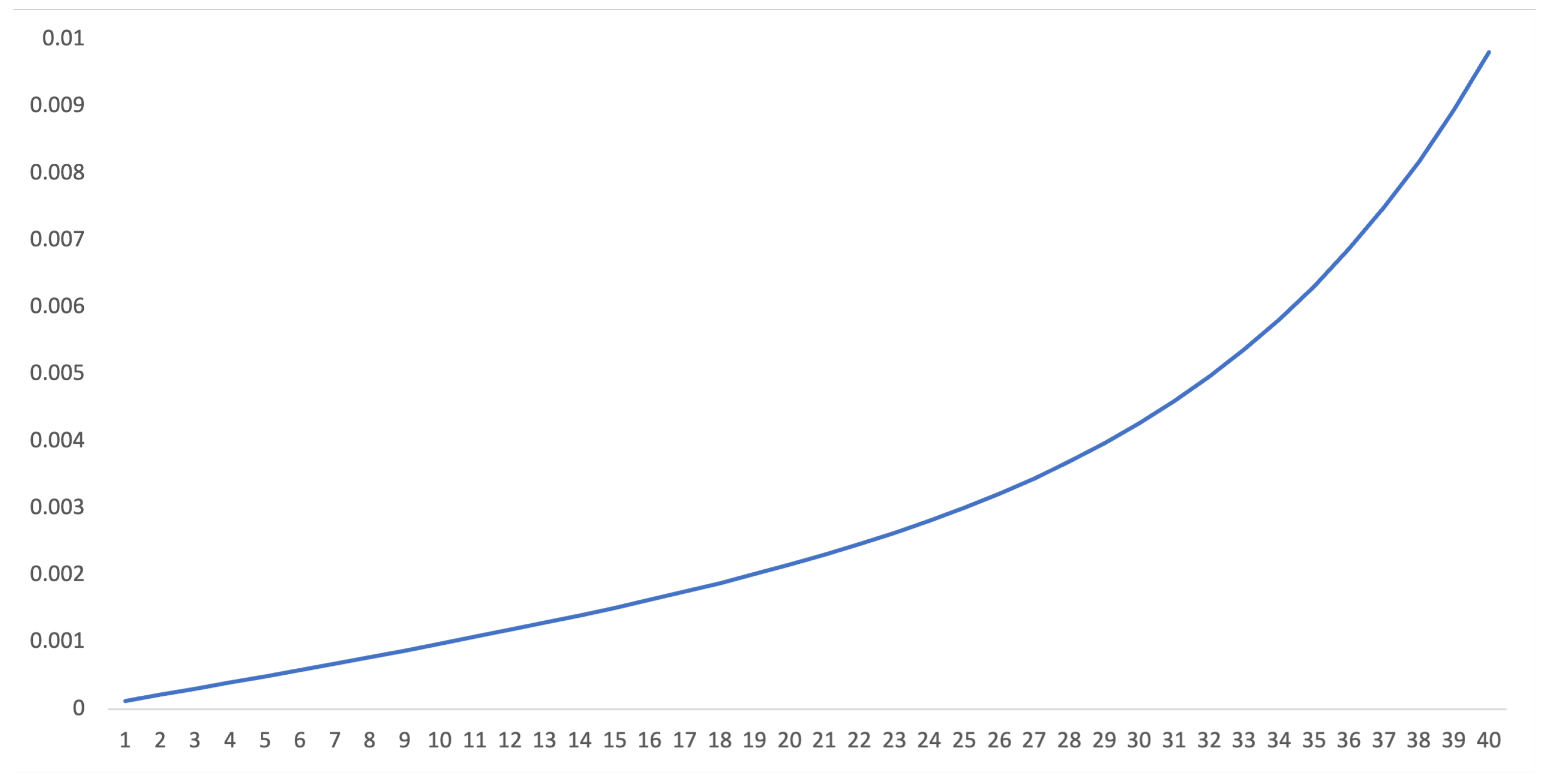
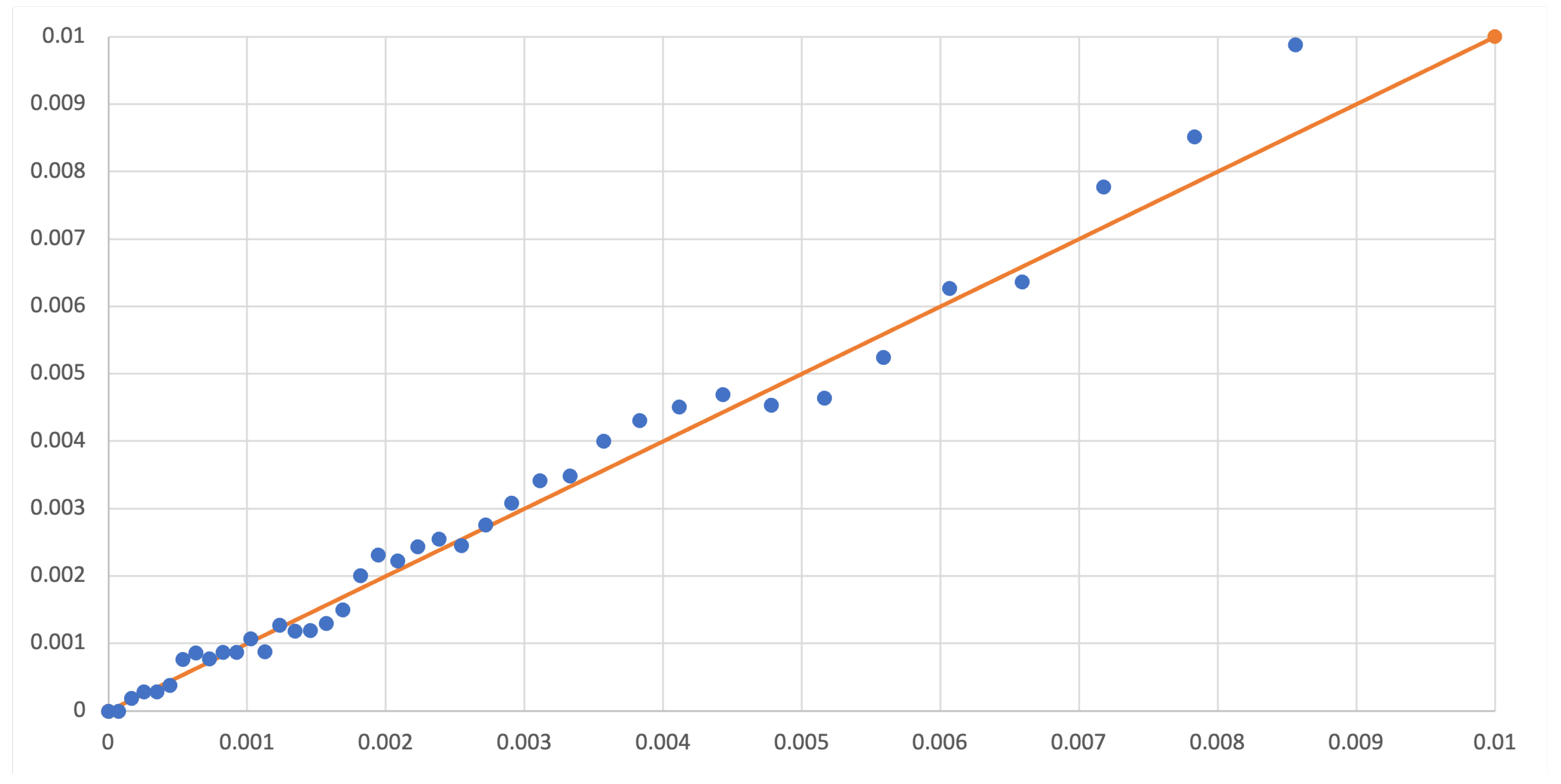
Figure 5 shows the calibrated density of defaults. Figure 6 compares probabilities of default from the calibrated model against the estimated probabilities of default from Table 1. It shows that although the fit is not perfect, its closeness to the 45-degree line attest the quality of our calibration, along with the Brier Score for the calibration curve of 3.64241333364887 × 10⁻⁶, indicating very low mean squared differences (Brier 1950; Steyerberg et al. 2010).
Given the density of defaults, the actual number of defaults can be obtained, provided that we also establish a framework for the number of loans at risk at each moment in time, N ( t ) . Accurately defining defaults at risk requires accounting for right censoring and properly integrating attrition effects. That is, calibrating the estimated number of loans at risk, n j from Table 1, is crucial to model the number of default occurrences at each time interval.
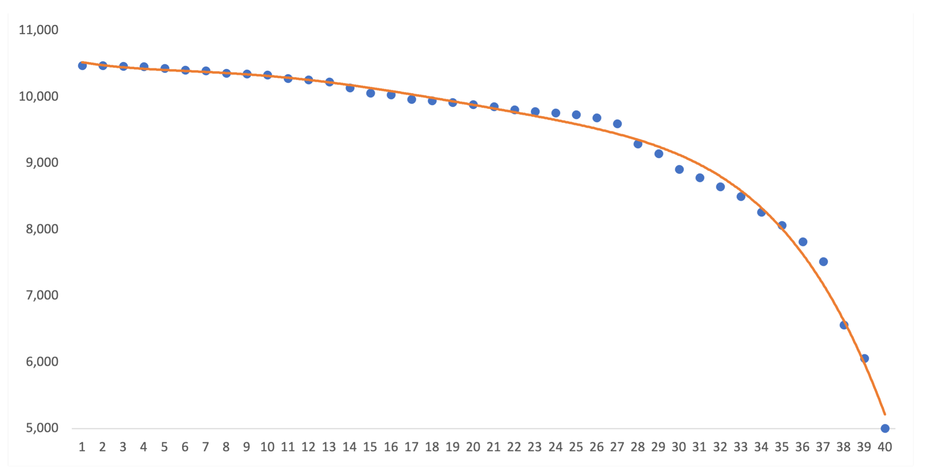
From Figure 7 we see the number of loans at risk in our portfolio does not need more than a polynomial fit. So we use
N p o l ( t ) = 0.0124 × t 4 + 0.07716 3 16.7 t 2 + 102 t + 10600 .
To obtain the number of defaults we use Equation (7) to get
d G M ( t ) = N p o l ( t ) f G M ( t ) .
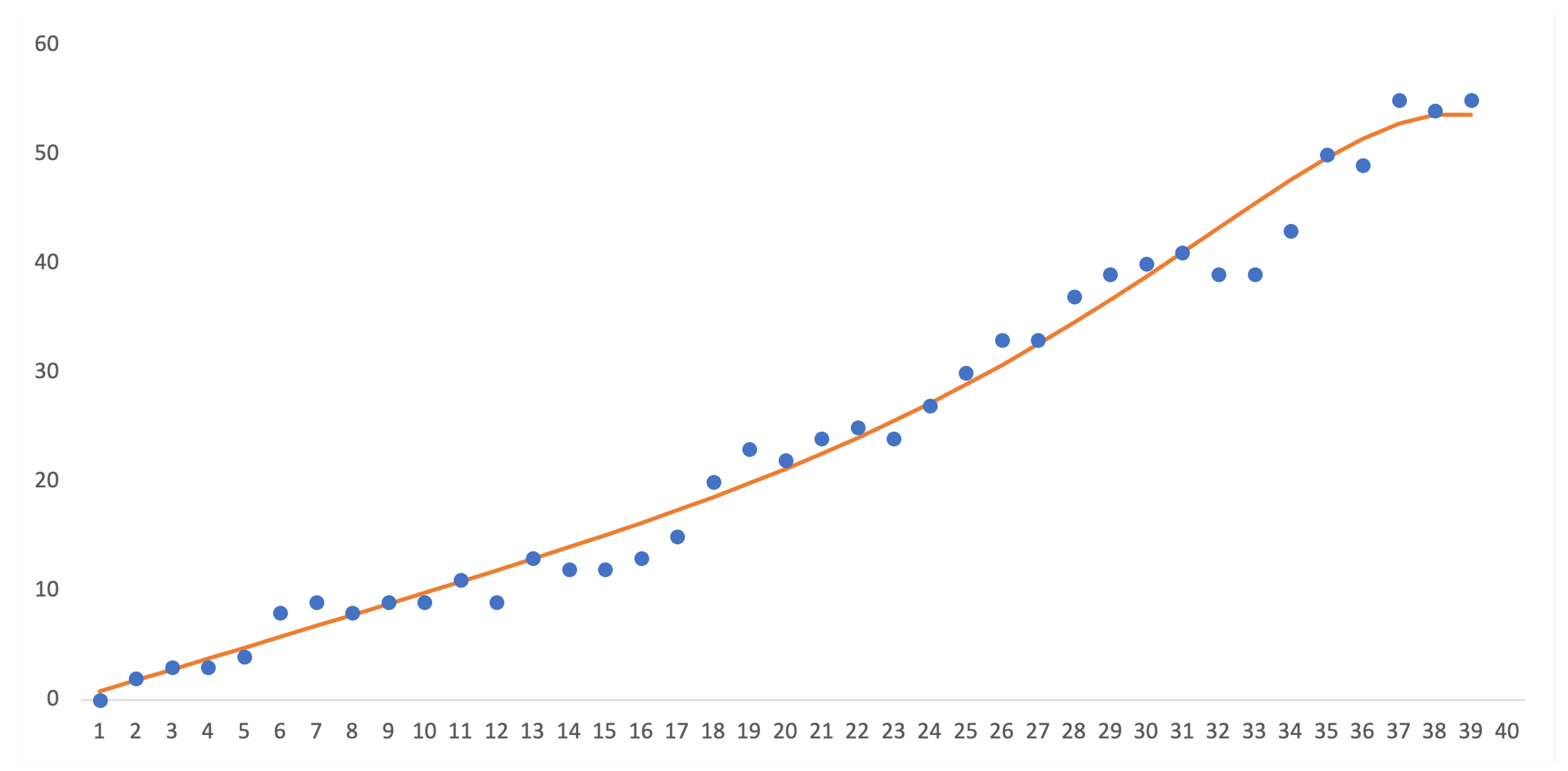
Figure 8 displays the estimated number of defaults, q j , from Table 1, alongside the calibrated function d G M ( t ) .
As we proceed with the analysis, it is important to exercise caution when interpreting results near maturity, given this potential underestimation.
In practical applications, on the one at hand, we may need to be able to simulate the number of defaults per time interval I j = [ t j 1 , t j ] . By now we already have all ingredients and we are only missing a distribution for the number of defaults, which we can take as a non-homogeneous Poisson process, where the default intensity varies over time:
P ( d j = k ) = Λ ( t j 1 , t j ) k e Λ ( t j 1 , t j ) k ! , k = 0 , , +
where
Λ ( t j 1 , t j ) = t j 1 t j h ( t ) S ( t ) N ( t ) d t .
The Poisson distribution is a natural choice for modeling defaults within a survival analysis framework, particularly when defaults are viewed as rare, discrete events occurring over time. In this context, the number of defaults in a given interval can be modeled as a Poisson process, with the mean linked directly to the default intensity (hazard rate) and the number of loans at risk.
This approach is especially suitable when default intensities are known or can be estimated from historical data, allowing the Poisson mean to reflect time-varying risk.
Assuming the survival function, hazard rates and the number of loans at risk are approximately constant in each interval I j = [ t j 1 , t j ] , we get
Λ ( t j 1 , j ) h ( t j 1 ) S ( t j 1 ) N ( t j 1 ) ( t j t j 1 ) .
In our case we use S G M , h G M , and N p o l , from Equations (11), (12), and (13), respectively.
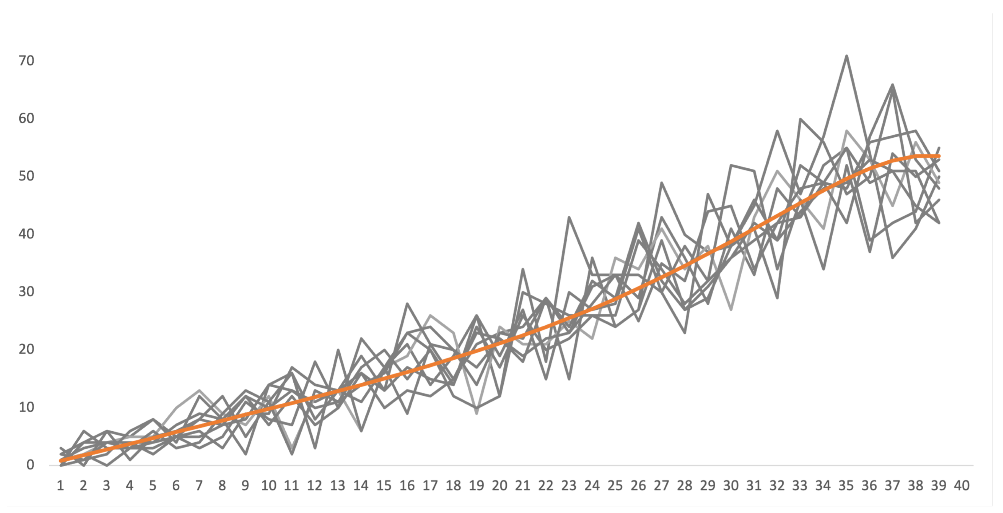
Figure 9 displays 10 simulated paths of the number of defaults, generated using our calibrated functions. For each time interval I j = [ t j 1 , t j ] , the cumulative intensity Λ j is computed as in Equation (16), and default counts are drawn using the inverse of the Poisson probability function defined in Equation (15).
It is interesting to note that the simulations not only capture the tendency for the number of defaults to increase as maturity approaches, but also reveal a rise in the volatility of potential defaults. This increase in variability stems from the uncertainty of results—larger default numbers naturally lead to greater fluctuations. These findings further confirm that the use of the Poisson distribution is appropriate.

4.3. Loss Given Default

Although our empirical data lacks direct information on losses given a default, a comprehensive credit risk assessment requires this crucial insight.
For simplicity, we assume an homogeneous portfolio, where all 10,479 loans share the same notional value of 25,000 monetary units (m.u.). The portfolios is, thus, worth 261,975,000 m.u. initially. Furthermore, we estimate the average loss given default to be 40% of the notional, amounting to 10,000 m.u. per loan.
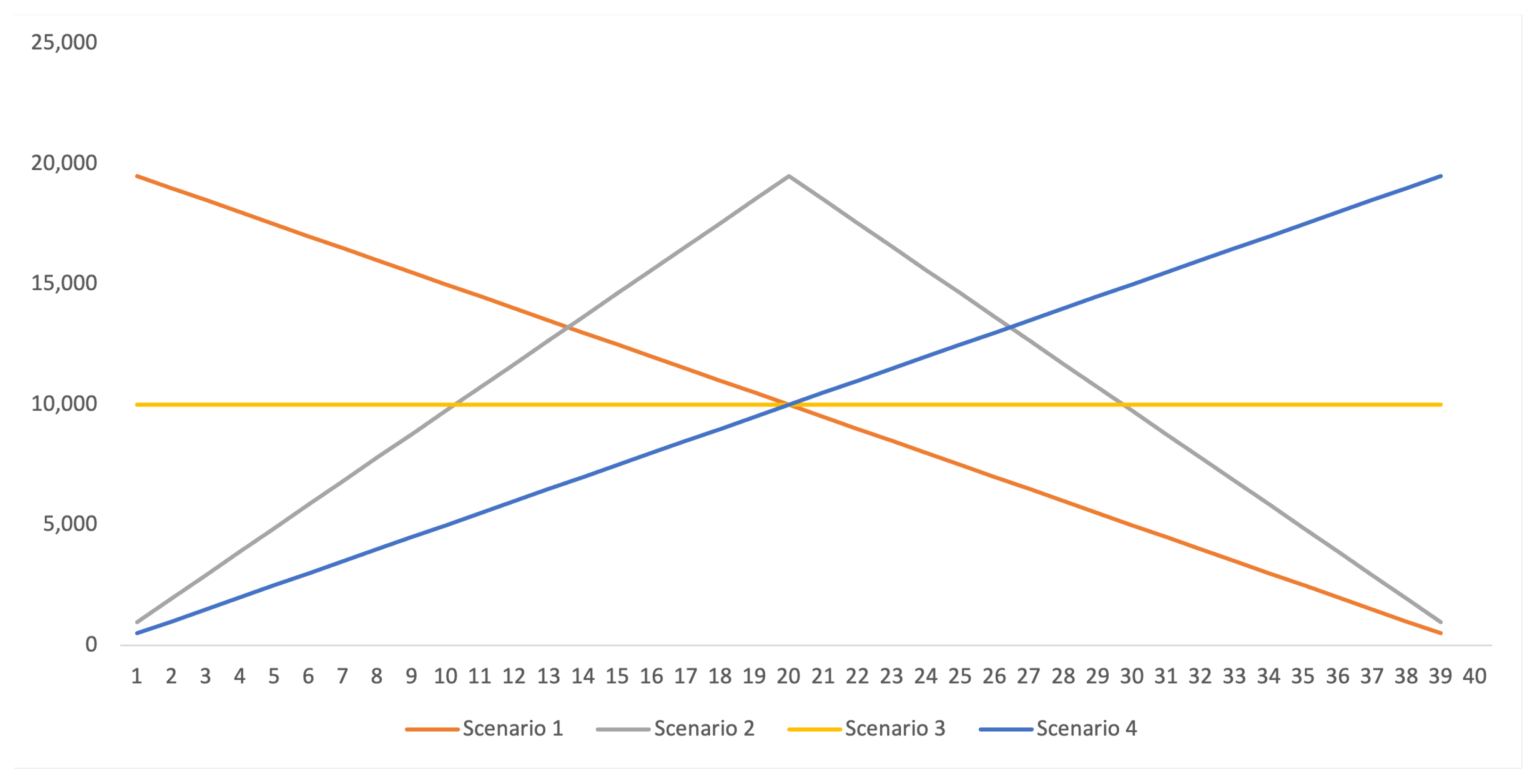
We assume a 40% loss on average, but different scenarios in terms of the functional form of our loss function, l ( t ) , over time:
  • Decreasing: l ( t ) = ( M t ) × 500 .
  • Increasing then Decreasing: l ( t ) = t × 975 for t 20 , l ( t ) = ( M t ) × 975 for t > 20 .
  • Constant: l ( t ) = 10 , 000 .
  • Increasing: l ( t ) = t × 500 .
Scenario 1 recognizes that as maturity approaches, previous payments remain intact, reducing potential losses over time. Naturally, losses diminish as the loan nears completion—in the extreme case, when only one final payment is due, the loss is minimal. The multiplication by 500 ensures that the average loss remains at 10,000 m.u., maintaining comparability across different loss functions.
Scenario 2 considers a more complex pattern, where losses initially increase before declining as the credit matures.
Scenario 3 assumes a naïve approach, where a default at any point in time consistently results in a fixed loss of 10,000 m.u., regardless of when it occurs.
Finally, Scenario 4 explores an opposite trend, modeling steadily increasing losses over time.
While scenarios 2 and 4 may lack direct economic interpretability, their inclusion allows us to examine diverse possibilities in the absence of a confirmed empirical loss given default process. Figure 10 shows the four scenarios under consideration.
In reality, loss given default (LGD) is likely to follow a non-linear pattern, and we only observe discrete data points that should be calibrated using a non-linear function. The calibrated function can then serve as the foundation for computing the loss process and key risk measures. In this analysis, however, we apply the previously defined scenarios’ functions.
It is important to note that the above approach provides LGD as a function of time but does not yield the aggregated loss process. The latter depends on the actual number of defaults at each point in time from the previous section.
In the next section, we bring all these elements together to construct a comprehensive view of the loss dynamics.

4.4. Loss Process

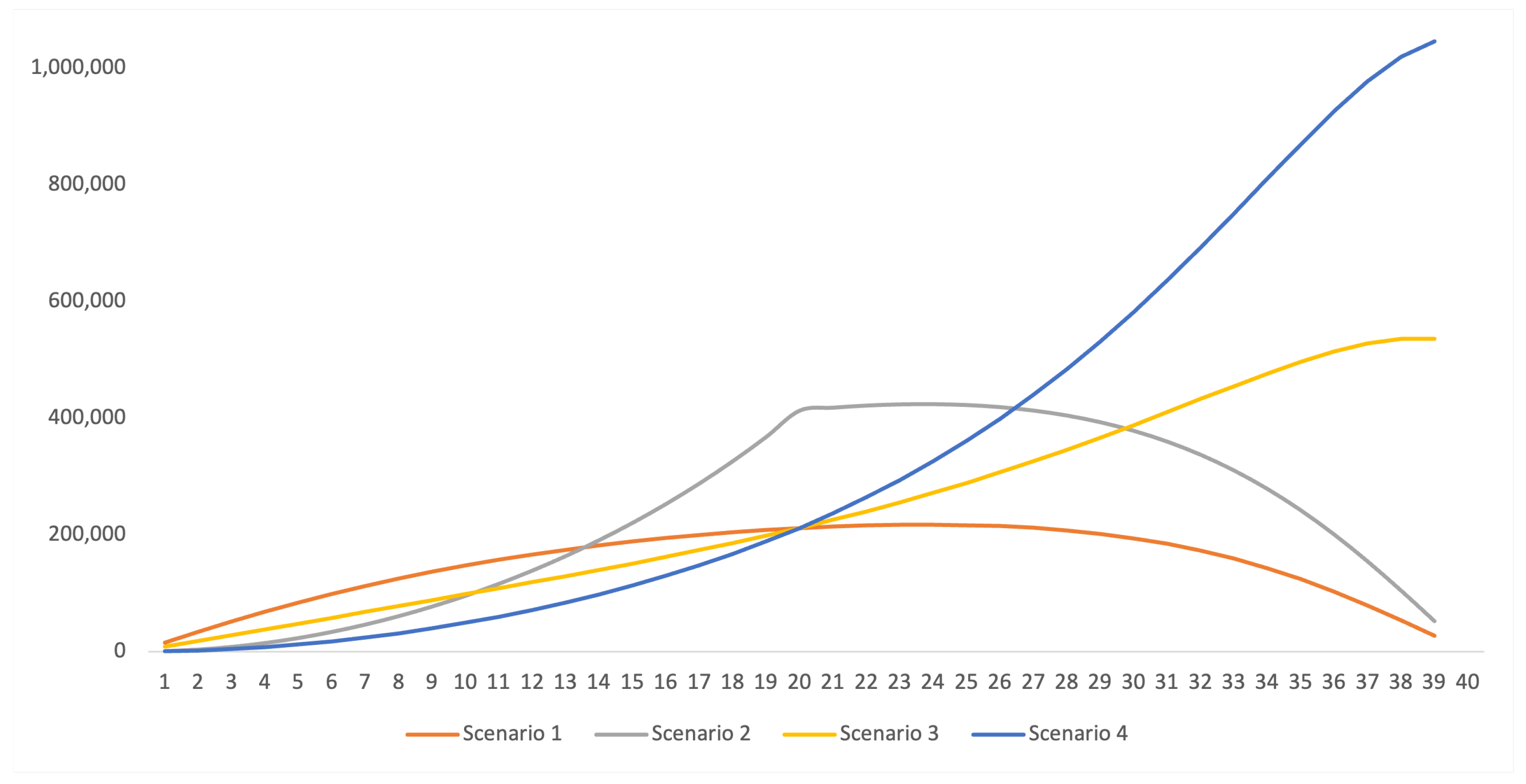
To determine the evolution of the loss process, L ( t ) , over time, we need two ingredients: (i) the number of defaults over time, d G M ( t ) (from Equation (6)), and (ii) the loss given default over time, l ( t ) (as defined in the previous section),
L ( t ) = d G M ( t ) × l ( t ) .
Figure 11 shows the loss process, L ( t ) , associated with the four scenarios for loss given default, and assuming the calibrated function for d G M as in Figure 8.
Notice that the change in the pattern of LGD leads to very different loss processes. When LGD is considered constant (Scenario 3), of course the loss function inherits the shape of the number of defaults d G M ( t ) . When LGD decreases with the age of the loan (Scenario 1), we see the loss process starts by increasing, but from approximately age 20 onwards, it actually decreases, despite the fact that the number of defaults increase over time. Scenarios 2 and 4 are less realistic, but the point here is to show the evolution of losses over time and to show they are determined by both default probability and LGD, and one should not neglect modeling LGD for proper modeling of credit risk.

4.5. Computing Risk Measures

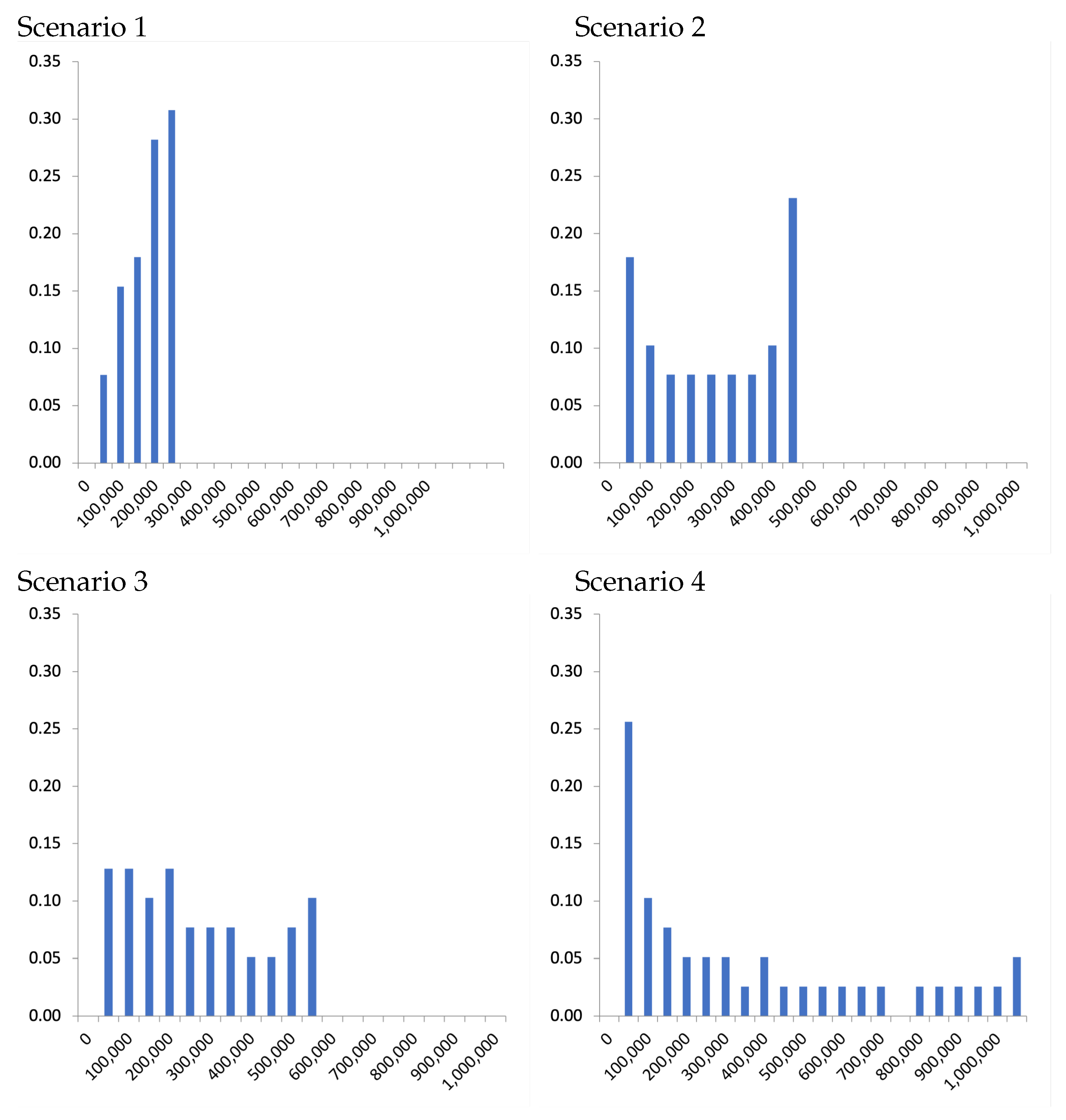
The classical approach to risk measurement involves estimating standard credit risk metrics based on the distribution of the four loss processes under consideration. Figure 12 displays the histograms of the loss processes associated with these four scenarios (from Figure 11). Table 2 presents the corresponding values for Value at Risk (VaR) and Expected Shortfall (ES) for each scenario.
Both VaR and ES vary considerably depending on the assumed LGD scenario. Notably, the most realistic case—Scenario 1—yields values less than half of those obtained under a constant LGD assumption (Scenario 3), providing a strong incentive to model LGD accurately for reliable credit risk assessment.
Both the histograms and the risk measures presented thus far, however, do not account for the time structure of the loans’ age—that is, they reflect losses aggregated on an annual basis without considering the specific timing within the loans’ lifetimes. As a result, these measures are associated with annual losses, independently of ages of the loans.
From the discussions throughout the paper, it is evident that the risk profile of a loan aged 1-year is not the same as that of a loan with, for example, 20-years. The primary purpose of employing survival analysis is in fact to explicitly incorporate the timing and duration aspects into the risk assessment. Fortunately, we have all the necessary tools to compute risk measures that are adapted to the varying ages of the different loans.
To generate Figure 12, we used the calibrated function d G M ( t ) shown in Figure 8. Now, we perform simulations similar to those illustrated in Figure 9, but instead of 10 paths, we consider 10,000 paths. Each simulation path multiplies the four possible LGD profiles depicted in Figure 11.
Thus, for each scenario in terms of LGD, we obtain 10,000 possible loss outcomes at each loan age. This approach enables us to obtain the distribution of losses per age of loan and compute the associated VaR and ES, providing a much deeper understanding of the risk profile of our loan portfolio.
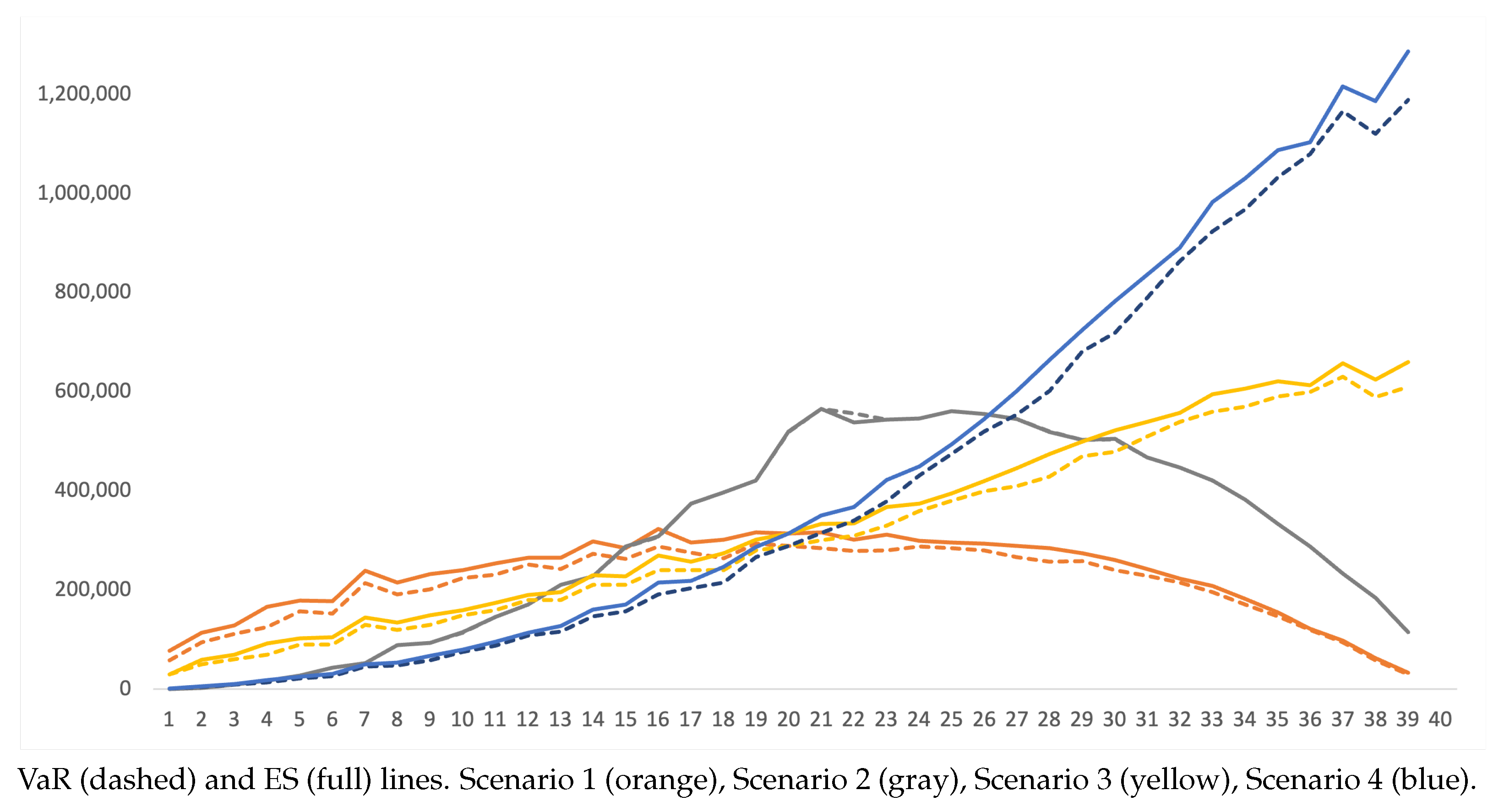
Having the densities, we can obtain VaR and ES which are age-specific statistics that differ according to the loans’ age. Table 3 presents the numerical results for VaR and ES, while Figure 13 provides a visual illustration of the 95% VaR and ES across different scenarios. The figure clearly shows how both risk measures vary with the age of the loans, reflecting the influence of the underlying LGD profiles depicted in Figure 11. It also highlights how this age-sensitive approach delivers a far more rigorous and informative view than traditional, static risk metrics.
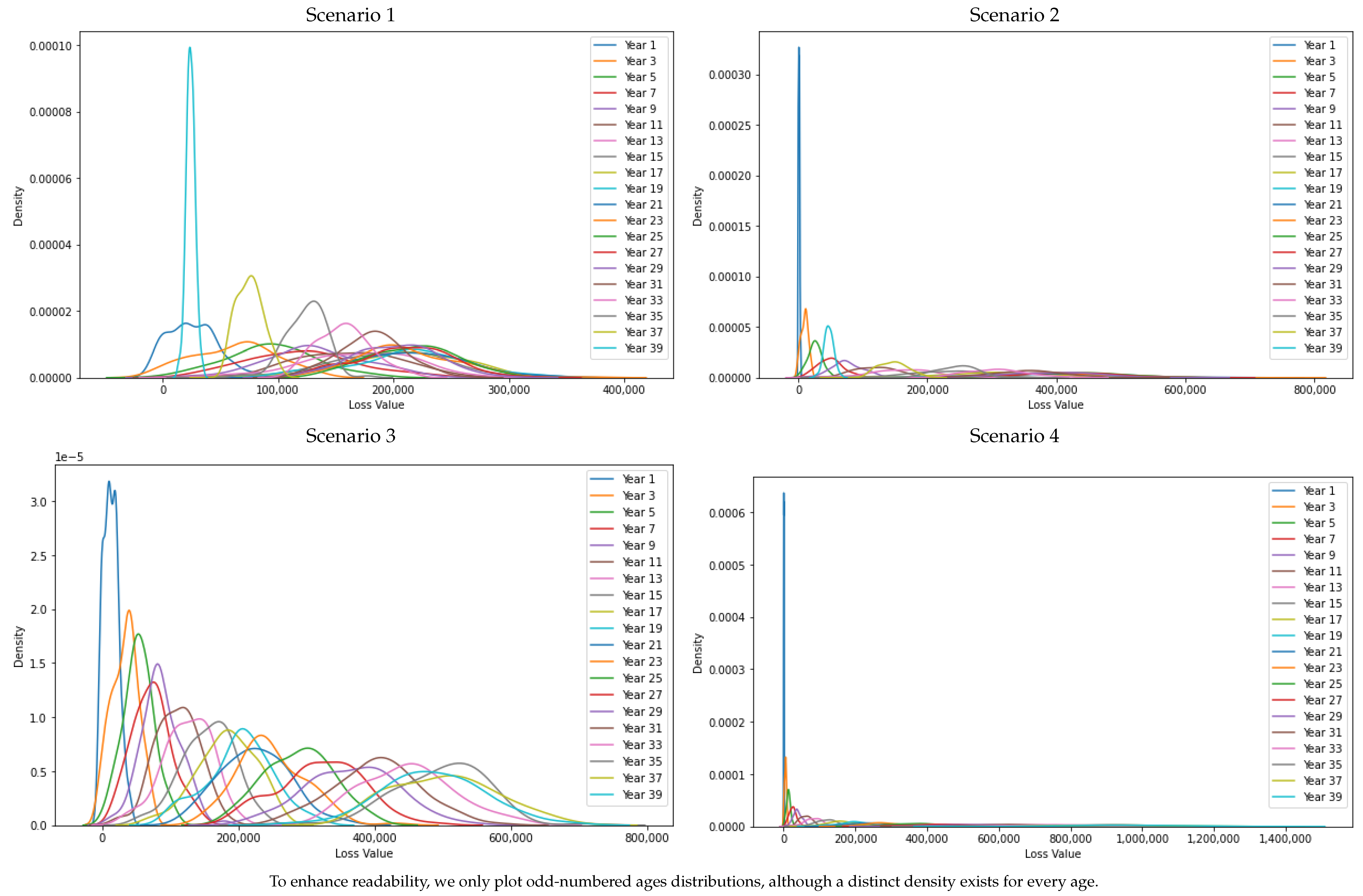
Figure 14 presents the density functions of losses obtained from the simulations across different scenarios and loan ages. Because the scales of the graphs differ, direct comparisons are not straightforward. Nonetheless, one clear pattern emerges: across all scenarios, the loss densities change with loan age, highlighting the dynamic nature of the risk profile over time. Note that losses under Scenario 1 exhibit the lowest values, whereas Scenario 4 shows the highest. This contrast directly reflects the structure of the underlying loss processes shown in Figure 11.
By explicitly accounting for loan age, this methodology reveals how credit risk evolves over time—something standard measures often obscure. Even when using familiar statistics like VaR and ES, the results differ meaningfully across loan age cohorts, underscoring the value of a dynamic perspective for risk assessment and portfolio management.

5. Managerial and Policy Implications

The survival analysis framework developed in this study carries significant practical implications for financial institutions and regulators, particularly in emerging markets where data limitations and dynamic risk profiles present unique challenges. For bank management, this approach enables dynamic risk monitoring through age-dependent metrics like VaR and ES, which evolve over a loan’s life cycle. For instance, in the case of the Angolan banks we analyzed, our results show that the 95% VaR for Scenario 1 increases from 58,500 monetary units in Year 1 to 209,095 close to maturity, underscoring the need for progressive capital allocation and early interventions for aging portfolios.
For pricing and provisioning decisions, the Gompertz–Makeham hazard function reveals how default risk escalates over time. This insight allows banks to adjust credit spreads for longer-term loans and front-load loss provisions. The framework’s adaptability to portfolio-specific data also supports targeted risk mitigation, such as restructuring high-risk cohorts before hazards peak.
From a regulatory perspective, this methodology directly supports Basel IRB compliance by providing time-to-default probabilities and age-sensitive LGD estimates. Central banks in emerging markets could adopt it as a standardized approach for institutions lacking ML capabilities, as advocated by recent studies on interpretable models. The model’s extendibility to macroeconomic variables further enables regulators to stress-test portfolios under commodity price shocks or GDP contractions, informing countercyclical capital buffer policies.
However, broader implementation requires the addressing of two systemic gaps. First, the lack of LGD data in emerging markets remains a critical limitation, as our scenarios demonstrate VaR estimates vary by 110% across LGD assumptions. Second, the Poisson distribution may underestimate tail risk in volatile economies, suggesting a need for hybrid approaches. Policymakers can mitigate these gaps by incentivizing shared credit registries and standardizing loan age data collection, building on initiatives like the EU’s AnaCredit system.

6. Conclusions

This paper demonstrates how survival analysis offers a robust, interpretable alternative to traditional credit risk models, particularly for emerging markets operating under the Basel IRB framework.
The proposed approach is grounded in survival analysis and centers on the calibration of key functions, such as the survival function and the number of loans at risk over time. It assumes a Poisson distribution for the number of defaults. We apply this methodology to a real dataset from 10 Angolan banks, comprising 10,479 loans. Based on this information, we fully characterize the probability of default—one of the core components of the IRB framework. Additionally, we simulate default paths conditional on the age of each loan.
Unfortunately, the dataset does not include information on loss given default (LGD), another essential element of the IRB framework, nor does it allow for holdout validation. To address the loss limitation, we explore several LGD scenarios and demonstrate that in shaping the final loss distribution and standard risk metrics—such as Value at Risk (VaR) and Expected Shortfall (ES)—the LGD profile is at least as influential as the default profile. While LGD data was unavailable in our case, such information is typically accessible to banks through historical experience, making its calibration feasible in practice.
Building on the strengths of the survival-based approach, we also propose calculating risk measures conditional on loan age. These age-dependent metrics offer significantly more insight than traditional aggregated risk statistics. Our results reveal that loss densities vary meaningfully with loan age—an aspect that should not be overlooked, especially since such conditional information can be easily derived through simple simulations. To the best of our knowledge, this is the first study to compute VaR and ES as functions of loan age in the context of credit risk evaluation.
Throughout our application, we calibrated functional forms for key variables—such as the survival function and the number of loans at risk—to reflect the structure of our dataset. These calibrations achieved a strong empirical fit, though other datasets may require alternative specifications to accommodate different portfolio characteristics or risk dynamics. For modeling defaults, we relied on the Poisson distribution, a widely used and intuitive choice for count data. However, alternative distributions—such as the Negative Binomial or Binomial—may be more suitable in contexts where default counts exhibit greater variability or are constrained by the number of exposures.
Future research could focus on obtaining and incorporating empirical data on LGD, which would improve the calibration of loss distributions and enhance the accuracy of associated risk measures like VaR and ES. Moreover, integrating macroeconomic or borrower-specific covariates into the survival and LGD models could capture additional risk drivers and improve predictive power. Finally, linking the model’s outputs to capital planning and stress testing processes would increase its practical relevance for both regulatory compliance and strategic risk management.

Author Contributions

Conceptualization, F.L.D., M.L.E. and R.M.G.; methodology, F.L.D., M.L.E. and R.M.G.; software, F.L.D. and R.M.G.; validation, M.L.E. and R.M.G.; formal analysis, F.L.D., M.L.E. and R.M.G.; investigation, F.L.D., M.L.E. and R.M.G.; resources, F.L.D., M.L.E. and R.M.G.; data curation, F.L.D.; writing—original draft preparation, R.M.G.; writing—review and editing, R.M.G.; visualization, F.L.D. and R.M.G.; supervision, M.L.E. and R.M.G.; project administration, R.M.G.; funding acquisition, M.L.E. and R.M.G. All authors have read and agreed to the published version of the manuscript.

Funding

MLE work was partially supported by national resources through the FCT—Fundação para a Ciência e a Tecnologia, I.P., under the scope of the project UIDB/00297/2020 and project UIDP/00297/2020. RMG work was partially supported by FCT, I.P., the Portuguese national funding agency for science, research and technology, under the Project UID06522.

Data Availability Statement

The empirical data used in this study was collected from 10 Angolan banks and is fully disclosed on Table 1. All remaining data is simulated using the methods described.

Conflicts of Interest

The views expressed in this paper are those of the authors and do not necessarily reflect those of the Banco Nacional de Angola; this study was conducted solely for academic purposes. The authors also declare no other conflicts of interest.

References

  1. Abdalla, Hemn Barzan, Yulia Kumar, Jose Marchena, Stephany Guzman, Ardalan Awlla, Mehdi Gheisari, and Maryam Cheraghy. 2025. The future of artificial intelligence in the face of data scarcity. Computers, Materials & Continua 84: 1–27. [Google Scholar] [CrossRef]
  2. Baesens, Bart, Tony Van Gestel, Maria Stepanova, Dirk Van den Poel, and Jan Vanthienen. 2005. Neural network survival analysis for personal loan data. Journal of the Operational Research Society 56: 1089–98. [Google Scholar] [CrossRef]
  3. Banasik, John, Jonathan N. Crook, and Lyn C. Thomas. 1999. Not if but when will borrowers default. Journal of the Operational Research Society 50: 1185–90. [Google Scholar] [CrossRef]
  4. BCBS. 2011. Basel III: A Global Regulatory Framework for More Resilient Banks and Banking Systems Revised Version June 2011. Basel: Basel Committee on Banking Supervision. [Google Scholar]
  5. BIS. 2006. Basel II: International Convergence of Capital Measurement and Capital Standards: A Revised Framework-Comprehensive Version. Bank for International Settlements. Available online: https://www.bis.org/publ/bcbs128.htm (accessed on 1 August 2025).
  6. Bo, Wang. 2024. The impact of macroeconomic factors on credit risk management in developing country banks: An analysis based on basel III. Financial Engineering and Risk Management 7: 97–105. [Google Scholar] [CrossRef]
  7. Borisov, Vadim, Tobias Leemann, Kathrin Seßler, Johannes Haug, Martin Pawelczyk, and Gjergji Kasneci. 2022. Deep neural networks and tabular data: A survey. IEEE Transactions on Neural Networks and Learning Systems 35: 7499–519. [Google Scholar] [CrossRef]
  8. Brier, Glenn W. 1950. Verification of forecasts expressed in terms of probability. Monthly Weather Review 78: 1–3. [Google Scholar] [CrossRef]
  9. Charpignon, Marie-Laure, Enguerrand Horel, and Flora Tixier. 2014. Prediction of Consumer Credit Risk. Stanford: Standford University. [Google Scholar]
  10. Crosbie, Peter, and Jeff Bohn. 2003. Modeling Default Risk: Modeling Methodology. San Francisco: KMV Corporation. [Google Scholar]
  11. Derbali, Abdelkader. 2018. How the Default Probability Is Defined by the Creditrisk+ Model? Available online: https://hal.science/hal-01696011v1 (accessed on 1 August 2025).
  12. Dickson, David C. M., Mary Hardy, Mary R. Hardy, and Howard R. Waters. 2013. Actuarial Mathematics for Life Contingent Risks. Cambridge: Cambridge University Press. [Google Scholar]
  13. Djeundje, Viani Biatat, and Jonathan Crook. 2019. Dynamic survival models with varying coefficients for credit risks. European Journal of Operational Research 275: 319–33. [Google Scholar] [CrossRef]
  14. Erkkilä, Rami. 2025. Interpretable machine learning for credit risk predictions. Economic Review 105: 315–20. [Google Scholar]
  15. Fejza, Doris, Dritan Nace, and Orjada Kulla. 2022. The credit risk problem—A developing country case study. Risks 10: 146. [Google Scholar] [CrossRef]
  16. Gompertz, Benjamin. 1825. Xxiv. on the nature of the function expressive of the law of human mortality, and on a new mode of determining the value of life contingencies. in a letter to francis baily, esq. frs &c. Philosophical Transactions of the Royal Society of London 115: 513–83. [Google Scholar]
  17. Hassan, M. Kabir, Jennifer Brodmann, Blake Rayfield, and Makeen Huda. 2018. Modeling credit risk in credit unions using survival analysis. International Journal of Bank Marketing 36: 482–95. [Google Scholar] [CrossRef]
  18. Hernes, Marcin, Jędrzej Adaszyński, and Piotr Tutak. 2023. Credit risk modeling using interpreted xgboost. European Management Studies 21: 46–70. [Google Scholar] [CrossRef]
  19. Huang, Haonan, Jing Li, Chundan Zheng, Sikang Chen, Xuanyin Wang, and Xingyan Chen. 2025. Advanced default risk prediction in small and medum-sized enterprises using large language models. Applied Sciences 15: 2733. [Google Scholar] [CrossRef]
  20. Hurlin, Christophe, and Christophe Pérignon. 2023. Machine Learning and Irb Capital Requirements: Advantages, Risks, and Recommendations. Jouy-en-Josas: HEC Paris. Available online: https://ideas.repec.org/p/ebg/heccah/1480.html (accessed on 1 August 2025).
  21. Kakadiya, Rushikesh, Tarannum Khan, Anjali Diwan, and Rajesh Mahadeva. 2024. Transformer models for predicting bank loan defaults a next-generation risk management. Paper presented at 2024 IEEE 6th International Conference on Cybernetics, Cognition and Machine Learning Applications (ICCCMLA), Hamburg, Germany, October 19–20; pp. 26–31. [Google Scholar]
  22. Kaplan, Edward L., and Paul Meier. 1958. Nonparametric estimation from incomplete observations. Journal of the American Statistical Association 53: 457–81. [Google Scholar] [CrossRef]
  23. Kleinbaum, David G., and Mitchel Klein. 2012a. Survival Analysis: A Self-Learning Text. Berlin and Heidelberg: Springer. [Google Scholar]
  24. Kleinbaum, David G., and Mitchel Klein. 2012b. Survival Analysis. Statistics for Biology and Health, 3rd ed. New York: Springer. [Google Scholar]
  25. Kragh Jørgensen, Rasmus Rask, Faartoft Jonas Jensen, Tarec El-Galaly, Martin Bøgsted, Rasmus Froberg Brøndum, Mikkel Runason Simonsen, and Lasse Hjort Jakobsen. 2025. Development of time to event prediction models using federated learning. BMC Medical Research Methodology 25: 143. [Google Scholar] [CrossRef]
  26. Leo, Martin, Suneel Sharma, and Koilakuntla Maddulety. 2019. Machine learning in banking risk management: A literature review. Risks 7: 29. [Google Scholar] [CrossRef]
  27. Mahbobi, Mohammad, Salman Kimiagari, and Marriappan Vasudevan. 2023. Credit risk classification: An integrated predictive accuracy algorithm using artificial and deep neural networks. Annals of Operations Research 330: 609–37. [Google Scholar] [CrossRef]
  28. Makeham, William Matthew. 1860. On the law of mortality and the construction of annuity tables. Journal of the Institute of Actuaries 8: 301–10. [Google Scholar] [CrossRef]
  29. McDonald, Ross A., Ania Matuszyk, and Lyn C. Thomas. 2010. Application of survival analysis to cash flow modelling for mortgage products. OR Insight 23: 1–14. [Google Scholar] [CrossRef]
  30. Micocci, Marco. 2000. MARC: An actuarial model for credit risk. Paper presented at ASTIN Colloquium 2000, Porto Cervo, Italy, September 17–20, vol. 31. [Google Scholar]
  31. Poudel, Ravi Prakash Sharma. 2013. Macroeconomic determinants of credit risk in nepalese banking industry. Paper presented at 21st International Business Research Conference, Toronto, ON, Canada, June 10–11; pp. 10–11. [Google Scholar]
  32. Rocha, Cristina, and Ana Luísa Papoila. 2009. Análise de Sobrevivência. Portugal: Sociedade Portuguesa de Estatística. [Google Scholar]
  33. Sharma, Alok Kumar, Li-Hua Li, and Ramli Ahmad. 2022. Default risk prediction using random forest and xgboosting classifier. In 2021 International Conference on Security and Information Technologies with AI, Internet Computing and Big-data Applications. Berlin and Heidelberg: Springer, pp. 91–101. [Google Scholar]
  34. Siphuma, Elekanyani, and Terence van Zyl. 2025. Enhancing credit risk assessment through transformer-based machine learning models. In Artificial Intelligence Research. SACAIR 2024. Communications in Computer and Information Science. Edited by Aurona Gerber, Jacques Maritz and Anban W. Pillay. Berlin and Heidelberg: Springer, vol. 2326. [Google Scholar]
  35. Smith, Peter J. 2017. Analysis of Failure and Survival Data. Boca Raton: CRC Press. [Google Scholar]
  36. Stepanova, Maria, and Lyn Thomas. 2002. Survival analysis methods for personal loan data. Operations Research 50: 277–89. [Google Scholar] [CrossRef]
  37. Steyerberg, Ewout W., Andrew J. Vickers, Nancy R. Cook, Thomas Gerds, Mithat Gonen, Nancy Obuchowski, Michael J. Pencina, and Michael W. Kattan. 2010. Assessing the performance of prediction models: A framework for traditional and novel measures. Epidemiology 21: 128–38. [Google Scholar] [CrossRef] [PubMed]
  38. Suisse Credit. 1997. Creditrisk+, A Credit Risk Management Framework. London: Credit Suisse Financial Products. [Google Scholar]
  39. Zhang, Dongfang, Basu Bhandari, and Dennis Black. 2021. Covariate selection for mortgage default analysis using survival models. Journal of Mathematical Finance 11: 218–33. [Google Scholar] [CrossRef]
  40. Zokirjonov, Mukhammadsodik. 2018. Methodology of creditmetrics for credit risk assessment. International Finance and Accounting 2018: 135. [Google Scholar]
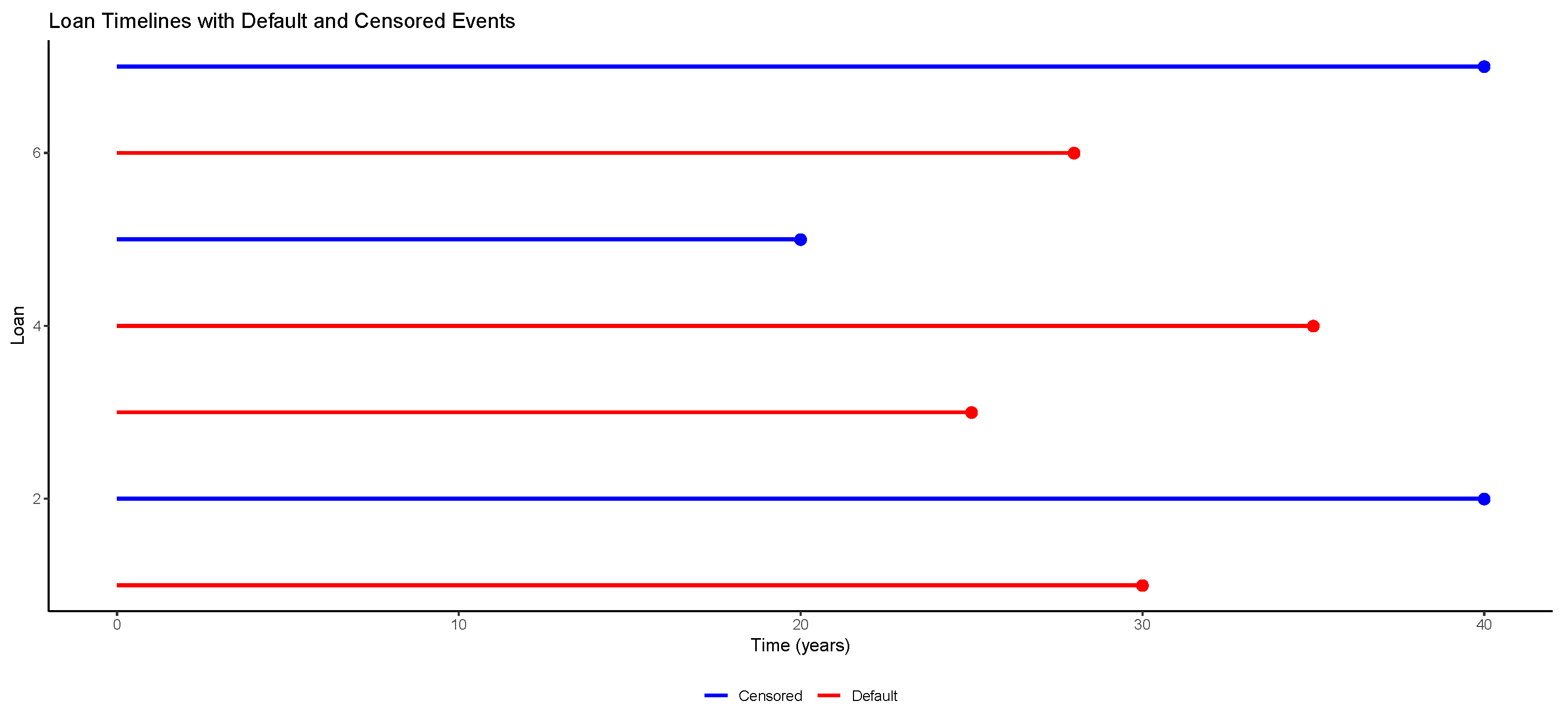
Figure 1. Loan timelines, indicating default and censored events.
Risks 13 00155 g001
Figure 2. Visual representation of the Survival Function ( S ( t ) ) and Hazard Rate ( h ( t ) ).
Risks 13 00155 g002
Figure 3. Estimated versus Calibrated Survival Probabilities.
Risks 13 00155 g003
Figure 4. Hazard function.
Risks 13 00155 g004
Figure 5. Probability density of default.
Risks 13 00155 g005
Figure 6. QQ-plot between estimated versus calibrated probabilities of default.
Risks 13 00155 g006
Figure 7. Number of loans at risk—estimated versus calibrated.
Risks 13 00155 g007
Figure 8. Number of defaults—estimated versus calibrated.
Risks 13 00155 g008
Figure 9. Simulated number of defaults.
Risks 13 00155 g009
Figure 10. Loss Given Default.
Risks 13 00155 g010
Figure 11. Loss processes.
Risks 13 00155 g011
Figure 12. Loss histograms.
Risks 13 00155 g012
Figure 13. 95% VaR and ES for the 4 LGD Scenarios, as a function of loan age.
Risks 13 00155 g013
Figure 14. Loss histograms per loan age for each scenario.
Risks 13 00155 g014
Table 1. Performance data of the portfolio.
Age Interval d j m j n j q ^ j s ^ j S ^ j
1[0, 1)0010,4790.0000001.0000001.000000
2[1, 2)21210,4790.0001910.9998090.999809
3[2, 3)3010,4650.0002870.9997130.999522
4[3, 4)32510,4620.0002870.9997130.999235
5[4, 5)42310,4340.0003840.9996160.998852
6[5, 6)8310,4070.0007690.9992310.998084
7[6, 7)92310,3960.0008670.9991330.997219
8[7, 8)8410,3640.0007720.9992280.996449
9[8, 9)9710,3520.0008700.9991300.995583
10[9, 10)94310,3360.0008730.9991270.994714
11[10, 11)111010,2840.0010700.9989300.993649
12[11, 12)92410,2630.0008780.9991220.992777
13[12, 13)137710,2300.0012760.9987240.991511
14[13, 14)126710,1400.0011870.9988130.990333
15[14, 15)121310,0610.0011930.9988070.989151
16[15, 16)135610,0360.0012990.9987010.987866
17[16, 17)15599670.0015050.9984950.986379
18[17, 18)20799470.0020110.9979890.984395
19[18, 19)23899200.0023190.9976810.982112
20[19, 20)22998890.0022260.9977740.979926
21[20, 21)242398580.0024370.9975630.977538
22[21, 22)25098110.0025480.9974520.975047
23[22, 23)24097860.0024520.9975480.972656
24[23, 24)27097620.0027660.9972340.969965
25[24, 25)301597350.0030840.9969160.966974
26[25, 26)335696900.0034150.9965850.963671
27[26, 27)3327596010.0034870.9965130.960311
28[27, 28)3710692930.0040040.9959960.956465
29[28, 29)3920091500.0043090.9956910.952344
30[29, 30)408589110.0045100.9954900.948048
31[30, 31)419887860.0046930.9953070.943599
32[31, 32)3910486470.0045380.9954620.939318
33[32, 33)3919885040.0046400.9953600.934959
34[33, 34)4315582670.0052510.9947490.930050
35[34, 35)5020080690.0062740.9937260.924215
36[35, 36)4925078190.0063690.9936310.918329
37[36, 37)5590075200.0077790.9922210.911185
38[37, 38)5445065650.0085170.9914830.903424
39[38, 39)55100060610.0098900.9901100.894489
40[39, 40)0500650060.0000001.0000000.894489
Based upon 10,479 real credit portfolios of 10 commercial banks observed over 40 years. All credits are of the same rating class and maturity equal to 40.
Table 2. Risk measures: VaR and ES.
Scenario 1Scenario 2Scenario 3Scenario 4
VaR
95%216,647.65422,462.92528,868.31981,093.91
99%217,283.22423,702.27536,135.021,035,259.28
ES
95%217,260.50423,657.97536,130.621,032,050.98
99%217,355.16423,842.57536,148.961,045,418.92
Table 3. VaR and ES per loans’ age, for each loss scenario.
Scenario 1 Scenario 2 Scenario 3 Scenario 4
AgeVaR 95ES 95VaR 99ES 99VaR 95ES 95VaR 99ES 99VaR 95ES 95VaR 99ES 99VaR 95ES 95VaR 99ES 99
158,50078,00078,00078,500292529252925292530,00030,50040,00040,5001500200020502150
295,000114,000114,000114,500975097509750975050,00060,00060,50070,0005000600065007000
3111,925129,500129,500129,55017,69617,84317,84320,47560,50070,00072,50075,000907510,50011,00012,500
4126,000166,500162,180180,00027,30027,30027,30028,08070,00092,50090,100100,00014,00018,50018,02020,000
5157,500179,375175,175192,50043,87543,87543,87544,36390,000102,500100,100110,00022,50025,62525,02527,500
6153,000178,500170,340204,00052,65052,65052,65052,65090,000105,000100,200120,00027,00031,50030,06036,000
7214,500239,250231,165247,50088,72588,72588,72588,725130,000145,000140,100150,00045,50050,75049,03552,500
8192,000216,000224,000255,00093,60093,60093,60094,380120,000135,000140,000145,00048,00054,00056,00057,500
9202,275232,500232,965279,000114,514114,953114,953122,850130,500150,000150,300180,00058,72567,50067,63581,000
10225,000240,000245,000250,000146,250146,250146,250146,250150,000160,000165,000170,00075,00080,00080,00090,000
11232,000253,750246,790275,500171,600171,600171,600171,600160,000175,000170,200190,00088,00096,25093,610104,500
12252,000266,000266,500266,750210,600210,600210,600211,770180,000190,000195,000200,000108,000114,000123,000150,000
13243,000265,500270,000275,000228,150228,150228,150228,150180,000196,667200,000240,000117,000127,833130,000160,000
14273,650299,000286,650351,000287,333288,015288,015300,300210,500230,000220,500270,000147,350161,000154,350189,000
15263,125285,000287,625300,000307,856308,588308,588321,750210,500228,000230,100240,000157,875171,000172,575180,000
16288,000324,000336,120348,000374,400374,400374,400375,960240,000270,000280,100290,000192,000216,000224,080232,000
17276,000296,125299,000305,000397,800397,800397,800397,800240,000257,500260,000270,000204,000218,875221,000235,000
18264,000302,500308,110319,000421,200421,200421,200424,710240,000275,000280,100290,000216,000247,500252,090261,000
19294,525317,100325,605336,000519,626520,553520,553537,225280,500302,000310,100320,000266,475286,900294,595304,000
20290,000315,000310,400350,000565,500565,500565,500567,450290,000315,000310,400350,000290,000315,000310,400350,000
21285,475317,300323,190342,000556,676539,078539,078557,603300,500334,000340,200360,000315,525350,700357,210378,000
22279,000301,500297,090306,000544,050544,050544,050544,050310,000335,000330,100340,000341,000368,500363,110374,000
23280,500312,375298,180365,500546,975546,975546,975546,975330,000367,500350,800430,000379,500422,625403,420494,500
24288,000300,000304,000335,000561,600561,600561,600563,160360,000375,000380,000390,000432,000450,000456,000500,000
25285,000296,250292,575300,000555,750555,750555,750555,750380,000395,000390,100400,000475,000493,750487,625500,000
26280,000294,000294,070301,000546,000546,000546,000547,365400,000420,000420,100430,000520,000546,000546,130559,000
27266,825289,900292,760318,500520,309519,675508,268508,268410,500446,000450,400490,000554,175602,100608,040661,500
28258,000285,000294,120306,000503,100503,100503,100504,270430,000475,000490,200510,000602,000665,000686,280714,000
29258,775275,000280,665297,000504,611505,148505,148514,800470,500500,000510,300540,000682,225725,000739,935783,000
30240,000261,250260,100270,000468,000468,000468,000470,925480,000522,500520,200540,000720,000783,750780,300810,000
31229,500243,000238,725261,000447,525447,525447,525448,403510,000540,000530,500580,000790,500837,000822,275899,000
32216,000223,000220,120232,000421,200421,200414,180421,200540,000557,500550,300580,000864,000892,000880,480928,000
33196,175208,600210,070217,000382,541382,883382,883390,390560,500596,000600,200620,000924,825983,400990,3301,023,000
34171,000182,000177,180195,000333,450333,450328,185333,450570,000606,667590,600650,000969,0001,031,3331,004,0201,105,000
35147,625155,500150,275177,500287,869288,113283,238288,113590,500622,000601,100710,0001,033,3751,088,5001,051,9251,242,500
36120,000122,667122,020124,000234,000234,000234,000234,000600,000613,333610,100620,0001,080,0001,104,0001,098,1801,116,000
3794,57598,70099,045103,500184,421184,568184,568187,493630,500658,000660,300690,0001,166,4251,217,3001,221,5551,276,500
3859,00062,50062,05067,000115,050115,050115,050115,245590,000625,000620,500670,0001,121,0001,187,5001,178,9501,273,000
3930,50033,00034,00034,00059,47559,47559,47559,475610,000660,000680,000690,0001,189,5001,287,0001,326,0001,357,000
Disclaimer/Publisher’s Note: The statements, opinions and data contained in all publications are solely those of the individual author(s) and contributor(s) and not of MDPI and/or the editor(s). MDPI and/or the editor(s) disclaim responsibility for any injury to people or property resulting from any ideas, methods, instructions or products referred to in the content.