Abstract
In this paper a new state model is introduced, an adaptative state model in a binary temporal representation (ASMBRT) as well as its application in constructing an algorithmic trading system. The presented model uses the binary temporal representation, which allows for a precise analysis of exchange rates without losing any informative value of the data. The basis of the model is the trajectory analysis for the ensuing changes in price quotations and dependencies between the duration of each change. The main advantage of the model is to eliminate the threshold analysis, used in existing state models. This solution allows for a more accurate identification of investor behavior patterns, which translates into a reduction of investment risk. In order to verify obtained results in practice, the paper presents a concept of creating an algorithmic trading system and an analysis of its financial effectiveness for the exchange rate most popular among investors, namely EUR/USD.
1. Introduction
Algorithmic trading systems are becoming increasingly popular among investors. Standard technical analysis methods often fail to effectively automate the decision-making process. Therefore, it is crucial to apply advanced methods of exchange rate modelling that enable estimation of the probability of the direction of future changes in the exchange rate trajectory (Dempster and Leemans 2006; Gallo and Fratello 2014; Liu et al. 2023). Standard technical analysis methods often fall short in effective automation of the decision-making process. Due to EU regulations that require brokers to disclose the percentage of clients incurring losses (ESMA 2018), approximately 70–80% of investors incur losses in the market for the most popular derivative instruments, i.e., CFD contracts (ESMA 2019; Andrade et al. 2025). This highlights a significant demand for new, advanced tools capable of estimating the probability of the price trends (Aldridge 2013; Dempster and Leemans 2006; Liu et al. 2023). These tools should be as independent as possible from specific parameters that change the system’s operation over time, which is particularly important in risk calculation are observed.
The study of predictive methods based on technical analysis in financial markets has a very long history. For many years—and even today—many investors continue to use visual techniques such as pattern recognition or trendline drawing. However, these oldest and most basic forms of technical analysis rely heavily on the analyst’s subjective interpretation, which makes them impossible to verify using typical scientific methods—an example can be Elliott Wave analysis (Frost and Prechter 2005).
Among the more popular and verifiable technical analysis tools are those based on indicators such as moving averages, RSI, MACD, etc. (Cohen 2021; Sukma and Namahoot 2024). This research direction is the subject of many current papers, but the number of possible model parameter combinations, trade entry rules based on indicators, and similar variables is so vast that comprehensive verification is currently unfeasible.
Another prominent group consists of the increasingly popular studies using machine learning techniques (Sezer and Ozbayoglu 2018; Théate and Ernst 2021). Despite many promising results, these methods—although highly popular in recent years—have not contributed to any noticeable change in the statistics on investor losses (ESMA 2019; Andrade et al. 2025). This may indirectly cast doubt on the revolutionary nature of such techniques.
The final group includes various proprietary modeling approaches that apply original analytical concepts. One example is price modeling using a binary–temporal representation (Stasiak et al. 2025). The research presented in this article belongs to this particular stream.
The general majority of investors and researchers use the candlestick chart representation to analyze exchange rate trajectories (Rundo et al. 2019). Most of the standard methods of technical analysis are also based on the candlestick charts (Schlossberg 2006). Using this kind of representation leads to the loss of important information about the exchange rate trajectory ‘inside the candle’. In the case of analyzing very short exchange rate changes of a small range, this kind of information loss can result in the falsification of research results. The consequences of using candlestick chart representation are described in detail in (Stasiak 2020). The binary-temporal representation can be understood as an alternative to the candlestick representation, since its construction does not result in a drop in the informative value of the data (greater than an assumed level).
The article presents a new concept of an adaptive state model of the binary-temporal representation (ASMBTR), which allows for an approximation of the probability of the direction of future changes in the exchange rate with higher precision than the state model of the binary-temporal representation (SMBTR) (Stasiak et al. 2025). Research presented in this paper was conducted based on historical data on EUR/USD currency pair—the most traded pair among retail investors.
The paper is structured as follows: after a brief introduction, Section 2 outlines the concept of binary-temporal representation and its use in state modelling. Section 3 presents the SMBTR model along with the newly proposed ASMBTR model. Section 4 describes the architecture of an algorithmic trading system based on ASMBTR and evaluates its performance using the EUR/USD pair. The paper concludes with a summary of the findings.
2. Binary-Temporal Representation
The vast majority of investors and researchers use candlestick representation for their research data (Kirkpatrick and Dahlquist 2010; Chen and Tsai 2020). In this kind of representation, for a given timeframe (e.g., an hour), the changes in exchange rates are described by four parameters: maximal, minimal, opening, and closing price. Moreover, a lot of smaller changes have the character of random fluctuations (Lo et al. 2000; Neely and Weller 2011). As a consequence, analysis of such big and noisy data is hard and often impossible due to the time restriction The smallest time interval usually used is one minute. Using this kind of representation, even with such a short time frame, can lead to a significant loss of information about the changes that took place within the candlestick timeframe since the exchange rate trajectory can change multiple times inside the candle. As a consequence, such loss can result in faulty modelling and wrong decisions made by an algorithmic trade system constructed based on such representation (Stasiak 2020).
Of course, the exchange rate trajectory can be analyzed with the use of unprocessed tick data, that is, data that include all possible changes in the trajectory. However, because of the high frequency of changes in the tick data, information about the exchange rate can take up a lot of space in the computer memory (even a few GB for a one-year observation period). Moreover, a lot of smaller changes have the character of random fluctuations. As a consequence, analysis of such large and noisy data is hard and often impossible due to time restriction.
The binary-temporal representation, which was inspired by the point-symbolic method (De Villiers 1933), eliminates the disadvantages of the candlestick charts. In binary-temporal representation, each exchange rate change of a given value (i.e., so-called discretization unit) is assigned two parameters: the corresponding binary value ε (ε = 1 for exchange rate increase, ε = 0 for a drop) and the duration of the change in seconds, denoted as t. Figure 1 presents an example of the realization of the binary-temporal representation (Stasiak 2020).

Figure 1.
An example of a binary-temporal representation. Source: Author.
Thus, a given time period consisting of N changes can be described by following change series :
where and are the binary value and the duration of i-th change .
An important characteristic of the binary-temporal representation is registering all changes of the value higher (or equal) to the discretization unit. This means that we are sure that no significant changes will be omitted from the exchange rate analysis.
The form and properties of the binary-temporal representation are dependent on the assumed discretization unit. Appointing a too small discretization unit can result in registering changes that would usually be considered noise; on the other hand, assigning too big discretization unit leads to a loss of significant information about the character of the exchange rate changes. In (Stasiak and Staszak 2024) the method described allows for a statistical analysis of a binary-temporal representation, used for appointing proper discretization units.
At the foundation of the technical analysis lies the conviction that investors make decisions according to some describable and repetitive patterns. Theories of Dow and Elliott (Frost and Prechter 2005) also assume repetitiveness of behaviors. This assumption can be justified by behavioral research (psychology (Oberlechner 2005)) or statistical research (statistical tests (Stasiak and Staszak 2024)). Statistical research indicates that the price of financial instruments in the binary-temporal representation, for properly appointed discretization units, is not random. To predict the direction of changes, we can use state modelling. The main goal of state modelling in a binary-temporal representation is the identification of those kinds of patterns and defining the probability of their occurrence. As a result, we statistically identify patterns of behaviors that are observable more often and can be used in the future as signals in automatic trade systems (Stasiak et al. 2025).
3. Adaptive State Model of a Binary-Temporal Representation
Let us now consider a State Model of a Binary-Temporal Representation (SMBTR). The model operates on 3 parameters: number of analyzed changes m and the number of previous changes n, in which the time threshold is considered. The model can be described in the Binary-temporal State Model BTSM (m,n,) notation. The state in this model, i.e., , is defined as a pair of elements, first being m previous changes denoted binarily by in the binary-temporal representation; the second one is the series of n binary values , showing if the duration of a given change is greater or smaller than the threshold :
where describes the duration of the i-th change, .
The state space Ω can be described as:
Let us now consider an example of the SMBTR (2, 1, 120) model. In this model, we analyze two previous changes (m = 2) in a binary-temporal representation and the duration of the last change (n = 1). Let us assume that = {0,345}, which means that the i-th (current) change corresponds to a drop of the size of one discretization unit in the time period of 345 s. Let us assume further that the = {1,45}, i.e., (i − 1)-th (previous) change corresponds to an increase of the size of one discretization unit in a 45-s time period. This means that the market is actually in a state (10;1), since last two changes consist of an increase and a decrease in the course trajectory, where the last change lasted more than 120 s. Let us now consider a situation, where another change occurs, = {1,78}; the market now transitions into the state (01;0).
The visualization of the SMBTR is presented as a state diagram in Figure 2, showing transitions between states for the considered SMBTR (2, 1, 120) model.
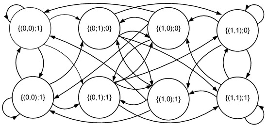
Figure 2.
State diagram for the SMBTR (2, 1, 120) model.
The form of the state diagram is dependent on parameters m and n, and edges are assigned the frequency of transitions, appointed from the historical data and assumed time threshold . The transition frequencies (denoted P[(state 1)→(state 2)]) can be interpreted as probability estimators for the transitions between states. In order to use the model in investment decision-making practice, we need to assess the probability of the future change in the direction of the exchange rate. By simulating particular transition probabilities, we can determine the probability distribution of the next change in the exchange rate trajectory. In Table 1 we can see this kind of distribution for the SMBTR (2, 1, 15,000) model, calculated for the EUR/USD exchange rate with 50 pips discretization units, considered in a two-year time period (1 January 2020–1 January 2022). Based on this distribution, we can create a prediction table (Table 2), which stands as a base to parametrization of automatic trade systems: after the detection of a particular state, we can make a transaction corresponding to the more probable direction of the next forecasted change.

Table 1.
Probability distribution of the direction of the exchange rate change in the SMBTR (2, 1, 15,000) model.
Table 2.
Prediction table calculated based on the SMBTR (2, 1, 120) model.
The presented model has one particular disadvantage: the time threshold parameter is appointed arbitrarily. That leads to the question if the approach is justified: the observed dependencies between fixed threshold and the distribution of the future change direction can differ in time—i.e., the threshold value can have a different impact on the distribution in time. The answer to this problem is the proposition of the adaptive SMBTR model (ASMBTR), which analyses the dependencies between the duration of the current and previous change in exchange rate trajectory. This kind of approach allows for a better description of the behaviour patterns of the investors, which are unquestionably correlated with the frequency of changes registered on the market in the binary-temporal representation. In the ASMBTR model we assume that the series of n binary values are appointed based on a direct comparison between the duration of the subsequent changes:
Equation (4) changes the whole concept of modelling, since it eliminates the threshold parameter and replaces the comparison of the ensuing change durations with the threshold time by a direct comparison between the ensuing changes. In the new ABTSM model, parameters m and n are defined analogously to the SMBTR model, and thus can be denoted as ASMBTR (m,n). The state () is also described in the same way as in the SMBTR model. As a consequence, the number of states and the transition diagram in both models are identical.
Let us now consider an example of the operation of the ASMBTR (2,1) model. In this case we analyze two previous changes (m = 2) in the binary-temporal representation, and we analyze the duration of the last change (n = 1). Let us assume that = {0,345}, which means that the i-th change corresponds to the drop of the size of one discretization unit in the time period of 345 s. Let us further assume further that = {1,45}, so that (i − 1)-th change corresponds to an increase of the size of one discretization unit in the duration of 45 s. This means that the market finds itself in the state (10;1), since two previous changes were an increase and a decrease, the last lasting longer than the previous (345 > 45). If another change occurs, for example = {1,78}, the course will reach the state (01;0), since 78 < 345.
Based on the model parameters (m and n) and the analysis of historical data, we can construct a proper state diagram. This diagram, as mentioned before, will take the form of a weighted graph and has an identical structure as the diagram in the BTSM model. The differences are visible only in the probability estimators of particular transitions between states.
4. Construction of an Algorithmic Trading System Based on the SMBTR and ASMBTR Models
The concept of constructing algorithmic trade systems based on state modelling of the exchange rate in a binary-temporal representation is very simple. The changes in exchange rate trajectory in the binary-temporal representation correspond to single transactions. If we can deduce from the prediction table that the more probable change corresponds to an increase in the exchange rate, we buy, if contrary—we sell. At the end of the change, the transaction is closed—with a revenue, if the prediction was correct, or with a loss if the prediction was wrong.
The process of constructing and evaluating the effectiveness of the system assumes generation of a prediction table based on a time period appointed beforehand, with historical data. Conducting a backtest of the performance of the system in the ensuing time period with historical data allows for the evaluation of the financial effectiveness of the system.
In case of the algorithmic trade systems that are based on the leveraged financial instruments such as CFD contracts for currencies—to assess the effectiveness one has to consider indicators that are based on analyzing the drawdown. Such indicators are Calmar’s, Sterling and Burke’s indicators (Aldridge 2013; Nystrup et al. 2019). The most popular is the Calmar’s indicator (Young 1991; Pardo 2011), which is defined as the ratio between the average annual return rate () dimnished by the return rate free of risk (), to the maximal drawdown (mdd) registered during the backtest:
In case of analyzing the algorithmic trade systems that are based on CFD contracts, there exists no return rate that is free of risk, so we assume that . In further research we used this indicator in order to analyse obtained backtests results for the algorithmic trade systems and selection of optimal parameters.
5. Analysis of the Effectiveness of State Modeling Based on ASMBTR and SMBTR Models
To evaluate the capabilities of the two models, a parameter optimization process and a financial effectiveness assessment were conducted. The study was based on historical tick data that span the period from 1 January 2019 to 1 January 2024. The data comes from Ducascopy broker platform. The data set was divided into three periods: training (1 January 2019–1 January 2021), validation (1 January 2021–1 January 2023), and testing (1 January 2023–1 January 2024), during which the final results were verified.
Consider the evaluation of the ASMBTR model. In the first step, a prediction table was generated based on the training period. This was followed by a backtest of an algorithmic trading system using the prediction table for the validation period. This process was repeated for all discretization units in which the instrument’s price maintained its informational value. The range of valid discretization units was determined using NIST statistical tests (Rukhin et al. 2010), with the exact procedure of verification of Fama’s Market Efficiency Hypothesis (Fama 1970) described in (Stasiak and Staszak 2024). The model was tested for values of the parameter m ranging from 1 to 4. Subsequently, the optimal value of m and the discretization unit that yielded the highest backtest performance—measured using the Calmar ratio—were selected. Then a final backtest was then conducted on the test set using these parameters to confirm the model’s utility.
To compare the effectiveness of the ASMBTR model with the SMBTR model, the time threshold that yielded the highest algorithmic trading performance during the validation period—using the optimal discretization unit and the m parameter identified for ASMBTR—was selected. All possible combinations of time thresholds (from 30 s to 540,321 s—the longest observed change), in increments of 5-s, were verified. A final backtest was performed in the test period for the selected threshold to confirm the effectiveness of the system.
The analysis showed that the most effective system was the ASMBTR (2,1) based system for a 77-pips discretization unit. In Table 3 we can see the prediction results obtained thanks to the modelling.
Table 3.
Prediction table for ASMBTR (2,1) with a 77-pip discretization unit.
In Figure 3, the results of the backtest conducted during the validation period are presented. In this period, the backtest of the system is characterized by a Calmar ratio of 1.0115. Next, in order to confirm the effectiveness of the system, a backtest was carried out during a one-year testing period. In Figure 4 we can see the backtest results for this system. In this period, the system backtest is characterized by a Calmar ratio of 0.4146. In the testing period, therefore, the effectiveness of the system decreased significantly, although it should be emphasized that the system still generates a positive rate of return—the trend line still indicates an upward tendency.
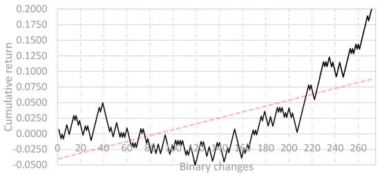
Figure 3.
Backtest results (with trend line) for the algorithmic trading system based on the ASMBTR(2;1) model—validation period. Source: Authors.
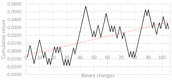
Figure 4.
Backtest results (with trend line) for the algorithmic trading system based on the ASMBTR(2,1) model—test period. Source: Authors.
Consider the analysis and selection of parameters for a system based on the SMBTR model. The most financially efficient algorithmic trading system was developed using the SMBTR (2, 2, 175,170) model with a 77-pip discretization unit. The prediction table is presented in Table 4.
Table 4.
Prediction table for the SMBTR (2, 2, 175,170) model with a 77-pip discretization unit calculated for the EUR/USD exchange rate.
In Figure 5, the results of the backtest conducted during the validation period are presented. In this period, the system backtestis characterized by a Calmar ratio of 1.1512. Next, in order to confirm the effectiveness of the system, a backtest was carried out during a testing period of one year. In Figure 6 we can see the backtest results for this system. In this period, the backtest of the system is characterized by a Calmar ratio of 0.3340. In the testing period, therefore, the effectiveness of the system decreased significantly, although it should be emphasized that the system still generates a positive rate of return, the trend line still indicates an upward tendency.

Figure 5.
Backtest results (with trend line) for the algorithmic trading system based on the SMBTR (2, 2, 175,170) model—validation period. Source: Authors.
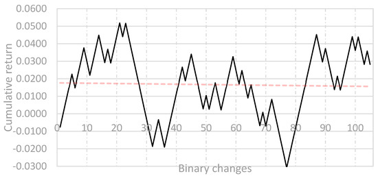
Figure 6.
Backtest results (with trend line) for the algorithmic trading system based on the SMBTR (2, 2, 175,170) model—test period. Source: Author.
6. Discussion
The backtest results of both strategies based on the SMBTR and ASMBTR models exhibit a similar pattern in terms of return dynamics during the validation period. In both cases, a decrease in effectiveness was observed during the test period; however, the performance remained positive (Calmar ratio > 0). On the one hand, this result can be seen as confirmation of the effectiveness of the modeling approach; on the other hand, the drop in performance indicates significant variability in strategy effectiveness. Attention should also be paid to the trend in return rates—in the case of the system built using the ASMBTR model, this trend is upward.
Despite the small difference, it is worth highlighting that the ASMBTR model does not require setting a specific time threshold value. This approach makes the model more resistant to the phenomenon of overfitting, i.e., excessive adaptation of the model to historical data. Overfitting is an undesirable effect, as it tends to produce very good results but only in the short term (Aparicio and López de Prado 2018). In the context of designing algorithmic trading systems (for which it is not possible to conduct a reliable risk analysis—these systems at some point begin to generate unforeseen losses, leading to the investor’s bankruptcy). Therefore, it should be concluded that even with a slight difference in effectiveness, using systems based on the ASMBTR model is more advisable.
In the case of the proposed systems, certain concerns may arise regarding the use of rarely occurring states as trading signals. On the one hand, one might argue that it is not possible to confirm their statistical significance; on the other hand, it can be assumed that these states indicate very specific—though rare—patterns of investor behavior, which are characterized by a high predictive potential. The Author adopted the latter reasoning, deciding not to apply any selection or filtering of these states.
It is also worth noting that this issue primarily concerns the SMBTR model. In the case of the ASMBTR model, the distribution of state occurrences appears to be more uniform. Based on the presented analysis, a key conclusion can be drawn—in the analysis of investor behavior patterns, temporal dependency analysis yields comparable or even better results than threshold-based analysis. This conclusion is highly relevant for further research and the construction of new models, in which replacing threshold analysis with dependency analysis between successive changes can drastically reduce the number of parameters.
The presented ASMBTR model was compared with the generally accepted methodology (including a division into training and validation periods) and validated using the most accurate backtesting method available—forward testing on tick-level data. A multi-year time horizon was also used in the analysis, which aligns with established standards. Financial performance was measured using the Calmar ratio, a practical metric specifically designed for systems based on derivative instruments.
A precise comparison of results with models presented in other studies proves difficult, as many papers demonstrate their proposed methods on different financial instruments or over different time periods. Moreover, the Calmar ratio itself is often calculated differently across studies—for instance, using total return instead of annualized return (Dunis et al. 2008). Many studies also replace the Calmar ratio with purely statistical backtest evaluation metrics such as MAE, RMSE, or MAPE, which are not appropriate for analyzing leveraged instruments, where investor risk is better represented by drawdowns.
It is important to emphasize the universality of the modeling approach proposed in the article. The modeling and optimization results of the algorithmic trading systems were illustrated using the EUR/USD currency pair due to its popularity among investors. However, the same process can be applied to any financial instrument, provided that the specific characteristics of the given market are taken into account. For example, the EUR/USD market is known for its exceptional liquidity, while CFD contracts on currency pairs from the “exotic” basket may experience low liquidity in certain periods, which could result in the failure to execute some trades.
7. Conclusions
In the paper, we present a new model, the Adaptive State Model in a Binary Temporal Representation (ASMBTR). This model differs from the standard SMBTR model in its method of analysing the duration of changes in exchange rate trajectories within the binary-temporal framework. In the model, an analysis of the dependencies between change times was used instead of threshold analysis (as in the case of the standard SMBTR model). This concept allows the analysis to be independent of the specific parameter values, thereby eliminating the possibility of overfitting.
The effects of state modelling in the binary-temporal representation can be easily implemented in algorithmic trading systems. Therefore, the article presents the results of empirical studies for the most popular currency pair among investors, EUR/USD. The study identified the most financially effective system based on the SMBTR and ASMBTR models. The results were then compared in terms of financial effectiveness. The findings indicated that the most effective system, characterized by a Calmar ratio of 0.4146, was obtained based on the ASMBTR model. It should be emphasized that replacing threshold analysis reduces the investor’s risk borne by changes in market conditions causing a suboptimal selection of time thresholds.
The presented results demonstrate that the ASMBTR model can serve as a foundation for the construction of an effective algorithmic trading systems with a positive return rate. The obtained results confirm the validity of replacing threshold analysis with an analysis of mutual temporal dependencies in state modelling. It is crucial to highlight that the proposed model has a universal character and can be applied to the analysis of any financial instrument, including Forex, metals, etc.
Funding
This research received no external funding.
Data Availability Statement
Data sharing is not applicable (only appropriate if no new data is generated or the article describes entirely theoretical research).
Conflicts of Interest
The authors declare no conflict of interest.
References
- Aldridge, Irene. 2013. High-Frequency Trading: A Practical Guide to Algorithmic Strategies and Trading Systems. Hoboken: Wiley. [Google Scholar]
- Andrade, Marco, Daniel Costa, Liat Weiss-Cohen, Jack Torrance, and Philip Newall. 2025. Trading Is a Losing Game: An Audit of Deceptive Choice Architecture in Demo-Mode Contract for Difference (CFD) Trading Apps. Behavioural Public Policy 1: 1–23. [Google Scholar] [CrossRef]
- Aparicio, Daniel, and Marcos López de Prado. 2018. How Hard Is It to Pick the Right Model? MCS and Backtest Overfitting. Algorithmic Finance 7: 53–61. [Google Scholar] [CrossRef]
- Chen, Jui-Hsien, and Yu-Chuan Tsai. 2020. Encoding Candlesticks as Images for Pattern Classification Using Convolutional Neural Networks. Financial Innovation 6: 26. [Google Scholar] [CrossRef]
- Cohen, Gil. 2021. Optimizing algorithmic strategies for trading bitcoin. Computational Economics 57: 639–54. [Google Scholar] [CrossRef]
- Dempster, Michael, and Vasco Leemans. 2006. An automated FX trading system using adaptive reinforcement learning. Expert Systems with Applications 30: 543–52. [Google Scholar] [CrossRef]
- De Villiers, Victor. 1933. The Point and Figure Method of Anticipating Stock Price Movements Complete Theory & Practice. A Reprint of the 1933 Edition including a chart on the 1929 crash. New York: Windsor Books. [Google Scholar]
- Dunis, Christian, Jason Laws, and Ben Evans. 2008. Trading futures spread portfolios: Applications of higher order and recurrent networks. The European Journal of Finance 14: 503–21. [Google Scholar] [CrossRef]
- European Securities and Markets Authority (ESMA). 2018. ESMA Adopts Final Product Intervention Measures on CFDs and Binary Options. Available online: https://www.esma.europa.eu (accessed on 12 July 2025).
- European Securities and Markets Authority (ESMA). 2019. Notice of ESMA’s Product Intervention Renewal Decision in Relation to Contracts for Differences. Available online: https://www.esma.europa.eu/sites/default/files/library/esma35-43-1912_cfd_renewal_3_-_notice_en.pdf (accessed on 12 July 2025).
- Fama, Eugene. 1970. Efficient Capital Markets. Journal of Finance 25: 383–417. [Google Scholar] [CrossRef]
- Frost, Alfred John, and Robert Rougelot Prechter. 2005. Elliott Wave Principle: Key to Market Behavior. Gainesville: New Classics Library. [Google Scholar]
- Gallo, Crescenzio, and Angelo Fratello. 2014. The Forex Market in Practice: A Computing Approach for Automated Trading Strategies. International Journal of Economics & Management Sciences 3: 1000169. [Google Scholar] [CrossRef]
- Kirkpatrick, Charles, and Julie Dahlquist. 2010. Technical Analysis: The Complete Resource for Financial Market Technicians, 2nd ed. Upper Saddle River: FT Press. [Google Scholar]
- Liu, Peipei, Yunfeng Zhang, Fangxun Bao, Xunxiang Yao, and Caiming Zhang. 2023. Multi-type data fusion framework based on deep reinforcement learning for algorithmic trading. Applied Intelligence 53: 1683–706. [Google Scholar] [CrossRef]
- Lo, Andrew W., Harry Mamaysky, and Jiang Wang. 2000. Foundations of Technical Analysis: Computational Algorithms, Statistical Inference, and Empirical Implementation. The Journal of Finance 55: 1705–65. [Google Scholar] [CrossRef]
- Neely, Christopher J., and Paul A. Weller. 2011. Technical Analysis in the Foreign Exchange Market. Federal Reserve Bank of St. Louis Working Paper. St. Louis: Federal Reserve Bank of St. Louis. [Google Scholar]
- Nystrup, Peter, Stephen Boyd, Erik Lindström, and Henrik Madsen. 2019. Multi-Period Portfolio Selection with Drawdown Control. Annals of Operations Research 282: 245–71. [Google Scholar] [CrossRef]
- Oberlechner, Thomas. 2005. The Psychology of the Foreign Exchange Market. Hoboken: John Wiley & Sons. [Google Scholar]
- Pardo, Robert. 2011. The Evaluation and Optimization of Trading Strategies. Hoboken: John Wiley & Sons. [Google Scholar]
- Rukhin, Andrew, Juan Soto, James Nechvatal, Miles Smid, Elaine Barker, Stefan Leigh, Mark Levenson, Mark Vangel, David Banks, Alan Heckert, and et al. 2010. Statistical Test Suite for Random and Pseudorandom Number Generators for Cryptographic Applications. NIST Special Publication 800-22. Gaithersburg: National Institute of Standards and Technology. [Google Scholar]
- Rundo, Francesco, Francesca Trenta, Agatino Luigi di Stallo, and Sebastiano Battiato. 2019. Grid Trading System Robot (GTSbot): A Novel Mathematical Algorithm for Trading FX Market. Applied Sciences 9: 1796. [Google Scholar] [CrossRef]
- Schlossberg, Boris. 2006. Technical Analysis of the Currency Market: Classic Techniques for Profiting from Market Swings and Trader Sentiment. Hoboken: John Wiley & Sons, Inc. [Google Scholar] [CrossRef]
- Sezer, Omer Berat, and Ahmet Murat Ozbayoglu. 2018. Algorithmic financial trading with deep convolutional neural networks: Time series to image conversion approach. Applied Soft Computing 70: 525–38. [Google Scholar] [CrossRef]
- Stasak, Michał Dominik. 2020. Candlestick—The Main Mistake of Economy Research in High-Frequency Markets. International Journal of Financial Studies 8: 59. [Google Scholar] [CrossRef]
- Stasiak, Michał Dominik, and Żaneta Staszak. 2024. Are Changes in Crude Oil Prices Predictable? In Sustainable Global Economic Development within 2025 Vision: Research and Practice. Paper presented at 43rd International Business Information Management Association Conference (IBIMA), Granada, Spain, November 27–28; Edited by Khalid Soliman. King of Prussia: IBIMA Publishing LLC. [Google Scholar]
- Stasiak, Michał Dominik, Żaneta Staszak, Joanna Siwek, and Dominik Wojcieszak. 2025. Application of State Models in a Binary–Temporal Representation for the Prediction and Modelling of Crude Oil Prices. Energies 18: 691. [Google Scholar] [CrossRef]
- Sukma, Niken, and Chaiporn Namahoot. 2024. Enhancing trading strategies: A multi-indicator analysis for profitable algorithmic trading. Computational Economics 65: 3807–40. [Google Scholar] [CrossRef]
- Théate, Thibaut, and Damien Ernst. 2021. An application of deep reinforcement learning to algorithmic trading. Expert Systems with Applications 173: 114632. [Google Scholar] [CrossRef]
- Young, Terry. 1991. Calmar ratio: A smoother tool. Futures 20: 40. [Google Scholar]


Disclaimer/Publisher’s Note: The statements, opinions and data contained in all publications are solely those of the individual author(s) and contributor(s) and not of MDPI and/or the editor(s). MDPI and/or the editor(s) disclaim responsibility for any injury to people or property resulting from any ideas, methods, instructions or products referred to in the content. |
© 2025 by the author. Licensee MDPI, Basel, Switzerland. This article is an open access article distributed under the terms and conditions of the Creative Commons Attribution (CC BY) license (https://creativecommons.org/licenses/by/4.0/).