Volatility Modeling and Tail Risk Estimation of Financial Assets: Evidence from Gold, Oil, Bitcoin, and Stocks for Selected Markets

Abstract

As investment portfolios become increasingly diversified and financial asset risks grow more complex, accurately forecasting the risk of multiple asset classes through mathematical modeling and identifying their heterogeneity has emerged as a critical topic in financial research. This study examines the volatility and tail risk of gold, crude oil, Bitcoin, and selected stock markets. Methodologically, we propose two improved Value at Risk (VaR) forecasting models that combine the autoregressive (AR) model, Exponential Generalized Autoregressive Conditional Heteroskedasticity (EGARCH) model, Extreme Value Theory (EVT), skewed heavy-tailed distributions, and a rolling window estimation approach. The model’s performance is evaluated using the Kupiec test and the Christoffersen test, both of which indicate that traditional VaR models have become inadequate under current complex risk conditions. The proposed models demonstrate superior accuracy in predicting VaR and are applicable to a wide range of financial assets. Empirical results reveal that Bitcoin and the Chinese stock market exhibit no leverage effect, indicating distinct risk profiles. Among the assets analyzed, Bitcoin and crude oil are associated with the highest levels of risk, gold with the lowest, and stock markets occupy an intermediate position. The findings offer practical implications for asset allocation and policy design.

1. Introduction

Against the backdrop of rapid technological advancement and ongoing financial market liberalization, investors’ asset allocation behavior has undergone a profound transformation. To enhance portfolio risk resilience and return efficiency, investors are increasingly inclined to incorporate a broader range of financial instruments—including foreign equities, commodities, and digital assets—into their investment portfolios. The traditional strategy centered on domestic equities is gradually being replaced by diversified allocations across markets and asset classes (He 2021; Kupabado and Kaehler 2025; Yang et al. 2023). In recent years, the hedging and safe-haven properties of oil and gold have become more prominent. With the expansion of derivatives markets and the widespread use of exchange-traded funds, these commodities have experienced significant improvements in liquidity and price discovery efficiency, accelerating their transition into standardized financial investment instruments (Chincarini and Moneta 2021; Kang et al. 2023). Meanwhile, Bitcoin, as a representative cryptocurrency, has gradually gained recognition as a potential digital safe-haven asset and hedge against inflation due to its decentralized architecture and fixed supply (Blau et al. 2021; Krause 2024). In this context of increasingly diversified portfolios, the share of oil, gold, and Bitcoin in asset allocations has grown steadily, and the evolving risk profiles of these assets have drawn considerable attention from both investors and academia.

Since the global financial crisis of 2008, the frequent occurrence of major events such as the COVID-19 pandemic and geopolitical conflicts has led to rapid and complex shifts in financial asset risk levels. These changes have rendered traditional risk assessment methods increasingly inadequate for forecasting market risks, thereby complicating investment decision-making and presenting major challenges for policymakers in terms of market intervention, regulatory response, and macroeconomic stabilization (Boonman 2023; Díaz et al. 2022). In light of these developments, constructing mathematical models capable of forecasting risks across multiple asset classes and analyzing the heterogeneity of asset-specific risk features has become essential. Such models can enhance investors’ risk warning capabilities, improve the efficiency of asset allocation, and support the formulation of policies aimed at safeguarding financial stability.

Although empirical research on financial asset risk has made notable progress, several limitations remain. First, most existing studies concentrate on a single asset class, lacking a unified econometric framework for the systematic comparison and integrated assessment of risks across diverse financial assets such as gold, crude oil, Bitcoin, and various types of equities. This limitation constrains the applicability of current findings to diversified portfolio risk management. Second, the literature predominantly emphasizes return-based analyses, while studies focusing on tail risk remain insufficient (Das et al. 2023; Patra 2021). This tendency may understate the vulnerability of financial markets under extreme conditions. Third, although VaR modeling techniques have evolved in recent years, and some have demonstrated improved predictive performance, most models are still tailored to specific asset categories and lack the generalizability needed for multi-asset risk forecasting (Likitratcharoen and Suwannamalik 2024).

To address the limitations identified in the existing literature, this study investigates the risk characteristics of gold, crude oil, Bitcoin, and equity markets within a unified analytical framework, aiming to conduct a systematic comparison across asset classes. Given that stock market risk is significantly influenced by the level of economic development, this study follows the MSCI global equity market classification and selects four representative stock markets from both developed and emerging economies based on market capitalization rankings, with the goal of revealing the heterogeneity in risk across different economic systems (Bekaert et al. 2023). Methodologically, an AR–EGARCH model is first constructed to capture and compare the volatility patterns and their heterogeneity across the selected assets. For tail risk estimation, two novel models are proposed: the AR–EGARCH–VaR model and the AR–EGARCH–EVT–VaR model, both incorporating rolling window estimation and skewed heavy-tailed distributions. These two improved models are evaluated against three benchmark approaches—historical simulation, Monte Carlo simulation, and the standard GARCH–VaR model. The comparative performance is assessed using the Kupiec unconditional coverage test and the Christoffersen conditional coverage test, providing evidence of each model’s predictive accuracy across asset types. Based on the empirical results, the most effective AR–EGARCH–VaR model is then applied to conduct a detailed comparison of tail risks, highlighting structural differences in tail risk across asset classes.

The innovations and contributions of this study are threefold. First, in terms of methodology, it integrates rolling window techniques with AR model, EGARCH model, EVT, and skewed heavy-tailed distributions to construct two enhanced VaR forecasting models: AR–EGARCH–VaR and AR–EGARCH–EVT–VaR. These models substantially improve the precision and applicability of tail risk prediction across multiple assets. Second, in terms of risk assessment, this study considers both volatility and tail risk dimensions, moving beyond the single-risk-metric focus prevalent in prior studies. This allows for a multidimensional framework for cross-asset risk comparison. Third, in terms of application scope, the proposed VaR modeling framework is extended to include non-traditional financial assets such as gold, crude oil, and Bitcoin, alongside equities from both developed and emerging markets. This approach addresses the gap in the literature concerning unified tail risk modeling across diverse asset classes.

This research holds both theoretical and practical significance. From a theoretical perspective, it evaluates the risk profiles of various representative financial assets within a consistent econometric framework and from multiple analytical angles. The findings uncover structural differences in risk characteristics across asset types, enriching the perspective of comparative risk analysis. Moreover, the improved VaR models demonstrate superior predictive performance across different asset classes and exhibit strong cross-asset adaptability, offering theoretical support for the generalizability of tail risk measurement methods. On a practical level, for investors, the enhanced models provide more accurate forecasts of asset-specific tail risks, facilitating better risk exposure management and more stable returns. The empirical insights into the differentiated risk profiles also offer valuable guidance for constructing resilient investment portfolios. For regulatory bodies, the proposed VaR models can support the development of comprehensive multi-asset risk monitoring and early warning systems and assist in identifying potential sources of systemic risk. Furthermore, the dynamic characterization of asset volatility and tail risk can inform crisis-time market risk assessment, enabling more effective macroprudential policies and enhancing regulatory foresight.

The remainder of this paper is organized as follows. Section 2 provides a literature review, summarizing recent advances in multi-asset risk modeling and identifying key research gaps. Section 3 introduces the data and methodology, detailing variable selection and the theoretical foundations of the models employed. Section 4 presents the empirical findings, analyzes the risk profiles of different assets, and evaluates the performance of the proposed models. Section 5 concludes with a summary of the main results and offers policy recommendations.

2. Literature Review

2.1. Risk Characteristics of Financial Assets

In recent years, escalating global economic volatility and increasing uncertainty in financial markets have drawn growing academic attention to the risk performance and safe-haven properties of diversified financial assets under various crisis conditions. Assets such as gold, Bitcoin, crude oil, and major global equity markets have become focal points in international finance research due to their central roles in the financial system and the highly heterogeneous nature of their risk profiles (Yen-Ku et al. 2022; Tanin et al. 2022). Against this backdrop, empirical studies on different asset classes have proliferated, providing insights into their risk characteristics and behavior during financial crises. This section reviews key developments and empirical findings in the literature concerning the risk features and crisis-time performance of these assets.

2.1.1. Risk Features and Performance of Non-Equity Assets

Among the studies centered on gold, researchers have primarily analyzed its risk behavior over different historical periods to assess its efficacy as a safe-haven asset. Most findings indicate that gold exhibits relatively low risk and serves as a significant crisis hedge. For example, Gomis-Porqueras et al. (2022) examined extreme price fluctuations of gold during the European sovereign debt crisis, stock market crashes, and oil price shocks. Their results confirmed that gold’s extreme price movements remained relatively stable during these episodes, validating its role as a safe-haven asset. Salisu et al. (2021) compared pre- and post-pandemic returns of gold versus other precious metals and found that although gold’s hedging ability weakened during the COVID-19 crisis, it still outperformed silver and platinum. Triki and Maatoug (2021) employed a GARCH framework to study price behavior between gold and the U.S. stock market, focusing on gold’s hedging role during geopolitical crises rather than strictly financial crises. Their empirical evidence showed that even though gold and equity markets tended to fluctuate together in extreme political events, gold’s hedging effect against the U.S. stock market was more pronounced. Koulis and Kyriakopoulos (2023) found that although gold itself exhibits relatively low volatility, it still has a spillover effect on the silver market. However, while gold’s low-risk profile helps investors reduce losses during crises, its return potential in normal periods is comparatively limited. Further research has revealed that gold’s safe-haven properties do not always perform uniformly across all conditions. Boubaker et al. (2020) approached the problem from a returns perspective and found that gold’s hedging ability strengthened during bull markets but significantly weakened during bear markets and economic downturns. Su et al. (2022) investigated the relationship between the World Uncertainty Index and gold prices, discovering that the Index’s impact on gold varied across different quantiles and exhibited cyclical patterns; thus, gold does not consistently function as a reliable hedge under all circumstances.

Moreover, various forms of gold-related assets exhibit distinct risk profiles. Batten et al. (2024) analyzed risk–return differences between gold exchange-traded commodities and gold-mining stocks. They found that gold exchange-traded commodities demonstrated greater stability when economic policy uncertainty rose, whereas gold-mining equities were more sensitive to such uncertainty, indicating that investors should not regard gold-mining stocks as equivalent to physical gold in terms of hedging. Baur and Trench (2022) went further by classifying gold companies into explorers, developers, and producers, showing that outside of crisis periods, gold-company stocks diverged significantly in risk from gold itself. However, during the pandemic, the risk behavior of these companies converged more closely with that of gold, reflecting pronounced heterogeneity in risk structure even within the broad category of gold assets.

Although many studies confirm gold’s relatively stable risk and performance, not all assets exhibit similar behavior during crises. In contrast to gold’s safe-haven positioning, other major financial assets, such as crude oil and Bitcoin, display markedly different volatility structures and risk dynamics. As an emerging cryptocurrency, Bitcoin’s risk characteristics are particularly complex. Irfan et al. (2023) used an EGARCH model to measure the risk of Bitcoin and other cryptocurrencies, finding that Bitcoin’s volatility surges significantly during economic recessions, whereas assets like Ripple exhibit comparatively low risk. Baur et al. (2022) assessed the volatility and return performance of Bitcoin and found that it exhibits not only extremely high risk but also pronounced episodes of extreme volatility. While this characteristic suggests that Bitcoin holds potential for enhancing returns, the study concludes that incorporating Bitcoin into investment portfolios does not effectively reduce overall portfolio risk—neither during normal periods nor throughout the COVID-19 crisis. Hodoshima and Otsuki (2019) applied the Aumann–Serrano performance index and Sharpe ratio to evaluate Bitcoin’s behavior, showing that although Bitcoin offers high average returns, its risk is exceptionally large, making it unsuitable as a risk-mitigation instrument for both long-term and short-term investors.

Crude oil, as a core global commodity, is highly susceptible to supply–demand shocks and policy uncertainty. During various crises, oil prices typically exhibit extreme instability. Yu et al. (2022) found that both the COVID-19 pandemic and the subprime mortgage crisis inflicted significant negative impacts on oil returns and volatility, with oil price fluctuations further exacerbating macroeconomic activity. Lyu et al. (2021), using a time-varying structural model, found that the impact of global economic policy uncertainty on crude oil futures price volatility varies in magnitude and exhibits an amplification effect during specific periods such as financial crises and sovereign debt crises. During such crises, market sensitivity to policy uncertainty increases significantly, thereby intensifying the volatility risk of oil-related assets. Distinct from these studies, Pan et al. (2023) employed a GARCH approach to decompose geopolitical risk into effects originating from oil-importing versus oil-exporting countries. Their empirical results indicated that oil-futures volatility is driven more by geopolitical risks emanating from large oil-importing countries than from oil-exporting nations. Li and Du (2024) examined asset volatility from the perspective of inter-asset volatility linkages. The results show that both gold and oil exhibit high levels of volatility, and further analysis using a VAR model reveals that their volatilities are not independent but significantly influence each other.

2.1.2. Risk Features and Performance of Equity Markets

Unlike gold and crude oil—which are priced globally in a largely uniform manner and subject to international market forces—equity assets are characterized by more localized pricing, heavily contingent on each country’s economic fundamentals, regulatory environment, and market structure. Consequently, scholars often divide equity markets into developed and emerging categories to more accurately reveal heterogeneity in risk behavior and dynamic responses across market types. In research focusing on developed markets, Hong et al. (2021) employed Bai–Perron breakpoint tests to identify structural breaks in return predictability and volatility for the S&P 500 and Dow Jones indices during the COVID-19 crisis. They found that the pandemic triggered structural breaks in both indices, disrupting market efficiency and significantly elevating volatility. Rahman et al. (2021), using an event study methodology, calculated cumulative abnormal returns for the Australian stock market before and after the COVID-19 outbreak, demonstrating that the pandemic had a negative effect on Australian equities and that government stimulus measures during the crisis did not uniformly boost returns. Some scholars have examined sector-level dynamics rather than aggregate stock market behavior. Mazur et al. (2021) studied risk and performance across U.S. equities’ subsectors during the 2020 COVID-19 crisis, finding significant inter-industry heterogeneity: real estate, entertainment, and hospitality stocks suffered severe declines, whereas food and healthcare equities recorded positive abnormal returns. Izzeldin et al. (2021) investigated sector-level risk changes in G7 countries during the pandemic, discovering that medical and consumer-goods industries were hit hardest, while the technology sector experienced the lowest and most delayed risk impact.

For emerging markets, Nguyen et al. (2021) calculated abnormal returns to assess the effects of public health crises—such as SARS and H7N9—on Chinese equities. Their results showed that during these events, most Chinese companies recorded negative returns, with the COVID-19 crisis having the most severe impact on China’s stock market. Setiawan et al. (2021), using GARCH models, measured stock market risk in both emerging and developed economies during the subprime crisis and the COVID-19 pandemic, finding that risk levels rose markedly across all economies in both episodes, with COVID-19’s effect exceeding that of the subprime crisis. Grout and Zalewska (2016) revealed, from the perspective of composition effects, that not all sectoral risks during financial crises deteriorate due to intrinsic factors. Instead, crises in certain industries can alter the overall market structure, causing other sectors to passively bear higher levels of risk. This mechanism is often overlooked in the existing literature focused on stock market risk and performance, suggesting the need for a renewed academic understanding of systemic structural risk within markets. Building on this insight, some scholars have further explored the impact of regional institutional arrangements on market risk. Zhang et al. (2023), against the backdrop of the Regional Comprehensive Economic Partnership (RCEP), used an event study framework to compare risk levels across eleven Asia-Pacific stock markets during the COVID-19 crisis. They found that equity markets in RCEP member countries experienced lower risk during the pandemic, suggesting that regional economic integration enhances market resilience and that institutional arrangements can exert a stabilizing effect on market risk.

2.2. Advances in Tail Risk Measurement Methodologies

VaR is a fundamental tool for measuring the tail risk of financial assets. However, traditional approaches—such as the historical simulation method, Monte Carlo simulation, and the GARCH models—may fall short in accurately capturing tail risk under today’s complex and volatile market conditions. To enhance the effectiveness of VaR in extreme risk scenarios, an increasing number of studies have proposed improved VaR modeling frameworks (Echaust and Just 2020; Zhang et al. 2022; Rout et al. 2021).

Most existing research on VaR has focused on equity markets. For instance, Soleymani et al. (2025) combined the chi-squared distribution with a GARCH model to improve tail fitting and demonstrated the model’s significant advantage in VaR estimation for stocks listed on the U.S. stock exchange. Wang and Wu (2023) introduced a hybrid forecasting approach by integrating GARCH models with long short-term memory neural networks, enabling the model to capture nonlinear structures and dynamic volatility patterns. Their method exhibited superior tail risk coverage performance in the Chinese stock market. Similarly, Afzal et al. (2021) incorporated the DCC–GARCH model into the VaR framework and found that it outperformed traditional VaR models in forecasting tail risks in the Chinese and Pakistani stock markets.

In addition to equities, a growing body of research has applied VaR methodologies to non-equity assets. Fiszeder et al. (2024) proposed an improved range-based GARCH model with a bounded M-estimator. Empirical results show that this method outperforms traditional models during periods of market stress. Mrkvička et al. (2022) compared five commonly used VaR forecasting methods in estimating the tail risk of the euro exchange rate and concluded that the parametric VaR with a random walk specification was the most accurate. This finding underscores the importance of aligning model selection with asset-specific characteristics. Ren et al. (2024) examined the influence of distributional assumptions by applying GARCH–EVT–VaR models based on normal and t-distributions to the tail risk of green energy assets. While their model construction was innovative, the study did not include any formal statistical tests of predictive performance, which weakened the credibility of the empirical results. Likewise, Zhang and Zhou (2024) combined the autoregressive integrated moving average AND support vector regression method to estimate VaR for crude oil futures and validated their results using the Kupiec test. However, the study failed to assess whether VaR violations were independently distributed over time, thereby overlooking the stability and adaptability of the model in dynamic market environments. Huang et al. (2024) used the Kupiec test to validate the effectiveness of the ARMA–GARCH model in measuring VaR for cryptocurrency assets. However, they also overlooked the examination of whether VaR violations are independent over time. These observations suggest that while significant methodological progress has been made in VaR modeling for non-equity assets, many studies still lack comprehensive statistical validation of predictive performance. Inconsistencies and methodological incompleteness remain common issues, indicating an urgent need for more robust backtesting frameworks and multi-dimensional evaluation metrics to improve the reliability and generalizability of VaR applications across asset classes.

2.3. Research Gap

A review of the existing literature reveals that current research on financial asset risk has primarily focused on return-based analyses, while relatively little attention has been paid to the characteristics of tail risk. Although recent years have seen notable advances in the modeling techniques of VaR measures, most studies have concentrated on model enhancement and predictive performance evaluation rather than investigating the dynamic evolution of tail risk across different asset classes.

Moreover, the majority of prior studies tend to focus on a single asset class, lacking a comprehensive comparative analysis of multiple asset types within a unified framework. While some research attempts have been made to compare the risk levels of different assets, empirical studies that systematically address asset class diversity and cross-asset risk heterogeneity remain limited.

Regarding improvements to VaR methodologies, most existing models are developed based on specific asset categories and thus exhibit limited generalizability across asset types. There is still no unified VaR measurement framework that is broadly applicable across multiple asset classes and demonstrates robust performance in both predictive accuracy and time-independence validation.

3. Data and Methods

3.1. Data Sources and Variable Descriptions

This study focuses on three categories of assets: cryptocurrencies, commodities, and equity markets. For the cryptocurrency segment, Bitcoin is selected as the representative asset due to its highest market liquidity and market capitalization. Among the commodities, crude oil and gold are chosen as the most representative assets. MSCI classifies global equity markets into two main groups: developed markets and emerging markets. Accordingly, we select the four largest developed market indices and the four largest emerging market indices by market capitalization to examine differences in equity market performance across economies with varying levels of development. In total, eleven assets are included, and for each asset class, we adopt the most widely recognized and academically accepted benchmark indices.

Table 1. Details of the assets and their indices.

Name	Abbreviation	Categorization	Price Indicator
Bitcoin	BTC	Cryptocurrency	Bitcoin Spot Price
Gold	GOLD	Commodity	LBMA Gold Price
Crude Oil	OIL	Commodity	Brent Crude Oil price
The United States	USA	Developed Market	Standard & Poor’s 500 Index
Japan	JPN	Developed Market	Nikkei Stock Average 225 Index
Canada	CAN	Developed Market	Toronto Stock Exchange Composite Index
The United Kingdom	GBR	Developed Market	Financial Times Stock Exchange 100 Index
China	CHN	Emerging Market	Shanghai Stock Exchange Composite Index
India	IND	Emerging Market	Bombay Stock Exchange Sensitive Index
South Africa	ZAF	Emerging Market	JSE All-Share Index
Korea	KOR	Emerging Market	Korea Composite Stock Price Index

presents detailed information on all selected indices; these benchmarks have been extensively applied in prior academic studies and exhibit strong representativeness and scholarly acceptance (Raggad and Bouri 2023; Zhang et al. 2020). Furthermore, to analyze asset-risk behavior during the COVID-19 pandemic, we designate 23 January 2020 to 31 July 2021 as the event window for the crisis period.

The sample period spans from 1 January 2014 to 31 December 2024, and we employ daily log returns as the primary variable of analysis. Relative to weekly or monthly data, daily log returns offer higher frequency and information density, which facilitates a more precise characterization of price volatility and its dynamic evolution. Equation (1) presents the method used to compute daily log returns:

$$R_t=\ln P_t-\ln P_{t-1}$$

(1)

where $P_t$ denotes the asset’s closing price on day t, and $P_{t-1}$ is the closing price on the previous trading day.

3.2. GARCH Family Models

3.2.1. AR–GARCH Model

Financial time series typically exhibit conditional heteroskedasticity, meaning that their variance changes over time rather than remaining constant, thereby violating the homoskedasticity assumption of classical linear models. To accurately capture the evolving volatility of such series, Bollerslev (1986) proposed the GARCH model, which describes the dynamic evolution of asset-return volatility. In a GARCH model, the conditional variance of the return not only depends on the current innovation’s squared value but also on its own lagged values, thereby accommodating the volatility clustering and persistence commonly observed in financial markets. Specifically, the GARCH model introduces both lagged squared innovations and lagged conditional variances into the variance equation, allowing for flexible modeling of volatility dynamics. Consequently, it has become the primary tool for estimating time-varying asset volatility.

The GARCH model consists of a mean equation and a variance equation. In this study, an AR model is incorporated into the mean equation. On the one hand, this captures the dependence of asset returns on their own past values, thereby enhancing the model’s ability to describe return dynamics. On the other hand, it allows for a more accurate estimation of the conditional mean component in VaR forecasting, which, in turn, improves the overall precision of the VaR predictions. The AR mean equation is specified in Equation (2) as follows:

$$r_t=\mu +{\displaystyle \sum _{i=1}^p{\theta }_i}{r}_{t-i}+{\epsilon }_t$$

(2)

where μ is the constant term, ${\theta }_i$ is AR coefficients, and ${\epsilon }_t$ denotes the mean equation residual. The conditional variance equation for the GARCH specification is provided in Equation (3):

$${\sigma }_t^2={\alpha }_0+{\displaystyle \sum _{i=1}^q{\alpha }_i{\epsilon }_{t-i}^2}+{\displaystyle \sum _{j=1}^p{\beta }_j{\sigma }_{t-j}^2}$$

(3)

In the conditional variance equation, the coefficient ${\alpha }_i$ captures the impact of new shocks on current volatility, whereas the coefficient ${\beta }_j$ represents the influence of past volatility on today’s volatility. Although the GARCH model can theoretically be extended to higher-order forms, doing so does not necessarily improve model accuracy and may instead introduce problems such as overfitting and parameter instability. As a result, the GARCH (1,1) model—being the most parsimonious and robust specification—has been widely recognized as sufficient for capturing the volatility dynamics of most financial time series (Xu and Lien 2022).

3.2.2. AR–EGARCH Model

In financial markets, positive and negative shocks often induce different magnitudes of volatility. Negative shocks typically generate larger fluctuations, whereas positive shocks produce comparatively smaller ones—this phenomenon is known as the leverage effect (Lin 2018). However, the standard GARCH model assumes that positive and negative shocks have symmetric impacts on volatility and, thus, cannot effectively capture the leverage effect observed in financial time series. To address this limitation, Nelson (1991) proposed the EGARCH model. By introducing an asymmetry term, the EGARCH model can account for the differential effects of positive versus negative shocks on volatility. The EGARCH (1,1) specification is presented in Equation (4):

$$\ln \left({\sigma }_t^2\right)=\omega +\alpha \left|{\displaystyle \frac{{\epsilon }_{t-1}}{{\sigma }_{t-1}}}\right|+\gamma {\displaystyle \frac{{\epsilon }_{t-1}}{{\sigma }_{t-1}}}+\beta \ln \left({\sigma }_{t-1}^2\right)$$

(4)

The coefficient γ can be used to test for the presence of a leverage effect. If $\gamma >0$, positive shocks have a larger impact on volatility than negative shocks, indicating an inverse leverage effect. If $\gamma <0$, negative shocks dominate, implying a direct leverage effect. When $\gamma =0$, there is no asymmetry.

Financial time series often exhibit non-normal features such as heavy tails and skewness, which deviate significantly from the normality assumption underlying classical GARCH models. However, many existing studies continue to overlook these distributional properties when constructing GARCH-type models or adopt the Student’s t-distribution by default without performing distributional diagnostics based on the data. In practice, selecting an appropriate error distribution is crucial for accurately capturing extreme volatility and improving the precision of tail risk forecasts. To address this issue, this study adopts the widely used Akaike Information Criterion (AIC) to evaluate the goodness-of-fit of GARCH models under different distributional assumptions. The AIC values are used to identify the distribution that best aligns with the empirical characteristics of each asset’s return series, thereby enhancing the robustness and predictive accuracy of the risk forecasting framework (Kim et al. 2021). By comparing AIC values across various distribution specifications, the optimal distributional form for each asset is selected accordingly. The AIC is calculated according to Equation (5):

$$AIC=-2\ln (L)+2K$$

(5)

Here, L denotes the maximized likelihood function value of the model, and K represents the number of free parameters. A lower AIC value indicates a better model fit.

3.3. VaR Model

VaR is an important risk measurement tool used to assess, at a specified confidence level, the maximum potential loss an investor may face over a given holding period. By quantifying the loss boundary under extreme scenarios, the VaR model provides a unified risk measure across different types of financial assets. As a result, it has been widely applied in financial risk management practice. The VaR is calculated using Equation (6):

$$Pr(R_t>VaR)=1-\alpha$$

(6)

$R_t$ represents the asset’s return, and $1-\alpha$ denotes the confidence level. The VaR value at confidence level $1-\alpha$ indicates the maximum potential loss an investor could incur on that asset. For instance, if a financial asset’s VaR at a 95% confidence level is −1%, this implies that there is a 95% probability that the maximum loss will not exceed 1% of the total investment. As a core tool for risk measurement, the VaR is commonly implemented through three standard approaches: the historical simulation method, the Monte Carlo simulation method, and the standard GARCH method (Banihashemi and Navidi 2017). The improved AR–EGARCH–VaR and AR–EGARCH–EVT–VaR models proposed in this study represent enhancements to the standard GARCH method.

3.3.1. Historical Simulation

The historical simulation method is a nonparametric approach for estimating VaR based on actual historical data, and its advantage lies in not requiring any a priori assumptions about the return distribution of the asset. This method uses the observed sequence of past returns to directly construct an empirical distribution that approximates the future risk distribution (Ranković et al. 2016). In practice, the historical returns are sorted in ascending order, and the VaR is determined by selecting the appropriate quantile corresponding to the chosen confidence level. The calculation is presented in Equation (7):

$$Va{R}_{\alpha }^{HS}=R_{t,(\alpha )}$$

(7)

Here, α denotes the relevant quantile, and $R_{t,\left(\alpha \right)}$ denotes the return at that quantile α. This method is popular because it is straightforward to implement and does not require any distributional assumptions.

3.3.2. Monte Carlo Simulation

The core idea of the Monte Carlo simulation method for estimating VaR is to assume a distribution for asset returns and then generate a large number of random samples to simulate possible future return paths, thereby constructing an empirical approximation to the return distribution and extracting the VaR at a specified confidence level (Likitratcharoen et al. 2023). Compared with nonparametric approaches, the Monte Carlo method offers significant advantages in flexibility and model extensibility. The Monte Carlo approach to VaR calculation proceeds in three steps. First, the mean and volatility of the return distribution are estimated using historical data. The calculation formulas are shown in Equations (8) and (9):

$$\widehat{{\mu }_t}={\displaystyle \frac{1}{n}}{\displaystyle \sum _{i=1}^n{r}_{t-n+i}}$$

(8)

$$\widehat{{\sigma }_t}=\sqrt{{\displaystyle \frac{1}{n-1}}{\displaystyle \sum _{i=1}^n{(r_{t-n+i}-\widehat{{\mu }_t})}^2}}$$

(9)

In this equation, n denotes the rolling window sample size. This step provides the foundational parameter estimates for constructing the return distribution in subsequent simulations. After computing the sample mean $\widehat{\mu }$ and the sample volatility $\widehat{\sigma }$, these serve as the base parameters for simulating future returns. On this basis, and under the assumed return distribution, Monte Carlo simulation generates N simulated return samples. The formula for each simulated return is given in Equation (10):

$$r_{t+1}^j=\widehat{{\mu }_t}+\widehat{{\sigma }_t}{\epsilon }_j ,j=1,2,\dots ,N$$

(10)

Here, N denotes the number of Monte Carlo simulations. Each ${\epsilon }_j$ is an independent random disturbance drawn from the standard normal distribution used to generate the simulated log return. By combining the sample mean $\widehat{\mu }$ and volatility $\widehat{\sigma }$ with the disturbance ${\epsilon }_j$, one can construct a set of hypothetical future returns that conform to the assumed distribution. Finally, by sorting these N simulated returns in ascending order and selecting the value at the quantile corresponding to the specified confidence level, the VaR can be estimated.

3.3.3. GARCH Method

Compared to traditional static volatility estimates, a GARCH model can capture the volatility clustering and persistence commonly observed in financial time series, thereby offering a clear advantage when measuring the time-varying nature of asset risk. Consequently, researchers frequently employ GARCH models in practice to enhance both the accuracy and timeliness of VaR estimates (Halkos and Tsirivis 2019). Under the GARCH framework, the VaR is typically computed as shown in Equation (11):

$$Va{R}_t=\widehat{{\mu }_t}+q\widehat{{\sigma }_t}$$

(11)

Here, $\widehat{\mu }$ denotes the conditional mean estimated by the GARCH model. The q is the quantile of the chosen error distribution corresponding to the specified confidence level, and $\widehat{\sigma }$ represents the conditional variance produced by the GARCH model. The AR–EGARCH–VaR approach forecasts the conditional mean using an AR model and estimates the conditional variance using an EGARCH model.

3.3.4. AR–EGARCH–EVT–VaR

Modeling tail risk using EVT has become an important approach for enhancing the predictive performance of VaR models. To further improve the accuracy of tail risk estimation, this study incorporates EVT into the AR–EGARCH framework and develops the AR–EGARCH–EVT–VaR model, aiming to strengthen its ability to capture extreme market risks. The VaR calculation procedure under this model involves three main steps. First, the AR–EGARCH model is applied to obtain the standardized residuals of asset returns. Second, EVT is employed to model the left tail of the standardized residuals and derive quantiles that account for extreme events. Third, the conditional mean and conditional volatility predicted by the AR and EGARCH components are combined with the EVT-derived quantiles to compute the VaR estimates (Wang et al. 2022). The construction and implementation of the AR–EGARCH model have been detailed in a previous section. The following part outlines how EVT is used to estimate the left-tail quantiles of the standardized residuals.

Based on EVT, this study applies the Peaks Over Threshold (POT) method to model the left tail of the standardized residuals obtained from the AR–EGARCH model. The POT method focuses on those residuals that fall below a high quantile threshold u. These extreme values are often underestimated under conventional distributional assumptions. Equation (12) defines the excess loss y_t when the standardized residual z falls below the threshold u:

$$y_t=u-z_t, z_t<u$$

(12)

According to EVT, these excess losses are assumed to follow a Generalized Pareto Distribution (GPD) characterized by a scale parameter β and a shape parameter ξ. The cumulative distribution function of the GPD is given in Equation (13):

$$G_{\xi ,\beta }(y)=\left\{\begin{array}{c}1-{(1+{\displaystyle \frac{\xi y}{\beta }})}^{-1/\xi }, \xi \ne 0\\ 1-e^{-y/\beta }, \xi =0\end{array}\right.$$

(13)

After estimating the parameters β and ξ from the excess loss samples using maximum likelihood estimation, the cumulative distribution function can be transformed to derive the corresponding quantile function, as shown in Equation (14):

$$Q_{GPD}(p)=\left\{\begin{array}{c}{\displaystyle \frac{\beta }{\xi }}\left[{\left(1-p\right)}^{-\xi }-1\right], \xi \ne 0\\ -\beta \mathit{ln}\left(1-p\right), \xi =0\end{array}\right.$$

(14)

To map the tail quantile back to the overall return distribution, the exceedance probability p_μ is introduced, representing the proportion of observations exceeding the threshold. Given a confidence level α, the adjusted probability is defined as p = α/p_μ. Finally, the left-tail quantile of the standardized residual at the confidence level α is obtained by adding the estimated quantile to the threshold, as shown in Equation (15):

$$z_q=u+Q_{GPD}(p)$$

(15)

Finally, by incorporating the one-step-ahead forecasts of the conditional mean μ_t and conditional standard deviation σ_t from the AR–EGARCH model, the left-tail quantile z_q can be substituted into Equation (11) to compute the corresponding VaR value.

3.4. VaR Backtesting Model

3.4.1. Kupiec Proportion of Failures Test

The accuracy of VaR results is of vital importance in empirical applications. Therefore, it is necessary to conduct verification to assess the effectiveness of the model. Kupiec (1995) proposed the Proportion of Failures test to evaluate whether the computed VaR values are accurate, and it has become one of the classical methods for assessing the precision of VaR estimates. This method determines whether a VaR model possesses reasonable risk forecasting ability by comparing the actual failure rate with the expected failure rate under the confidence level. Due to its clear logic and ease of implementation, it is widely adopted by scholars in VaR model evaluation (Usman et al. 2024). Specifically, the null hypothesis assumes that the actual failure rate of the VaR model equals the expected failure rate under the given confidence level. On this basis, a Likelihood Ratio (LR) statistic is constructed and subjected to a significance test under the chi-squared distribution with one degree of freedom to determine whether to reject the null hypothesis. The formula for calculating the LR statistic is provided in Equation (16):

$$LR=-2\ln ({(1-\alpha )}^{T-n}{\alpha }^n)+2\ln ({(1-n/T)}^{T-n}{(n/T)}^n)$$

(16)

The symbol α denotes the expected failure rate. T represents the total sample size. n indicates the number of days on which actual losses exceed the VaR value. A larger p-value corresponding to the LR statistic implies that the null hypothesis cannot be rejected, suggesting that the model can accurately estimate VaR.

3.4.2. Christoffersen Conditional Coverage Test

VaR models may fail to dynamically adjust to changing tail risk levels, potentially resulting in consecutive exceedances during periods of high volatility when extreme losses surpass predicted thresholds. Conversely, during periods of low volatility, violations may be absent for extended durations, leading to systematic underestimation of risk. Such temporal clustering or dispersion of violations cannot be detected by unconditional coverage tests. To address this limitation, Christoffersen (1998) developed the Conditional Coverage test, which not only assesses whether the VaR failure rate aligns with the expected level but also examines whether the violations are independently distributed rather than occurring in clusters. As a result, this method is considered a more comprehensive tool for evaluating VaR performance (Patra and Gupta 2023). Christoffersen implements this test by constructing an LR statistic that approximately follows a chi-squared distribution with two degrees of freedom. The formula is given in Equation (17) as follows:

$$LR=-2\ln \left[\left[{(1-p)}^{n_0}{(p)}^{n_1}\right]/\left[{(1-{\pi }_{01})}^{n_{00}}{\pi }_{01}^{n_{01}}{(1-{\pi }_{11})}^{n_{10}}{\pi }_{11}^{n_{11}}\right]\right]$$

(17)

Here, $n_1$ denotes the number of violation days, and $n_0$ represents the number of non-violation days. $n_{10}$ indicates the number of times when a violation did not occur following a day with a violation, while $n_{01}$ represents the opposite case. Where ${\pi }_{01}=n_{01}/\left(n_{00}+n_{01}\right)$, ${\pi }_{11}=n_{11}/\left(n_{10}+n_{11}\right)$. The null hypothesis of this test states that the actual violation probability matches the expected rate and that violations are independently distributed over time. As with the Kupiec test, a larger p-value suggests that the VaR estimates are accurate (Zhang et al. 2022).

4. Results

4.1. Statistical Feature Analysis

This section begins with preliminary diagnostics on the dataset. Given that GARCH models are relatively sophisticated econometric tools, their effective application relies on the data meeting certain underlying assumptions. Therefore, it is essential to conduct a series of statistical tests to verify the suitability of the data for GARCH-based modeling.

4.1.1. Descriptive Statistical Analysis

Figure 1 presents the time series of logarithmic returns for Bitcoin, gold, crude oil, and the stock market. As shown in the figure, these assets exhibit a pronounced volatility clustering effect characterized by alternating periods of high and low volatility. Notably, during the COVID-19 crisis in 2020, the volatility clustering became particularly prominent across all asset classes.

Table 2. Descriptive statistics of the target assets.

	Minimum	Maximum	Mean	Std.Dev	Skewness	Kurtosis	JB Test
BTC	−46.4730%	22.6409%	−0.0108%	4.1492%	−0.8525	11.0799	11,279.1818 ***
GOLD	−6.2171%	5.1334%	0.0238%	0.8937%	−0.4064	4.1549	1610.0101 ***
OIL	−64.3699%	41.2023%	−0.0707%	3.1405%	−3.8483	103.5542	967,350.4500 ***
USA	−12.7652%	8.9683%	0.0342%	1.1127%	−1.0579	18.2575	30,313.5650 ***
JPN	−8.2529%	9.7366%	0.0322%	1.2805%	0.0176	5.4614	2678.6146 ***
CAN	−13.1202%	11.2469%	0.0134%	0.9638%	−1.8525	43.8932	174,086.5313 ***
GBR	−11.5124%	8.6668%	−0.0090%	0.9815%	−1.0493	15.7081	22,537.8461 ***
CHN	−8.8729%	7.7551%	0.0017%	1.2916%	−0.8176	8.2146	6297.3328 ***
IND	−14.1017%	8.5947%	0.0436%	1.0553%	−1.5376	23.8081	51,708.9719 ***
ZAF	−10.2268%	7.2615%	0.0039%	1.1029%	−0.7235	8.3376	6428.0683 ***
KOR	−8.7670%	8.2513%	0.0013%	1.0088%	−0.3636	7.2291	4739.2225 ***

Note: ***, **, and * stand for significance levels of 1%, 5%, and 10%, respectively.

reports the descriptive statistics of returns for the assets. Regarding return volatility, as measured by standard deviation, Bitcoin and crude oil show significantly higher levels compared to other assets, reflecting greater price fluctuations and higher risk exposure. Gold, by contrast, has the lowest volatility, indicating relatively stable performance and strong safe-haven properties. Equity markets display volatility levels that fall between those of the non-equity assets, implying a moderate level of market risk. As for distributional characteristics, all assets exhibit non-zero skewness and excess kurtosis greater than 3, implying the presence of asymmetry and fat tails in the return distributions—features that deviate markedly from normality. The results of the Jarque–Bera (JB) test are all statistically significant at the 1% level, further confirming that the return series does not follow a normal distribution. Overall, these findings highlight substantial differences in return characteristics across asset classes under the same market conditions, underscoring the importance of asset allocation and diversified risk management strategies.

4.1.2. Stationarity Tests

The stationarity of data is a fundamental prerequisite for constructing GARCH models. If a time series contains a unit root—indicating non-stationarity—the estimation results of the GARCH model will no longer be valid. Therefore, it is essential to test the stationarity of the asset return series before conducting volatility modeling. Commonly used stationarity tests include the Augmented Dickey–Fuller (ADF) test and the Phillips–Perron (PP) test. For both methods, the null hypothesis is that the series has a unit root, implying non-stationarity.

Table 3. Results of the ADF and PP tests.

	ADF Statistics	p-Value	PP Statistics	p-Value
BTC	−13.0866	0.0000	−2196.2640	0.0000
GOLD	−13.4634	0.0000	−2079.4810	0.0000
OIL	−10.7594	0.0000	−2309.6850	0.0000
USA	−13.5872	0.0000	−2393.0940	0.0000
JPN	−13.6343	0.0000	−2174.1880	0.0000
CAN	−12.6709	0.0000	−2522.7020	0.0000
GBR	−13.1727	0.0000	−2205.2520	0.0000
CHN	−13.9445	0.0000	−1964.9990	0.0000
IND	−13.4416	0.0000	−2272.1950	0.0000
ZAF	−13.5760	0.0000	−2155.9530	0.0000
KOR	−12.8407	0.0000	−2055.7980	0.0000

presents the results of the ADF and PP tests for asset returns. Based on the reported p-values, the null hypothesis of a unit root is rejected for all series, indicating that the data are stationary and thus satisfy the basic condition required for applying the GARCH model.

4.1.3. Autocorrelation and ARCH Effects Tests

Autocorrelation and heteroskedasticity are common features of financial time series and form the theoretical foundation for the application of GARCH models. To examine whether the sample data exhibit these properties, this study conducts diagnostic analyses on the return series using the Ljung–Box (LB) test and the Autoregressive Conditional Heteroskedasticity Lagrange Multiplier (ARCH–LM) test. The Ljung–Box test is employed to detect the presence of autocorrelation, with the null hypothesis stating that the series is free of autocorrelation. The ARCH–LM test, on the other hand, is used to identify conditional heteroskedasticity, with the null hypothesis assuming the absence of ARCH effects.

As shown in

Table 4. Results of the LB and ARCH–LM tests.

	LB Statistics	p-Value	ARCH Statistics	p-Value
BTC	11.9871	0.2859	48.5969	0.0000
GOLD	9.0480	0.5276	86.2922	0.0000
OIL	80.5268	0.0000	382.9079	0.0000
USA	187.6131	0.0000	950.1055	0.0000
JPN	12.5436	0.2503	240.7091	0.0000
CAN	287.9943	0.0000	1052.1677	0.0000
GBR	33.7097	0.0002	616.2506	0.0000
CHN	20.9493	0.0215	292.0224	0.0000
IND	29.3374	0.0011	652.2125	0.0000
ZAF	22.5813	0.0124	866.7801	0.0000
KOR	17.1475	0.0712	665.7070	0.0000

, all assets except Bitcoin, gold, and the Japanese stock market exhibit significant autocorrelation. This suggests that the mean equation in the GARCH model should be specified in the form of an autoregressive process to effectively capture this feature. Additionally, the results of the ARCH–LM test show that the null hypothesis is rejected at conventional significance levels for all assets, indicating the widespread presence of ARCH effects. These findings confirm that it is both reasonable and necessary to model the volatility of these assets using GARCH models.

4.2. Volatility Analysis

4.2.1. Results of the EGARCH Model

Standard deviation is commonly used in academic research as the primary measure of volatility. Although the EGARCH model is formulated based on conditional variance, the standard deviation is its square root, and both exhibit consistent directional dynamics over time. Therefore, the features captured by the model effectively describe the evolution of volatility. In this study, volatility specifically refers to the conditional standard deviation.

This study further constructs AR–EGARCH models to estimate and analyze the characteristics of volatility.

Table 5. Results of the EGARCH model.

	μ	θ	ω	α	β	γ
BTC	0.0009	−0.0146	−0.2428 ***	0.3300 ***	0.9602 ***	0.0325
GOLD	0.0001	0.0151	−0.1707 ***	0.0979 ***	0.9821 ***	0.0293 **
OIL	−0.0004	0.0170	−0.3095 ***	0.2285 ***	0.9595 ***	−0.0767 ***
USA	0.0004 **	−0.0379 *	−0.3829 ***	0.2442 ***	0.9598 ***	−0.1593 ***
JPN	0.0001	−0.0115	−0.5390 ***	0.1907 ***	0.9395 ***	−0.1365 ***
CAN	0.0001	0.0546 ***	−0.3755 ***	0.1660 ***	0.9623 ***	−0.1555 ***
GBR	−0.0003 *	0.0068	−0.4167 ***	0.1738 ***	0.9564 ***	−0.1636 ***
CHN	−0.0001	−0.0002	−0.1383 ***	0.1912 ***	0.9846 ***	−0.0049
IND	0.0004 **	0.0534 ***	−0.3969 ***	0.1462 ***	0.9582 ***	−0.1238 ***
ZAF	−0.0001	−0.0035	−0.3499 ***	0.1296 ***	0.9620 ***	−0.1203 ***
KOR	−0.0001	−0.0078	−0.5064 ***	0.2186 ***	0.9461 ***	−0.0963 ***

Note: ***, **, and * stand for significance levels of 1%, 5%, and 10%, respectively.

presents the estimation results of the AR–EGARCH models for each asset. The α coefficients are statistically significant at the 1% level across all assets, indicating that volatility in these markets is responsive to new information. Similarly, the β coefficients are also significant at the 1% level for all assets, suggesting that volatility exhibits persistence and is influenced by its own past values. Moreover, in all cases, the β coefficients are substantially larger than the α coefficients, implying that historical volatility exerts a stronger influence on current volatility than the impact of new shocks. This highlights that the dynamic evolution of asset volatility is primarily driven by past volatility patterns.

In the AR–EGARCH model, the γ coefficient captures the asymmetric effects of return shocks on volatility. According to the estimates in Table 5, all assets except Bitcoin and the Chinese stock market exhibit statistically significant γ coefficients. This indicates that Bitcoin and the Chinese stock market do not exhibit asymmetric effects. This result may be explained by the fact that Bitcoin price movements are mainly driven by speculative sentiment, regulatory actions, and technological developments, making its pricing mechanism relatively complex. As a result, the effects of positive and negative return shocks on volatility are often offset by frequent trading activity and sudden policy changes, making it difficult to observe clear asymmetric effects. In the case of the Chinese stock market, the high proportion of retail investors means that trading decisions are largely based on market sentiment, leading to similar emotional reactions during both upward and downward trends. In addition, regulators often intervene during sharp market movements through measures such as price limits, trading halts, and macro-level policy adjustments, which help reduce the presence of typical leverage effects.

Among the assets with significant γ coefficients, gold displays a positive value, suggesting that positive return shocks increase volatility more than negative ones, reflecting a reverse leverage effect. This may be attributed to its safe-haven nature. When market uncertainty rises, investors tend to buy heavily, driving up prices. This is often accompanied by increased trading activity and heightened market sentiment, which together amplify the impact of positive returns on volatility. In contrast, crude oil, along with the stock markets of the United States, Japan, Canada, the United Kingdom, India, South Africa, and South Korea, all exhibit negative γ coefficients. This implies that negative returns have a stronger impact on volatility, consistent with the presence of a conventional leverage effect. The leverage effect is a characteristic exhibited by the vast majority of assets. It arises because negative events, such as geopolitical conflicts or economic downturns, drive asset prices lower and increase future uncertainty, thereby triggering sell-offs and liquidity tightening that amplify price fluctuations.

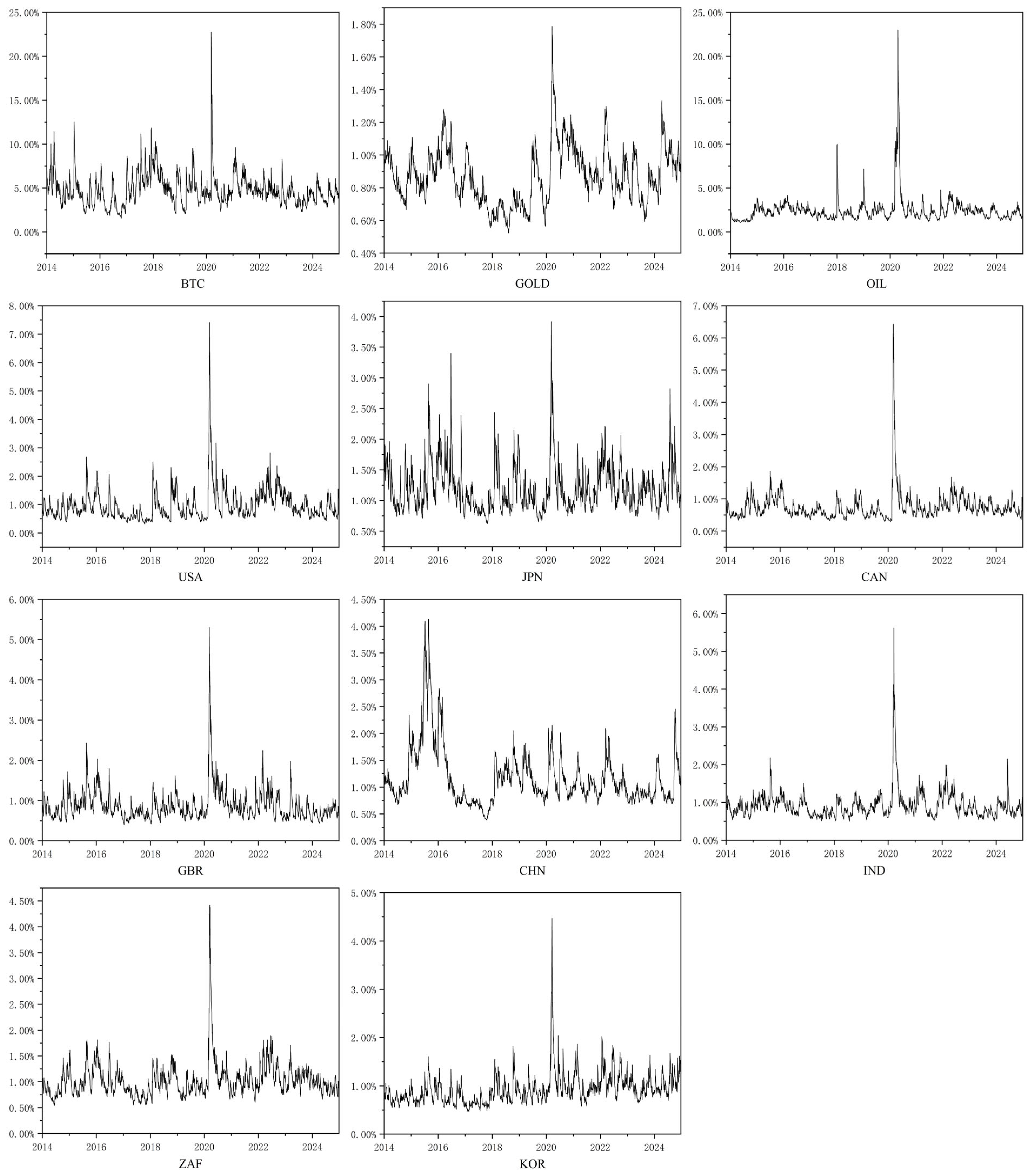
4.2.2. Conditional Volatility Dynamics

This study further conducts an in-depth analysis of the dynamic volatility of various assets based on the AR–EGARCH model. As shown in the volatility evolution in Figure 2 and the summary statistics in

Table 6. Descriptive statistics of the conditional volatility of the target assets.

	Categorization	Maximum	Minimum	Std.Dev	Mean	Rank
BTC	Cryptocurrency	22.7453%	1.5728%	1.8097%	4.7824%	1
GOLD	Commodity	1.7861%	0.5233%	0.1702%	0.8715%	10
OIL	Commodity	23.0062%	1.0559%	1.3909%	2.4076%	2
USA	Developed Market	7.4119%	0.3164%	0.5561%	0.9611%	6
JPN	Developed Market	3.9159%	0.6234%	0.3809%	1.2004%	3
CAN	Developed Market	6.4226%	0.2865%	0.4514%	0.7491%	11
GBR	Developed Market	5.3045%	0.3993%	0.3894%	0.8764%	9
CHN	Emerging Market	4.1333%	0.3899%	0.5400%	1.1765%	4
IND	Emerging Market	5.6214%	0.5020%	0.3732%	0.9191%	8
ZAF	Emerging Market	4.4153%	0.5431%	0.3416%	1.0230%	5
KOR	Emerging Market	4.4674%	0.4707%	0.3288%	0.9335%	7

, there are significant differences in both the temporal dynamics and magnitudes of volatility across asset classes. Bitcoin’s peak volatility reaches as high as 22.7453%, significantly exceeding that of all other asset classes. Moreover, the mean and standard deviation of its volatility are 4.7824% and 1.8097%, respectively, both the highest among the assets examined. These data reflect the exceptionally high and unstable volatility of Bitcoin. Crude oil ranks second in volatility, with a peak value of 23.0062% and a mean of 2.4076%. This elevated volatility may stem from the complex range of factors affecting commodity prices, including supply and demand shocks, as well as geopolitical risks. Both the oil and gold markets experienced sharp increases in volatility during the COVID-19 crisis. In contrast, gold has the lowest risk profile among all assets. Its maximum volatility is only 1.7861%, and although its mean value of 0.8715% is not the lowest, its standard deviation of just 0.1702% is significantly lower than that of other assets. The volatility path of gold is smoother, and its response to major events is notably weaker than that of equities or cryptocurrencies. These results confirm gold’s role as a safe-haven asset, particularly during periods of financial turmoil.

In the equity markets, the volatility gap between developed and emerging markets is relatively narrow. Among developed markets, Japan shows the highest average volatility at 1.2004%. The Japanese stock market experienced several brief surges in volatility between 2015 and 2016, primarily due to the Bank of Japan’s implementation of negative interest rates and ongoing quantitative easing policies. Volatility also rose significantly during the COVID-19 outbreak. The U.S. stock market exhibits a moderate average volatility of 0.9611%, with a notable spike only during the pandemic period. The U.K. and Canadian stock markets have the lowest volatility levels among equities, with mean values of 0.8764% and 0.7491%, respectively. Apart from the COVID-19 crisis, their volatility remained persistently low over time. Among emerging markets, China has the highest average volatility at 1.1765%. However, the volatility pattern of the Chinese stock market differs from other assets. During the COVID-19 pandemic, its volatility did not show a significant increase. Instead, the peak occurred during the 2015 Chinese stock market crisis. India, South Africa, and South Korea have average volatilities ranging from 0.91% to 1.03%, with standard deviations between 0.32% and 0.38%. These values indicate that while emerging markets overall face greater volatility pressure compared to developed markets, the differences are not as pronounced as those seen in the Bitcoin and oil markets. In these three emerging markets, the most evident volatility increases also occurred during the COVID-19 period. Overall, emerging markets exhibit higher volatility than most developed markets yet remain less volatile than crude oil and Bitcoin.

4.3. Tail Risk Analysis

Although volatility is widely used to measure the risk level of asset prices, it primarily reflects the magnitude of price fluctuations and is limited in its ability to directly quantify the maximum potential loss investors may face under extreme market conditions. To more effectively assess latent tail risks, this study incorporates the VaR framework to capture potential extreme losses. The analysis is conducted using a 95% confidence level, which is commonly adopted in the existing literature and has become one of the standard benchmarks for measuring tail risk.

4.3.1. Model Accuracy Evaluation and Comparative Analysis

This study develops two improved VaR forecasting models and compares them with traditional VaR approaches to evaluate their effectiveness in predicting tail risk. A key innovation in the model construction lies in the incorporation of skewed heavy-tailed distributions. The choice of distributional assumptions plays a critical role in enhancing the performance of GARCH-based models, as the accuracy of volatility estimation and VaR forecasts is highly sensitive to how well the return distribution is characterized.

Many scholars tend to assume that asset returns follow a normal distribution by default or apply a uniform heavy-tailed distribution without adequately considering the empirical features of the data, which may result in biased risk estimation (Deng et al. 2024). To address this issue, the GARCH models in this study incorporate not only the classical heavy-tailed distributions—such as the Student’s t-distribution (STD) and the generalized error distribution (GED)—but also their skewed counterparts, namely the skewed Student’s t-distribution (SSTD) and the skewed generalized error distribution (SGED), which capture both excess kurtosis and asymmetry. The AIC is employed to select the most appropriate distribution for each asset, with the aim of enhancing the accuracy of VaR predictions.

Table 7. AIC results of GARCH models for the target asset under different distributions.

	NORM	STD	GED	SSTD	SGED
BTC	−3.6264	−3.9284	−3.9241	−3.9275	−3.9233
GOLD	−6.6672	−6.7560	−6.7573	−6.7551	−6.7564
OIL	−4.7405	−4.8858	−4.8673	−4.8909	−4.8746
USA	−6.6509	−6.7486	−6.7351	−6.7588	−6.7463
JPN	−6.0782	−6.1344	−6.1351	−6.1358	−6.1378
CAN	−7.1256	−7.1652	−7.1544	−7.1920	−7.1860
GBR	−6.7799	−6.8333	−6.8252	−6.8472	−6.8421
CHN	−6.2323	−6.3379	−6.3330	−6.3385	−6.3348
IND	−6.6337	−6.7040	−6.6940	−6.7068	−6.6960
ZAF	−6.4100	−6.4371	−6.4331	−6.4427	−6.4391
KOR	−6.5994	−6.6323	−6.6333	−6.6377	−6.6394

reports the AIC values for the EGARCH model under different distributional assumptions. A lower AIC value indicates a better fit. The results show that Bitcoin, gold, and crude oil returns are best modeled with the STD, GED, and SSTD distributions, respectively. Among equity markets, the United States, Canada, the United Kingdom, China, India, and South Africa are best captured by the SSTD distribution, while the Japanese and South Korean stock markets are better suited to the SGED distribution.

Building on the distributional assumptions selected above, this study further integrates the VaR estimation process with a rolling window approach to dynamically assess risk levels through out-of-sample forecasting. At each time point, model parameters are estimated using only historical data within a fixed-size window, and the resulting estimates are then used to forecast the VaR for the next trading day. This approach effectively mitigates estimation bias caused by look-ahead information (Bali et al. 2008). By continuously discarding outdated observations and incorporating the most recent data, the rolling window mechanism reduces estimation noise associated with overly long sample periods and enhances the model’s responsiveness to sudden market shocks. In this study, the window size is set to 500 trading days to strike a balance between forecast accuracy and sample coverage (Alexander and Dakos 2023). The initial estimation window consists of the first 500 trading days prior to January 1, 2014. In addition to incorporating skewed heavy-tailed distributions and the rolling estimation procedure, this study further integrates the AR model, EGARCH model, and EVT to construct two improved VaR models: the AR–EGARCH–VaR model and the AR–EGARCH–EVT–VaR model. These hybrid models aim to enhance the predictive accuracy of tail risk forecasts across different asset classes.

This study first applies three traditional VaR estimation methods—historical simulation, Monte Carlo simulation, and GARCH–VaR—to systematically assess their predictive suitability under the current complex market conditions. On this basis, the AR–EGARCH model with normal distribution is introduced as a benchmark. The predictive accuracy of the two proposed VaR models is further evaluated using the Kupiec and Christoffersen tests and compared with traditional methods, enabling a systematic comparison of the forecasting performance of six VaR models across different asset classes under current market conditions.

Table 8. Results of the Kupiec test.

	Historical Simulation		Monte Carlo Simulation		GARCH
	LR	p-Value	LR	p-Value	LR	p-Value
BTC	1.1044	0.2933	3.5330	0.0602	1.3300	0.2488
GOLD	0.1966	0.6575	1.5775	0.2091	1.1044	0.2933
OIL	3.2016	0.0736	0.4155	0.5192	1.2648	0.2608
USA	0.1222	0.7267	0.0030	0.9566	6.4250	0.0113
JPN	0.2002	0.6546	0.0020	0.9645	1.2648	0.2608
CAN	0.0632	0.8015	0.9003	0.3427	6.9007	0.0086
GBR	0.4155	0.5192	2.4530	0.1173	3.2016	0.0736
CHN	0.8694	0.3511	0.9003	0.3427	0.1966	0.6575
IND	1.5775	0.2091	8.0676	0.0045	0.6988	0.4032
ZAF	0.1222	0.7267	0.4155	0.5192	7.3923	0.0066
KOR	0.0632	0.8015	0.4124	0.5207	2.8733	0.0901
	AR–EGARCH– Norm		AR–EGARCH		AR–EGARCH– EVT
	LR	p-Value	LR	p-Value	LR	p-Value
BTC	2.1388	0.1436	0.4124	0.5207	9.3533	0.0022
GOLD	0.2958	0.5866	0.2002	0.6546	0.5465	0.4598
OIL	0.2002	0.6546	1.0581	0.3036	1.4892	0.2223
USA	4.2873	0.0384	0.2002	0.6546	0.1222	0.7267
JPN	0.6988	0.4032	0.0207	0.8856	0.2002	0.6546
CAN	6.4250	0.0113	1.7312	0.1883	1.2648	0.2608
GBR	3.2016	0.0736	0.2970	0.5858	0.0632	0.8015
CHN	0.4155	0.5192	0.1222	0.7267	0.1966	0.6575
IND	0.1222	0.7267	0.1222	0.7267	0.1222	0.7267
ZAF	2.2678	0.1321	0.0632	0.8015	0.0030	0.9566
KOR	4.2873	0.0384	0.2970	0.5858	0.5465	0.4598

reports the results of the Kupiec test for each model at the 95% confidence level, which evaluates the unconditional coverage accuracy of VaR forecasts. According to the test criterion, a p-value greater than 0.1 indicates that the model does not significantly deviate from the theoretical violation rate, implying statistical adequacy. Higher p-values suggest a better alignment between the predicted VaR and the actual tail losses.

The results show that the historical simulation method fails to accurately estimate the VaR of the crude oil market, while the Monte Carlo simulation exhibits poor performance in forecasting the tail risk of Bitcoin and the Indian stock market. The GARCH–VaR model does not pass the test in several equity markets, suggesting its limited applicability under current volatile market conditions. Half of the stock markets fail the Kupiec test when VaR is estimated using the AR–EGARCH model with normal distribution. In contrast, the two improved models proposed in this study demonstrate superior overall performance. The AR–EGARCH–EVT–VaR model achieves high predictive accuracy for all assets except Bitcoin, whereas the AR–EGARCH–VaR model successfully passes the Kupiec test for all asset classes.

Table 9. Results of the Christoffersen test.

	Historical Simulation		Monte Carlo Simulation		GARCH
	LR	p-Value	LR	p-Value	LR	p-Value
BTC	5.3064	0.0704	11.8385	0.0027	4.1909	0.1230
GOLD	0.4334	0.8052	1.9920	0.3694	1.1967	0.5497
OIL	8.6433	0.0133	3.8110	0.1487	1.5823	0.4533
USA	19.8173	0.0000	18.4488	0.0001	7.2984	0.0260
JPN	12.0518	0.0024	11.4603	0.0032	11.1644	0.0038
CAN	29.4825	0.0000	28.1917	0.0000	16.4627	0.0003
GBR	14.0667	0.0009	12.1080	0.0023	5.9891	0.0501
CHN	8.7583	0.0125	10.8119	0.0045	1.9890	0.3699
IND	6.2205	0.0446	14.5114	0.0007	0.7115	0.7007
ZAF	1.0178	0.6012	0.4299	0.8066	7.4121	0.0246
KOR	32.8371	0.0000	37.1521	0.0000	10.2014	0.0061
	AR–EGARCH– Norm		AR–EGARCH		AR–EGARCH– EVT
	LR	p-Value	LR	p-Value	LR	p-Value
BTC	4.1394	0.1262	1.0552	0.5900	14.1648	0.0008
GOLD	1.2373	0.5387	0.4429	0.8014	1.1147	0.5727
OIL	0.2050	0.9026	2.0473	0.3593	2.2951	0.3174
USA	4.2965	0.1167	0.4429	0.8014	0.1355	0.9345
JPN	2.9202	0.2322	1.5061	0.4709	1.0506	0.5914
CAN	7.2984	0.0260	2.4529	0.2933	4.0731	0.1305
GBR	10.2453	0.0060	4.2236	0.1210	3.1884	0.2031
CHN	3.8110	0.1487	4.4689	0.1071	4.1909	0.1230
IND	1.8502	0.3965	1.8502	0.3965	1.8502	0.3965
ZAF	3.5212	0.1719	1.9890	0.3699	2.2159	0.3302
KOR	7.7161	0.0211	1.8325	0.4000	1.8480	0.3969

presents the results of the Christoffersen test. While the differences in VaR forecast accuracy among various models appear modest under the Kupiec test—with the exception of the GARCH–VaR model and AR–EGARCH model with normal distribution —traditional approaches such as the Monte Carlo simulation and historical simulation generally satisfy the unconditional coverage requirement. However, when time independence is taken into account via the Christoffersen test, these two methods fail in most asset categories, revealing significant weaknesses in capturing the temporal independence of VaR violations.

This shortcoming arises from the fundamental assumption underlying both historical and Monte Carlo simulations—that the distribution of future losses mirrors that of the past. As a result, these methods are unable to dynamically reflect volatility clustering. When markets experience consecutive episodes of high volatility, these models often fail to adjust the VaR threshold in a timely manner, leading to a temporal clustering of violations and, consequently, a failure to pass the Christoffersen test.

In contrast, the AR–EGARCH–VaR and AR–EGARCH–EVT–VaR models incorporate a conditional heteroskedastic structure that captures the asymmetric impact of past shocks. These models update the conditional volatility and corresponding VaR thresholds at each time point based on the most recent residual information. When market volatility intensifies, the models rapidly increase the VaR level, mitigating the clustering of violations; conversely, when volatility subsides, the VaR threshold is promptly reduced. This adaptive mechanism helps ensure that VaR exceedances are approximately independent over time, thus improving the likelihood of passing the Christoffersen conditional coverage test.

The test results indicate that none of the traditional methods are capable of reliably capturing the VaR of most assets under the current risk environment. By contrast, the AR–EGARCH–EVT–VaR model accurately captures the tail risk for all assets except Bitcoin. The AR–EGARCH–VaR model outperforms all others, successfully capturing the VaR dynamics for all target assets, thereby demonstrating superior robustness and broader applicability.

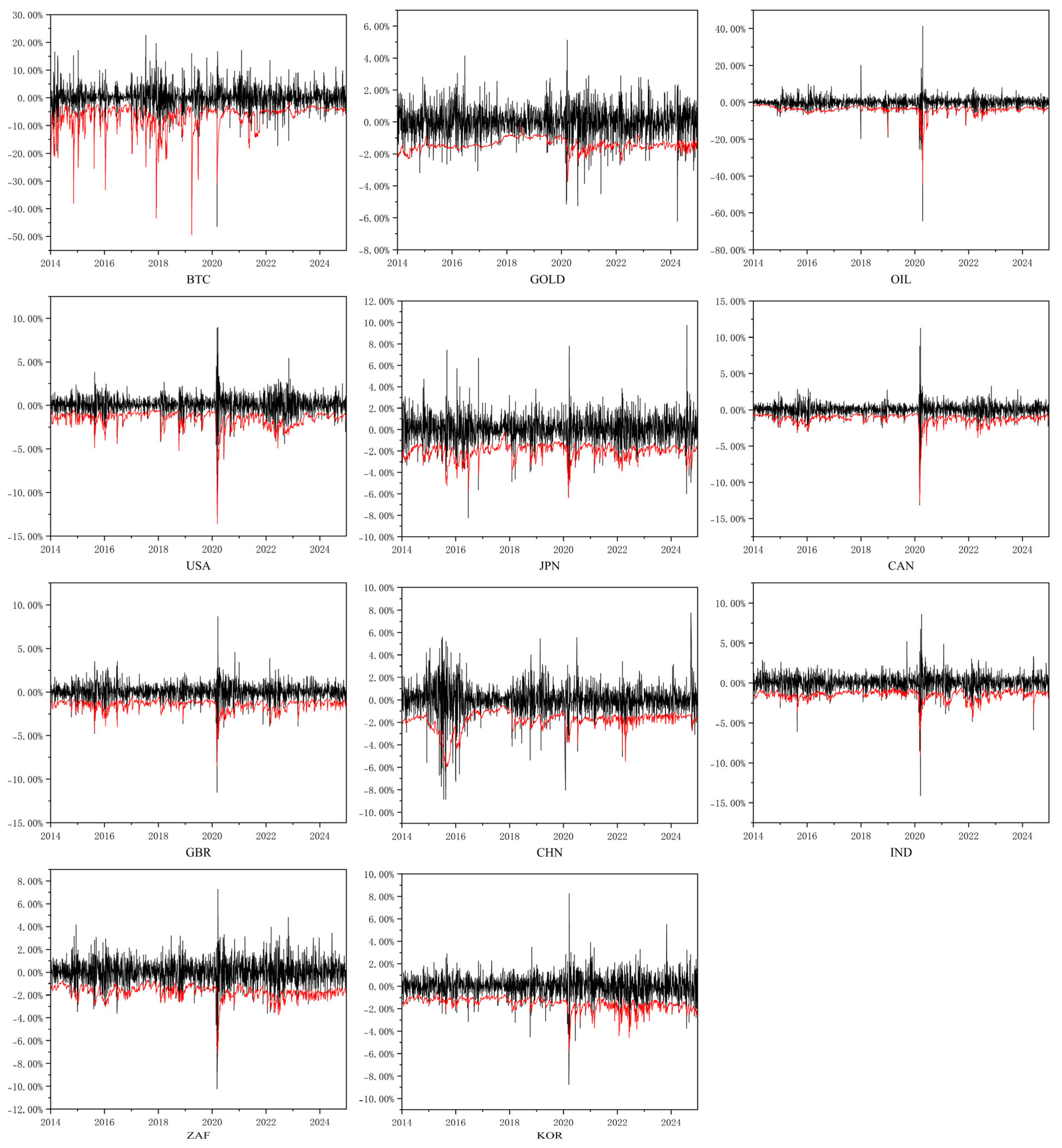
4.3.2. Comparative Analysis of Tail Risk

Since the VaR backtesting results confirm that the AR–EGARCH–VaR models incorporating skewed heavy-tailed distributions and rolling window estimation produce the most accurate VaR forecasts, this study further analyzes the mean and dynamic patterns of the 95% confidence level VaR estimates based on the AR–EGARCH–VaR. This analysis aims to compare the differences in tail risk across various asset classes. Figure 3 illustrates the time series of VaR values, where the black line represents the logarithmic returns and the red line indicates the corresponding VaR estimates.

Table 10. Descriptive statistics of the VaR of the target assets.

	Categorization	Whole Period	Rank	During Crisis	Rank
BTC	Cryptocurrency	−6.8829%	1	−6.7460%	1
GOLD	Commodity	−1.4310%	10	−1.6618%	11
OIL	Commodity	−3.8472%	2	−5.3084%	2
USA	Developed Market	−1.5682%	6	−2.2692%	3
JPN	Developed Market	−2.0273%	3	−2.0549%	4
CAN	Developed Market	−1.2630%	11	−1.7687%	10
GBR	Developed Market	−1.4998%	8	−2.0362%	6
CHN	Emerging Market	−1.8602%	4	−1.9867%	7
IND	Emerging Market	−1.4712%	9	−1.8876%	9
ZAF	Emerging Market	−1.7422%	5	−2.0577%	5

reports the average VaR values and rankings for the full sample period and for the COVID-19 crisis period. Given that VaR is inherently negative—its sign indicating direction rather than magnitude—this study focuses on the absolute values to assess risk levels.

In the whole period, Bitcoin exhibits the highest average VaR at 6.8829%, implying that investors face a 5% probability of incurring a daily loss exceeding this percentage. This value far exceeds that of other assets, highlighting the inherent leverage and speculative nature of the cryptocurrency market. Bitcoin’s high tail risk is largely attributable to its decentralized participant structure, widespread use of leverage, and lack of effective regulatory oversight, all of which make it highly sensitive to adverse news, such as regulatory crackdowns or exchange-related turmoil. Crude oil ranks second, with an average VaR of 3.8472%. As one of the world’s most important commodities, oil prices are subject to a broad range of influences—including production shocks, demand fluctuations, and geopolitical risks—which contribute to its elevated risk. In contrast, gold, a traditional safe-haven asset, has an average VaR of just 1.4310%, ranking second to last among all assets.

Among developed markets, Japan’s stock market has the highest average VaR at 2.0273%, which is consistent with its volatility ranking. This elevated level of risk may be linked to Japan’s long-standing structural economic stagnation. Despite its status as a developed economy, Japan has experienced prolonged low growth and persistent low or even negative interest rates. In addition, a loose exchange rate policy has facilitated cross-border capital flows, exacerbating tail risk in Japanese equities (Yoshino and Taghizadeh-Hesary 2016). In contrast, the U.S. and U.K. stock markets show moderate average VaR values of 1.5682% and 1.4998%, respectively. Canada’s stock market, with an average VaR of 1.2630%, has the lowest risk level among all assets, further underscoring its market stability. In emerging markets, China’s stock market exhibits the highest average VaR at 1.8602%, indicating that despite its global market capitalization ranking, China still faces structural challenges in regulatory effectiveness. Speculative behavior remains prevalent, contributing to elevated tail risk. South Africa, India, and South Korea show average VaR values ranging from 1.47% to 1.75%, generally higher than those of developed markets, reflecting the instability that often accompanies underdeveloped regulatory systems in emerging economies.

During the 2020 COVID-19 crisis, the daily VaR values of nearly all assets rose significantly, with noticeable differences across markets. Bitcoin’s average VaR declined slightly from 6.8892% to 6.7460%. Although still the highest in absolute terms, this slight reduction may reflect its growing role as a digital safe haven in the eyes of some investors during the pandemic (Mnif and Jarboui 2021). In contrast, crude oil’s average VaR surged from 3.8472% to 5.3084%, an increase of approximately 38%, making it one of the most severely affected assets. This dramatic rise reflects the sharp contraction in oil demand due to global lockdowns, which had a profound impact on prices.

Beyond cryptocurrencies and commodities, tail risks in developed stock markets also worsened during the crisis. The U.S. stock market’s average VaR rose from 1.5682% to 2.2692%, making it the riskiest equity market during COVID-19. This surge is largely attributable to the fact that the U.S. was one of the countries most severely affected by the pandemic, with approximately 50 million infections reported within the first eight months (Reese et al. 2021). The U.K. and Canadian markets also experienced increases, with average VaR values rising to 2.0362% and 1.7687%, respectively, underscoring the substantial impact of the pandemic on developed markets. Interestingly, Japan’s stock market saw only a modest increase in average VaR, from 2.0273% to 2.0549%—an increase of just 1%. This can be largely attributed to Japan’s early and effective containment of the pandemic without implementing widespread lockdowns. In emerging markets, China’s average VaR increased slightly from 1.8602% to 1.9867%, a rise of approximately 7%. This relatively moderate increase reflects the country’s highly effective pandemic response and public compliance, which helped contain extreme market risks (Yu and Li 2021). In contrast, other developing countries saw their average VaR rise by around 20%, revealing their vulnerability to external shocks. Although gold did not have the lowest average VaR during the full sample period, its increase during the COVID-19 crisis was minimal. In contrast, low-risk markets such as Canada experienced sharp increases in VaR. As a result, gold recorded the lowest average VaR of all assets during the crisis period, further confirming its role as a safe haven in times of extreme market stress.

5. Discussion

5.1. Research Conclusions

This study applies the AR–EGARCH model to examine the volatility characteristics of selected financial assets. The empirical results show that asset volatility is affected by both new information and past volatility, with the latter playing a more significant role. This suggests that financial markets exhibit strong memory, reflecting the lasting influence of investor sentiment and information flow on asset pricing. The model further reveals clear differences in volatility behavior across assets. The Chinese stock market and Bitcoin do not display significant asymmetric effects, meaning that their responses to positive and negative shocks are relatively balanced. This indicates that investor sentiment in these markets reacts similarly to good and bad news, suggesting stable market expectations. In contrast, gold exhibits a reverse leverage effect, where negative shocks lead to smaller increases in volatility compared to positive shocks. This implies that during periods of market stress, capital tends to move into gold, helping to limit its volatility. This supports gold’s traditional role as a safe-haven asset. Meanwhile, crude oil and the stock markets in the United States, Japan, Canada, the United Kingdom, India, South Africa, and South Korea show positive leverage effects, where negative shocks significantly increase volatility, indicating a higher sensitivity to adverse news.

In terms of average and dynamic volatility, Bitcoin and crude oil are the most volatile assets, reflecting both their speculative nature and strong reactions to external shocks. Gold, by contrast, shows the most stable volatility pattern, reinforcing its function as a store of value. Stock markets fall in between, with volatility levels that are moderate. Empirical evidence also suggests that emerging markets generally carry higher financial risk and volatility than developed markets. This pattern is widely supported by previous studies and is attributed to structural issues such as weaker financial systems, less efficient liquidity management, and more fragmented investor structures, all of which contribute to greater market instability (Harjoto and Rossi 2023; Uddin et al. 2021).

In terms of tail risk measurement, the results of the Kupiec and Christoffersen tests indicate that the three traditional VaR estimation methods—historical simulation, Monte Carlo simulation, and GARCH–VaR—are no longer suitable under current market conditions. In contrast, the two improved models developed in this study—the AR–EGARCH–VaR and AR–EGARCH–EVT–VaR models, both incorporating rolling window estimation and skewed heavy-tailed distributions—demonstrate significantly better predictive performance in estimating asset-specific VaR values. The comparison with the AR–EGARCH model under the normal distribution further confirms that the incorporation of fat-tailed distributions significantly improves the accuracy of VaR forecasts. Specifically, the AR–EGARCH–EVT–VaR model achieves relatively accurate VaR forecasts for most assets, with the exception of Bitcoin. The AR–EGARCH–VaR model, however, consistently performs well across all asset classes examined in this study, including both equity and non-equity assets, demonstrating strong cross-asset applicability. These findings offer investors and policymakers a more broadly applicable and statistically reliable VaR forecasting framework for accurately assessing the tail risks of diverse financial instruments.

Based on the AR–EGARCH–VaR model, which demonstrates the highest accuracy in VaR forecasting, this study further investigates the tail risk characteristics of the selected assets. The ranking of tail risk across assets is generally consistent with their volatility levels. During the COVID-19 crisis, most assets experienced a significant increase in tail risk, underscoring the destabilizing impact of global systemic events on financial markets. However, the increases in VaR for the Chinese and Japanese stock markets were relatively modest, potentially reflecting the effects of timely policy responses and effective macroeconomic interventions, suggesting that government actions remain crucial in mitigating systemic risk. Bitcoin also exhibited relatively stable tail risk during this period, indicating that its perceived role as a safe-haven asset may be gradually emerging despite ongoing debates. Gold maintained the lowest VaR level throughout the crisis, further reinforcing its function as a safe-haven asset under extreme market conditions. These findings highlight the heterogeneous nature of tail risk across different asset classes during major crises and provide important empirical evidence to guide investors in portfolio allocation and assist policymakers in designing effective risk regulation frameworks.

5.2. Policy Implications

From the perspective of investors, this study systematically reveals the volatility characteristics and tail risk profiles of various financial assets, offering quantitative support and theoretical guidance for portfolio allocation and risk management. Variations in assets’ leverage effects offer opportunities for portfolio diversification: investors may moderately increase their allocation to gold to exploit its inverse leverage effect as a hedge against volatility during market stress; maintain moderate to low positions in assets such as oil and major equity markets, which exhibit positive leverage effects, to limit downside risk; and include assets with relatively symmetric volatility responses, such as Bitcoin and the Chinese stock market, to enhance overall portfolio robustness. Based on the findings, investors should avoid blindly pursuing high-risk assets. Instead, investment decisions should be made in accordance with individual risk tolerance and preferences. Risk-seeking investors may consider allocating a portion of their portfolios to high-volatility assets such as crude oil, Bitcoin, and Japanese equities in pursuit of higher returns. In contrast, risk-averse investors are advised to focus on assets with relatively stable risk profiles, such as gold and equities from developed markets, by reducing exposure to high-risk positions to achieve better diversification and wealth preservation. Investors are encouraged to fully utilize the AR–EGARCH–VaR model developed and validated in this study to dynamically monitor changes in tail risk and adjust portfolio structures in a timely manner. Doing so will enable more effective control of potential losses under extreme market conditions.

In addition, the empirical results show that the tail risk levels of all asset classes increased significantly during the COVID-19 pandemic, highlighting the widespread and profound impact of systemic crises on financial stability. In light of this, investors should enhance their risk awareness when facing similar future crises. Specifically, in the early stages of a crisis, reducing exposure may help avoid extreme losses driven by market shocks. In the later stages, however, panic-driven sell-offs are often irrational. During such periods, investors may consider reallocating toward fundamentally sound and resilient assets—such as high-quality equities or gold—as a means of preserving value while awaiting a recovery in market sentiment and normalization of risk levels.

For policymakers, the AR–EGARCH–VaR model proposed in this study can serve as an effective tool for monitoring and forecasting market risk. It enables regulators to dynamically assess tail risk across major financial assets and adjust macroprudential and regulatory policies accordingly. Policymakers should recognize the substantial heterogeneity in risk levels across asset classes. Especially during global crises or periods of heightened market volatility, regulatory responses should be tailored to the specific risk characteristics of different asset types. Uniform policy measures applied across highly dissimilar assets may weaken regulatory effectiveness. For high-risk assets, regulatory authorities may consider setting limits on portfolio exposure and increasing capital buffer requirements to enhance the resilience of financial institutions against large price fluctuations. In addition, institutions can be required to regularly report their risk exposures and projected losses, enabling dynamic monitoring of potential tail risks. In contrast, for low-risk assets with relatively low volatility, exposure limits may be relaxed, and such assets can be allowed to serve as liquidity support instruments during periods of market stress. By implementing a differentiated regulatory approach—combining “exposure constraints and capital buffers” for high-risk assets with “allocation incentives and liquidity support” for low-risk assets—regulators can help mitigate the buildup of systemic risk while improving the stability and efficiency of the financial system.

Furthermore, since emerging markets typically face higher risk exposures compared to developed markets, policymakers in these economies should acknowledge the structural gaps and work toward improving regulatory frameworks and market governance. Strengthening domestic financial resilience and long-term market stability will require a more robust institutional infrastructure. At the policy level, it is recommended that priority be given to improving and standardizing the regulatory framework, with a focus on enhancing financial institutions’ capacity for risk identification and capital management. In parallel, efforts should be made to strengthen market governance by increasing the transparency of information disclosure and reinforcing oversight of market conduct in order to reduce information asymmetry and systemic vulnerabilities. Building on this foundation, emerging markets should gradually establish a macroprudential framework tailored to their domestic risk characteristics, such as introducing countercyclical capital buffers and developing systems to monitor cross-market risk linkages. These measures would help enhance the overall resilience and stability of the financial system, thereby improving the capacity to withstand external shocks. In addition, the establishment of a sound risk disclosure mechanism can help convey timely and transparent warnings to the market, reduce information asymmetry, and mitigate irrational investment behavior and systemic panic. Such measures are essential for maintaining the long-term health and stability of the financial system.

References

1. Afzal, Fahim, Pan Haiying, Farman Afzal, Asif Mahmood, and Amir Ikram. 2021. Value-at-risk analysis for measuring stochastic volatility of stock returns: Using GARCH-based dynamic conditional correlation model. Sage Open 11: 21582440211005758. [Google Scholar] [CrossRef]
2. Alexander, Carol, and Michael Dakos. 2023. Assessing the accuracy of exponentially weighted moving average models for Value-at-Risk and Expected Shortfall of crypto portfolios. Quantitative Finance 23: 393–427. [Google Scholar] [CrossRef]
3. Bali, Turan G., Hengyong Mo, and Yi Tang. 2008. The role of autoregressive conditional skewness and kurtosis in the estimation of conditional VaR. Journal of Banking & Finance 32: 269–82. [Google Scholar] [CrossRef]
4. Banihashemi, Shokoofeh, and Sarah Navidi. 2017. Portfolio performance evaluation in Mean-CVaR framework: A comparison with non-parametric methods value at risk in Mean-VaR analysis. Operations Research Perspectives 4: 21–28. [Google Scholar] [CrossRef]
5. Batten, Jonathan A., Harald Kinateder, and Peter G. Szilagyi. 2024. Should you buy gold stocks or paper gold? Finance Research Letters 69: 106202. [Google Scholar] [CrossRef]
6. Baur, Dirk G., and Allan Trench. 2022. Not all gold shines in crisis times—Gold firms, gold bullion and the COVID-19 shock. Journal of Commodity Markets 28: 100260. [Google Scholar] [CrossRef]
7. Baur, Dirk G., Lai T. Hoang, and Md Zakir Hossain. 2022. Is Bitcoin a hedge? How extreme volatility can destroy the hedge property. Finance Research Letters 47: 102655. [Google Scholar] [CrossRef]
8. Bekaert, Geert, Campbell R. Harvey, and Tomas Mondino. 2023. Emerging equity markets in a globalized world. Emerging Markets Review 56: 101034. [Google Scholar] [CrossRef]
9. Blau, Benjamin M., Todd G. Griffith, and Ryan J. Whitby. 2021. Inflation and Bitcoin: A descriptive time-series analysis. Economics Letters 203: 109848. [Google Scholar] [CrossRef]
10. Bollerslev, Tim. 1986. Generalized autoregressive conditional heteroskedasticity. Journal of Econometrics 31: 307–27. [Google Scholar] [CrossRef]
11. Boonman, Tjeerd M. 2023. Portfolio capital flows before and after the Global Financial Crisis. Economic Modelling 127: 106440. [Google Scholar] [CrossRef]
12. Boubaker, Heni, Juncal Cunado, Luis A. Gil-Alana, and Rangan Gupta. 2020. Global crises and gold as a safe haven: Evidence from over seven and a half centuries of data. Physica A: Statistical Mechanics and Its Applications 540: 123093. [Google Scholar] [CrossRef]
13. Chincarini, Ludwig B., and Fabio Moneta. 2021. The challenges of oil investing: Contango and the financialization of commodities. Energy Economics 102: 105443. [Google Scholar] [CrossRef]
14. Christoffersen, Peter F. 1998. Evaluating interval forecasts. International Economic Review 39: 841–62. [Google Scholar] [CrossRef]
15. Das, Nupur Moni, Bhabani Sankar Rout, and Yashmin Khatun. 2023. Does G7 engross the shock of COVID 19: An assessment with market volatility? Asia-Pacific Financial Markets 30: 795–816. [Google Scholar] [CrossRef]
16. Deng, Xue, Wen Zhou, Fengting Geng, and Yuan Lu. 2024. A novel ARMA-GARCH-Sent-EVT-Copula Portfolio model with investor sentiment. Soft Computing 28: 13501–26. [Google Scholar] [CrossRef]
17. Díaz, Antonio, Carlos Esparcia, and Raquel López. 2022. The diversifying role of socially responsible investments during the COVID-19 crisis: A risk management and portfolio performance analysis. Economic Analysis and Policy 75: 39–60. [Google Scholar] [CrossRef] [PubMed]
18. Echaust, Krzysztof, and Małgorzata Just. 2020. Value at risk estimation using the GARCH-EVT approach with optimal tail selection. Mathematics 8: 114. [Google Scholar] [CrossRef]
19. Fiszeder, Piotr, Marta Małecka, and Peter Molnár. 2024. Robust estimation of the range-based GARCH model: Forecasting volatility, value at risk and expected shortfall of cryptocurrencies. Economic Modelling 141: 106887. [Google Scholar] [CrossRef]
20. Gomis-Porqueras, Pedro, Shuping Shi, and David Tan. 2022. Gold as a financial instrument. Journal of Commodity Markets 27: 100218. [Google Scholar] [CrossRef]
21. Grout, Paul A., and Anna Zalewska. 2016. Stock market risk in the financial crisis. International Review of Financial Analysis 46: 326–45. [Google Scholar] [CrossRef]
22. Halkos, George E., and Apostolos S. Tsirivis. 2019. Value-at-risk methodologies for effective energy portfolio risk management. Economic Analysis and Policy 62: 197–212. [Google Scholar] [CrossRef]
23. Harjoto, Maretno Agus, and Fabrizio Rossi. 2023. Market reaction to the COVID-19 pandemic: Evidence from emerging markets. International Journal of Emerging Markets 18: 173–99. [Google Scholar] [CrossRef]
24. He, Dong. 2021. Digitalization of cross-border payments. China Economic Journal 14: 26–38. [Google Scholar] [CrossRef]
25. Hodoshima, Jiro, and Nana Otsuki. 2019. Evaluation by the Aumann and Serrano performance index and Sharpe ratio: Bitcoin performance. Applied Economics 51: 4282–98. [Google Scholar] [CrossRef]
26. Hong, Hui, Zhicun Bian, and Chien-Chiang Lee. 2021. COVID-19 and instability of stock market performance: Evidence from the US. Financial Innovation 7: 1–18. [Google Scholar] [CrossRef] [PubMed]
27. Huang, Yongrong, Huiqing Wang, Zhide Chen, Chen Feng, Kexin Zhu, Xu Yang, and Wencheng Yang. 2024. Evaluating cryptocurrency market risk on the blockchain: An empirical study using the ARMA-GARCH-VaR model. IEEE Open Journal of the Computer Society 5: 83–94. [Google Scholar] [CrossRef]
28. Irfan, Muhammad, Mubeen Abdur Rehman, Sarah Nawazish, and Yu Hao. 2023. Performance analysis of gold-and fiat-backed cryptocurrencies: Risk-based choice for a portfolio. Journal of Risk and Financial Management 16: 99. [Google Scholar] [CrossRef]
29. Izzeldin, Marwan, Yaz Gülnur Muradoğlu, Vasileios Pappas, and Sheeja Sivaprasad. 2021. The impact of COVID-19 on G7 stock markets volatility: Evidence from a ST-HAR model. International Review of Financial Analysis 74: 101671. [Google Scholar] [CrossRef] [PubMed]
30. Kang, Wenjin, Ke Tang, and Ningli Wang. 2023. Financialization of commodity markets ten years later. Journal of Commodity Markets 30: 100313. [Google Scholar] [CrossRef]
31. Kim, Jong-Min, Dong H. Kim, and Hojin Jung. 2021. Estimating yield spreads volatility using GARCH-type models. The North American Journal of Economics and Finance 57: 101396. [Google Scholar] [CrossRef]
32. Koulis, Alexandros, and Constantinos Kyriakopoulos. 2023. On volatility transmission between gold and silver markets: Evidence from a long-term historical period. Computation 11: 25. [Google Scholar] [CrossRef]
33. Krause, David. 2024. Mainstreaming Cryptocurrency: The State of Wisconsin Investment Board’s Pioneering Investment in Bitcoin ETFs. Available online: https://papers.ssrn.com/sol3/papers.cfm?abstract_id=4852566 (accessed on 10 July 2025).
34. Kupabado, Moses Mananyi, and Juergen Kaehler. 2025. Price effects of commodity financialization: Review of the evidence. Journal of Economic Surveys 39: 352–74. [Google Scholar] [CrossRef]
35. Kupiec, Paul H. 1995. Techniques for Verifying the Accuracy of Risk Measurement Models. Washington, DC: Division of Research and Statistics, Division of Monetary Affairs, Federal Reserve Board,, vol. 95. [Google Scholar]
36. Li, Yang, and Qingfeng Du. 2024. Oil price volatility and gold prices volatility asymmetric links with natural resources via financial market fluctuations: Implications for green recovery. Resources Policy 88: 104279. [Google Scholar] [CrossRef]
37. Likitratcharoen, Danai, and Lucksuda Suwannamalik. 2024. Assessing Financial Stability in Turbulent Times: A Study of Generalized Autoregressive Conditional Heteroskedasticity-Type Value-at-Risk Model Performance in Thailand’s Transportation Sector during COVID-19. Risks 12: 51. [Google Scholar] [CrossRef]
38. Likitratcharoen, Danai, Pan Chudasring, Chakrin Pinmanee, and Karawan Wiwattanalamphong. 2023. The efficiency of value-at-risk models during extreme market stress in cryptocurrencies. Sustainability 15: 4395. [Google Scholar] [CrossRef]
39. Lin, Zhe. 2018. Modelling and forecasting the stock market volatility of SSE Composite Index using GARCH models. Future Generation Computer Systems 79: 960–72. [Google Scholar] [CrossRef]
40. Lyu, Yongjian, Siwei Tuo, Yu Wei, and Mo Yang. 2021. Time-varying effects of global economic policy uncertainty shocks on crude oil price volatility: New evidence. Resources Policy 70: 101943. [Google Scholar] [CrossRef]
41. Mazur, Mieszko, Man Dang, and Miguel Vega. 2021. COVID-19 and the march 2020 stock market crash. Evidence from S&P1500. Finance Research Letters 38: 101690. [Google Scholar] [CrossRef] [PubMed]
42. Mnif, Emna, and Anis Jarboui. 2021. COVID-19, bitcoin market efficiency, herd behaviour. Review of Behavioral Finance 13: 69–84. [Google Scholar] [CrossRef]
43. Mrkvička, Tomáš, Martina Krásnická, Ludvík Friebel, Tomáš Volek, and Ladislav Rolínek. 2022. Backtesting the evaluation of Value-at-Risk methods for exchange rates. Studies in Economics and Finance 40: 175–91. [Google Scholar] [CrossRef]
44. Nelson, Daniel B. 1991. Conditional heteroskedasticity in asset returns: A new approach. Econometrica: Journal of the Econometric Society 59: 347–70. [Google Scholar] [CrossRef]
45. Nguyen, Quang Thi Thieu, Dao Le Trang Anh, and Christopher Gan. 2021. Epidemics and Chinese firms’ stock returns: Is COVID-19 different? China Finance Review International 11: 302–21. [Google Scholar] [CrossRef]
46. Pan, Zhiyuan, Xiao Huang, Li Liu, and Juan Huang. 2023. Geopolitical uncertainty and crude oil volatility: Evidence from oil-importing and oil-exporting countries. Finance Research Letters 52: 103565. [Google Scholar] [CrossRef]
47. Patra, Saswat. 2021. Revisiting value-at-risk and expected shortfall in oil markets under structural breaks: The role of fat-tailed distributions. Energy Economics 101: 105452. [Google Scholar] [CrossRef]
48. Patra, Saswat, and Neha Gupta. 2023. Risk in the cryptocurrency markets: The role of structural breaks and fat-tailed distributions in estimating value-at-risk and expected shortfall. The European Journal of Finance, 1–21. [Google Scholar] [CrossRef]
49. Raggad, Bechir, and Elie Bouri. 2023. Gold and crude oil: A time-varying causality across various market conditions. Resources Policy 86: 104273. [Google Scholar] [CrossRef]
50. Rahman, Md Lutfur, Abu Amin, and Mohammed Abdullah Al Mamun. 2021. The COVID-19 outbreak and stock market reactions: Evidence from Australia. Finance Research Letters 38: 101832. [Google Scholar] [CrossRef] [PubMed]
51. Ranković, Vladimir, Mikica Drenovak, Branko Urosevic, and Ranko Jelic. 2016. Mean-univariate GARCH VaR portfolio optimization: Actual portfolio approach. Computers & Operations Research 72: 83–92. [Google Scholar]
52. Reese, Heather, A. Danielle Iuliano, Neha N. Patel, Shikha Garg, Lindsay Kim, Benjamin J. Silk, Aron J. Hall, Alicia Fry, and Carrie Reed. 2021. Estimated incidence of coronavirus disease 2019 (COVID-19) illness and hospitalization—United States, February–September 2020. Clinical Infectious Diseases 72: e1010–e1017. [Google Scholar] [CrossRef] [PubMed]
53. Ren, Xiaohang, Ya Xiao, Feng He, and Giray Gozgor. 2024. The contagion of extreme risks between fossil and green energy markets: Evidence from China. Quantitative Finance 24: 627–42. [Google Scholar] [CrossRef]
54. Rout, Bhabani Sankar, Nupur Moni Das, and Mohd Merajuddin Inamdar. 2021. COVID-19 and market risk: An assessment of the G-20 nations. Journal of Public Affairs 21: e2590. [Google Scholar] [CrossRef] [PubMed]
55. Salisu, Afees A., Ibrahim D. Raheem, and Xuan Vinh Vo. 2021. Assessing the safe haven property of the gold market during COVID-19 pandemic. International Review of Financial Analysis 74: 101666. [Google Scholar] [CrossRef] [PubMed]
56. Setiawan, Budi, Marwa Ben Abdallah, Maria Fekete-Farkas, Robert Jeyakumar Nathan, and Zoltan Zeman. 2021. GARCH (1, 1) models and analysis of stock market turmoil during COVID-19 outbreak in an emerging and developed economy. Journal of Risk and Financial Management 14: 576. [Google Scholar] [CrossRef]
57. Soleymani, Fazlollah, Qiang Ma, and Tao Liu. 2025. Managing the risk via the Chi-squared distribution in VaR and CVaR with the use in generalized autoregressive conditional heteroskedasticity model. Mathematics 13: 1410. [Google Scholar] [CrossRef]
58. Su, Chi-Wei, Lidong Pang, Muhammad Umar, and Oana-Ramona Lobonţ. 2022. Will gold always shine amid world uncertainty? Emerging Markets Finance and Trade 58: 3425–38. [Google Scholar] [CrossRef]
59. Tanin, Tauhidul Islam, Ashutosh Sarker, Robert Brooks, and Hung Xuan Do. 2022. Does oil impact gold during COVID-19 and three other recent crises? Energy Economics 108: 105938. [Google Scholar] [CrossRef] [PubMed]
60. Triki, Mohamed Bilel, and Abderrazek Ben Maatoug. 2021. The GOLD market as a safe haven against the stock market uncertainty: Evidence from geopolitical risk. Resources Policy 70: 101872. [Google Scholar] [CrossRef]
61. Uddin, Moshfique, Anup Chowdhury, Keith Anderson, and Kausik Chaudhuri. 2021. The effect of COVID–19 pandemic on global stock market volatility: Can economic strength help to manage the uncertainty? Journal of Business Research 128: 31. [Google Scholar] [CrossRef] [PubMed]
62. Usman, Abdullahi Ubale, Sunusi Bala Abdullahi, Yu Liping, Bayan Alghofaily, Ahmed S. Almasoud, and Amjad Rehman. 2024. Financial Fraud Detection Using Value-at-Risk with Machine Learning in Skewed Data. IEEE Access 12: 64285–99. [Google Scholar] [CrossRef]
63. Wang, Weibin, and Yao Wu. 2023. Risk analysis of the Chinese financial market with the application of a novel hybrid volatility prediction model. Mathematics 11: 3937. [Google Scholar] [CrossRef]
64. Wang, Xinya, Brian Lucey, and Shupei Huang. 2022. Can gold hedge against oil price movements: Evidence from GARCH-EVT wavelet modeling. Journal of Commodity Markets 27: 100226. [Google Scholar] [CrossRef]
65. Xu, Yingying, and Donald Lien. 2022. Forecasting volatilities of oil and gas assets: A comparison of GAS, GARCH, and EGARCH models. Journal of Forecasting 41: 259–78. [Google Scholar] [CrossRef]
66. Yang, Jing Yu, Minyoung Kim, Jiatao Li, and Jane Wenzhen Lu. 2023. Information voids and cross-border bandwagons of foreign direct investment into an emerging economy. Strategic Management Journal 44: 2751–82. [Google Scholar] [CrossRef]
67. Yen-Ku, Kuo, Apichit Maneengam, Phan The Cong, Nguyen Ngoc Quynh, Mohammed Moosa Ageli, and Worakamol Wisetsri. 2022. COVID-19 and oil and gold price volatilities: Evidence from China market. Resources Policy 79: 103024. [Google Scholar] [CrossRef] [PubMed]
68. Yoshino, Naoyuki, and Farhad Taghizadeh-Hesary. 2016. Causes and remedies of the Japan’s long-lasting recession: Lessons for China. China & World Economy 24: 23–47. [Google Scholar]
69. Yu, Xiang, and Na Li. 2021. Understanding the beginning of a pandemic: China’s response to the emergence of COVID-19. Journal of Infection and Public Health 14: 347–52. [Google Scholar] [CrossRef] [PubMed]
70. Yu, Yang, SongLin Guo, and XiaoChen Chang. 2022. Oil prices volatility and economic performance during COVID-19 and financial crises of 2007–2008. Resources Policy 75: 102531. [Google Scholar] [CrossRef] [PubMed]
71. Zhang, Chen, and Xinmiao Zhou. 2024. Forecasting value-at-risk of crude oil futures using a hybrid ARIMA-SVR-POT model. Heliyon 10: e23358. [Google Scholar] [CrossRef] [PubMed]
72. Zhang, Chun-Xia, Jun Li, Xing-Fang Huang, Jiang-She Zhang, and Hua-Chuan Huang. 2022. Forecasting stock volatility and value-at-risk based on temporal convolutional networks. Expert Systems with Applications 207: 117951. [Google Scholar] [CrossRef]
73. Zhang, Weiping, Xintian Zhuang, and Yang Lu. 2020. Spatial spillover effects and risk contagion around G20 stock markets based on volatility network. The North American Journal of Economics and Finance 51: 101064. [Google Scholar] [CrossRef]
74. Zhang, Wenwen, Shuo Cao, Xuan Zhang, and Xuefeng Qu. 2023. COVID-19 and stock market performance: Evidence from the RCEP countries. International Review of Economics & Finance 83: 717–35. [Google Scholar]
Figure 1. Logarithmic return of the target assets.
Risks 13 00138 g001
Figure 2. The conditional volatility of the target assets.
Risks 13 00138 g002
Figure 3. The VaR of the target assets.
Risks 13 00138 g003