Identifying Risk Regimes in a Sectoral Stock Index Through a Multivariate Hidden Markov Framework

Abstract

This study explores the presence of hidden market regimes in a sector-specific stock index within the Thai equity market. The behavior of such indices often deviates from broader macroeconomic trends, making it difficult for conventional models to detect regime changes. To overcome this limitation, the study employs a multivariate Gaussian mixture hidden Markov model, which enables the identification of unobservable states based on daily and intraday return patterns. These patterns include open-to-close, open-to-high, and low-to-open returns. The model is estimated using various specifications, and the best-performing structure is chosen based on the Akaike Information Criterion and the Bayesian Information Criterion. The final model reveals three statistically distinct regimes that correspond to bullish, sideways, and bearish conditions. Statistical tests, particularly the Kruskal–Wallis method, confirm that return distributions, trading volume, and open interest differ significantly across these regimes. Additionally, the analysis incorporates risk measures, including expected shortfall, maximum drawdown, and the coefficient of variation. The results indicate that the bearish regime carries the highest risk, whereas the bullish regime is relatively stable. These findings offer practical insights for regime-aware portfolio management in sectoral equity markets.

1. Introduction

Sector-specific equity indices often exhibit dynamics that differ from broader market benchmarks and macroeconomic trends. Their price behavior may reflect localized structural shifts, sentiment cycles, and supply-side conditions that are not always observable through standard economic indicators. These latent shifts contribute to the emergence of distinct market regimes, the periods during which return distributions, volatility levels, and liquidity patterns follow different statistical behaviors. Identifying such regimes promptly is crucial for investors seeking to enhance portfolio resilience and risk-adjusted performance (Dzwigol et al. 2021).

Economic factors affecting logistics activities influence the return on investment, although these factors may not have an immediate impact. This results in the market regime, or investment conditions in industry-level equity stocks, not necessarily aligning directly with economic cycles. Furthermore, market regimes, such as bullish or bearish markets, also affect investor psychology in different ways (Andrew and Timmermann 2012). Changes in market structures driven by economic conditions may alter the relationship between specific features and the returns on sectoral stock assets.

Traditional models used for regime detection, such as Autoregressive Integrated Moving Average (ARIMA) or Generalized Autoregressive Conditional Heteroskedasticity (GARCH) frameworks, generally assume static relationships among variables and often rely on explicit economic inputs. While effective in some settings, these models are limited in their ability to adapt to changing market structures, especially when the drivers of change are unobservable or time-varying. Additionally, supervised learning models tend to underperform when latent state transitions are not well-aligned with predefined labels or economic conditions. (Nguyen et al. 2018).

In contrast, hidden Markov models (HMMs) offer a probabilistic and unsupervised framework for modeling stochastic transitions between latent states. The extended Gaussian mixture hidden Markov model (gmHMM) accommodates multivariate, non-Gaussian distributions of returns, making it well-suited for modeling the complexities of sectoral stock dynamics. Despite its increasing application in macro-financial contexts, the integration of this approach into sector-focused modeling remains underexplored. Prior studies have applied gmHMMs in the context of equity forecasting and trading strategy design (Kijkarncharoensin and Maneerat 2024; Kijkarncharoensin, forthcoming), yet applications at the sectoral index level remain limited.

This study applies a multivariate gmHMM—a framework that combines hidden state modeling with Gaussian mixture emissions—to a sectoral stock index in an emerging market. The model captures three types of daily returns—open-to-close, open-to-high, and low-to-open—as observable signals. The primary objectives are threefold: (1) to empirically identify the number of latent risk regimes, (2) to characterize each regime in terms of return distributions and downside risks, and (3) to interpret their practical implications for regime-aware investment decisions. The modeling framework also provides a foundation for assessing the expected shortfall, maximum drawdown, and the coefficient of variation across different regimes, enabling a more enriched understanding of sector-specific market risk.

By offering a replicable and interpretable framework grounded in the gmHMM, this research aims to contribute to both financial econometrics and applied investment strategy. Its relevance extends to practitioners and policymakers seeking early-warning indicators of regime transitions within volatile sectors. The findings are also expected to inform future enhancements in data-driven regime classification models in emerging equity markets.

The remainder of this paper is structured as follows. Section 2 provides a review of the relevant literature, establishing the conceptual foundation for the current study. Section 3 outlines the theoretical and methodological framework, with a particular focus on the structure and estimation of the Gaussian mixture hidden Markov model. Section 4 reports the empirical results, followed by Section 5, which offers a discussion of the main findings and their practical implications. Section 6 presents the data, variable construction, and research design. Finally, Section 7 concludes the paper and suggests potential avenues for future research.

2. Literature Review

Research on regime-switching behavior in financial markets has been enriched by the application of hidden Markov models (HMMs), particularly the Gaussian mixture variant (gmHMM), which provides a robust statistical framework for capturing unobservable states that influence observable asset dynamics. This modeling approach traces its theoretical origins to foundational works by Baum and Eagon (1967), Levinson et al. (1983), and Liporace (1982), who formalized the probabilistic mechanisms underlying latent state transitions and continuous-valued emissions. These advances were later extended by Juang (1985), Juang et al. (1986), Gauvain and Lee (1994), and Li et al. (2000) to accommodate multivariate Gaussian mixtures, significantly broadening the applicability of HMMs to financial time series, where market behavior often deviates from normality and symmetry.

In the context of financial applications, Rabiner’s (1989) expository work laid the groundwork for adapting HMMs beyond engineering to market data. Hassan and Nath (2005) demonstrated the effectiveness of gmHMMs in forecasting stock movements using OHLC prices, while Gupta and Dhingra (2012) emphasized the use of return-based emissions, showing the model’s flexibility in capturing return volatility. Nguyen (2017, 2018) further advanced the framework by integrating model selection criteria, such as the Akaike Information Criterion (AIC) and the Bayesian Information Criterion (BIC), for parameter estimation and employing the Viterbi path to optimize trading signal generation. These studies illustrate the evolution of HMMs from their algorithmic roots to practical investment strategies and asset allocation decisions under regime uncertainty.

Recent literature has emphasized the broader economic interpretations of latent states identified by gmHMMs. Manjunatha et al. (2024) provide a rigorous foundation for applying gmHMMs to financial systems, detailing the mathematical structure of emission probabilities and their relation to systemic risk detection. Their synthesis positions gmHMM as a powerful lens through which asset return dynamics, shaped by structural economic shifts, can be systematically decoded. Similarly, Neal et al. (2024) advance the discussion by proposing a multivariate HMM for panel data, extending traditional HMMs to capture heterogeneous regime responses across firms or sectors. This development enhances the ability to model cross-sectional dependence, which is essential in sectoral studies where co-movements are pronounced.

The integration of machine learning with latent variable models has garnered increasing attention. Sivakumar (2025) proposes an HMM–LSTM fusion architecture that captures temporal dependencies in macroeconomic time series, resulting in improved forecasting accuracy compared to traditional HMMs. In parallel, Catello et al. (2023) validated the predictive capacity of HMMs in stock market classification by coupling them with supervised learning models, such as decision trees and neural networks, underscoring the practical synergy between probabilistic regime inference and discriminative classification techniques. This approach parallels earlier efforts in applying unsupervised learning to domain-specific data clustering, such as biomass classification using thermal properties (Kijkarncharoensin and Innet 2022, 2023a, 2023b), thereby reinforcing the general utility of latent-pattern discovery across fields where structural labeling is impractical.

Additionally, the literature has begun to focus on the role of latent regimes in explaining volatility clustering and macroeconomic fluctuations. Lenart et al. (2024) introduced a Bayesian nonlinear stationary model with multiple frequencies, revealing that regimes often correspond to distinct cyclical patterns not observable through conventional time-series decomposition. In a related contribution, Jahan-Parvar et al. (2024) presented a Bayesian multivariate unobserved components model, which allows for the concurrent estimation of trend-cycle dynamics and regime effects across multiple financial variables. These studies support the theoretical claim that regime identification is not merely a statistical convenience but a necessary component of understanding the structural transformations in economic behavior.

Despite this substantial progress, existing literature has predominantly focused on aggregate market indices, macroeconomic variables, or global equity benchmarks, leaving a relative gap in the application of gmHMMs to sector-specific indices in emerging markets. While Kijkarncharoensin and Maneerat (2024) and Kijkarncharoensin (forthcoming) applied gmHMMs in general equity contexts, the unique volatility structure and cyclical behavior of individual sectors remain underexplored. This omission is critical because sectoral indices often exhibit distinct sensitivity to economic policies, supply chain dynamics, and global trade disruptions, making them fertile ground for identifying nuanced regime behavior.

The present study addresses this research gap by applying a multivariate gmHMM to the Thai Logistics Sector Index (TRANS), which exhibits high regime sensitivity due to its dependence on trade flows and infrastructure policies. The model incorporates open-to-close, open-to-high, and low-to-open returns to capture the intraday distributional structure of sector-level equity behavior. Moreover, it evaluates downside risks using expected shortfall, maximum drawdown, and coefficient of variation under each latent regime, contributing practical insights to regime-dependent portfolio allocation and sectoral risk assessment.

3. Theoretical and Methodological Framework

Regime-switching behavior in financial markets has been extensively studied through probabilistic models that allow for discrete latent states to govern observed price dynamics. The foundational framework for such analysis is the hidden Markov model (HMM), introduced in financial contexts to capture unobservable shifts in market conditions that affect the distributions of asset returns. In its standard form, HMM assumes that returns are conditionally drawn from a single Gaussian distribution, which, while analytically tractable, fails to capture the empirical characteristics of financial time series, particularly heavy tails, skewness, and volatility clustering.

To overcome these limitations, the Gaussian mixture hidden Markov model (gmHMM) extends the classical HMM by replacing the single Gaussian emission with a mixture of Gaussians, thereby enabling a more flexible approximation of the return-generating processes. This extension permits the modeling of asymmetric and multimodal distributions, making it particularly suitable for financial applications where returns exhibit complex patterns.

The gmHMM operates by specifying a set of latent states, each associated with a distinct Gaussian mixture. The transition between states follows a first-order Markov process, governed by a state transition matrix. Observations at each time step are drawn from a weighted combination of Gaussian components corresponding to the current latent state. Parameter estimation for the gmHMM typically employs the Expectation-Maximization (EM) algorithm, which iteratively updates state probabilities and Gaussian mixture parameters until convergence is achieved.

In this study, a multivariate gmHMM framework is employed to identify hidden regimes in the logistics sector index of an emerging market. Unlike univariate approaches, the multivariate specification allows for the joint modeling of multiple return signals—specifically, open-to-close, open-to-high, and low-to-open returns—capturing the intraday dynamics of price formation. These return measures serve as observation vectors fed into the model, allowing for a richer characterization of each latent state.

Model selection is based on the AIC and BIC, which balance the fit of models against their parameter complexity to determine the optimal number of latent states. The estimation process also includes the Viterbi algorithm to infer the most probable sequence of regimes over the sample period. Risk characteristics under each regime are evaluated through regime-specific metrics, such as expected shortfall, maximum drawdown, and coefficient of variation, which offer a comprehensive view of downside risk across different market conditions.

The parameters of the gmHMM include transition probabilities ($\mathrm{A}$), which represent the likelihood of transitioning between hidden states; observation probabilities ($\mathrm{B}$), which represent the probability of observing signals within each hidden state; and initial state probabilities ($\mathsf{\pi }$), which denote the initial likelihood of the system being in a specific hidden state. The signal distribution within any hidden state is defined by a multivariate Gaussian mixture distribution, where a mean vector characterizes each mixture component ($\mathsf{\mu }$) and a covariance matrix ($\mathsf{\Sigma }$), reflecting the complexity of the data.

In computation, gmHMM utilizes the forward probability ($\mathsf{\alpha }$) process to calculate the cumulative probability of observations from the start time to time t, and the backward probability ($\mathsf{\beta }$) process to compute the cumulative probability of observations from time T back to time t. These two processes work together recursively to enhance the model’s accuracy.

After identifying the hidden regimes using the Viterbi algorithm, which determines the sequence of hidden states with the highest probability, this study analyzes the returns and volatility within each regime. The results reveal the influence of hidden regimes on the logistics market and contribute to the development of optimized investment strategies.

The construction of a gmHMM consisting of N states and M components follows the Baum–Welch algorithm in the sequence described below.

• Initial step: Randomly calculate $\mathrm{A} = \left\{{\mathrm{a}}_{\mathrm{ij}} \right\}$,$\mathrm{B} = \left\{{\mathrm{b}}_{\mathrm{j}}\left({\mathrm{O}}_{\mathrm{t}}\right)\right\}$, and $\mathsf{\pi } = \left\{{\mathsf{\pi }}_{\mathrm{i}}\right\}$

$${\mathrm{O}}_{\mathrm{t}} = \left\{{\left({\mathrm{r}}_{\mathrm{OC}}, {\mathrm{r}}_{\mathrm{OH}}, {\mathrm{r}}_{\mathrm{OL}}\right)}_{\mathrm{t}}^{‘} \right\};\mathrm{t} = 1,..,\mathrm{T}$$

(1)

$${\mathrm{b}}_{\mathrm{j}}\left({\mathrm{O}}_{\mathrm{t}}\right) =\sum _{\mathrm{m}=1}^{\mathrm{M}}{\mathrm{c}}_{\mathrm{jm}}\mathrm{f}\left({\mathrm{O}}_{\mathrm{t}}\right) \mathrm{where} \mathrm{f}\left({\mathrm{O}}_{\mathrm{t}}\right) ~ \mathrm{N}\left({\mathrm{O}}_{\mathrm{t}}|{\mathsf{\mu }}_{\mathrm{jm}},{\mathsf{\Sigma }}_{\mathrm{jm}}\right)$$

(2)

2.

Expectation step (E-Step): Calculate ${\mathsf{\gamma }}_{\mathrm{t}}\left(\mathrm{i}\right)$ and ${\mathsf{\xi }}_{\mathrm{t}}\left(\mathrm{i},\mathrm{j}\right)$ using α and β.

$${\mathsf{\gamma }}_{\mathrm{t}}\left(\mathrm{i}\right) = {\displaystyle \frac{{\mathsf{\alpha }}_{\mathrm{t}}\left(\mathrm{i}\right){\mathsf{\beta }}_{\mathrm{t}}\left(\mathrm{i}\right)}{{\mathsf{\Sigma }}_{\mathrm{j}=1}^{\mathrm{N}}{\mathsf{\alpha }}_{\mathrm{t}}\left(\mathrm{j}\right){\mathsf{\beta }}_{\mathrm{t}}\left(\mathrm{j}\right)}}$$

(3)

$${\mathsf{\xi }}_{\mathrm{t}}\left(\mathrm{i},\mathrm{j}\right) = {\displaystyle \frac{{\mathsf{\alpha }}_{\mathrm{t}}\left(\mathrm{i}\right){\mathrm{a}}_{\mathrm{ij}}{\mathrm{b}}_{\mathrm{j}}\left({\mathrm{O}}_{\mathrm{t}+1}\right){\mathsf{\beta }}_{\mathrm{t}+1}\left(\mathrm{j}\right)}{{\mathsf{\Sigma }}_{\mathrm{i}=1}^{\mathrm{N}}{\mathsf{\Sigma }}_{\mathrm{j}=1}^{\mathrm{N}}{\mathsf{\alpha }}_{\mathrm{t}}\left(\mathrm{i}\right){\mathrm{a}}_{\mathrm{ij}}{\mathrm{b}}_{\mathrm{j}}\left({\mathrm{O}}_{\mathrm{t}+1}\right){\mathsf{\beta }}_{\mathrm{t}+1}\left(\mathrm{j}\right)}}$$

(4)

$${\mathsf{\alpha }}_{\mathrm{t}}\left(\mathrm{j}\right) = \left({\mathsf{\Sigma }}_{\mathrm{i}=1}^{\mathrm{N}}{\mathsf{\alpha }}_{\mathrm{t}-1}\left(\mathrm{i}\right){\mathrm{a}}_{\mathrm{ij}}\right){\mathrm{b}}_{\mathrm{j}}\left({\mathrm{O}}_{\mathrm{t}}\right)$$

(5)

$${\mathsf{\beta }}_{\mathrm{t}}\left(\mathrm{i}\right) ={ \mathsf{\Sigma }}_{\mathrm{j}=1}^{\mathrm{N}}{\mathrm{a}}_{\mathrm{ij}}{\mathrm{b}}_{\mathrm{j}}\left({\mathrm{O}}_{\mathrm{t}+1}\right){\mathsf{\beta }}_{\mathrm{t}+1}\left(\mathrm{j}\right)$$

(6)

3.

Maximization step (M-Step): Adjust the parameters.

$${\mathrm{a}}_{\mathrm{ij}} = {\displaystyle \frac{{\mathsf{\Sigma }}_{\mathrm{t}=1}^{\mathrm{T}-1}{\mathsf{\xi }}_{\mathrm{t}}\left(\mathrm{i},\mathrm{j}\right)}{{\mathsf{\Sigma }}_{\mathrm{t}=1}^{\mathrm{T}-1}{\mathsf{\gamma }}_{\mathrm{t}}\left(\mathrm{i}\right)}}$$

(7)

$${\mathrm{c}}_{\mathrm{jm}} = {\displaystyle \frac{{\mathsf{\Sigma }}_{\mathrm{t}=1}^{\mathrm{T}}{\mathsf{\Sigma }}_{\mathrm{i}=1}^{\mathrm{N}}{\mathsf{\alpha }}_{\mathrm{t}-1}\left(\mathrm{i}\right){\mathrm{a}}_{\mathrm{ij}}{\mathrm{c}}_{\mathrm{jm}}{\mathrm{b}}_{\mathrm{jm}}\left({\mathrm{O}}_{\mathrm{t}}\right){\mathsf{\beta }}_{\mathrm{t}}\left(\mathrm{j}\right)}{{\mathsf{\Sigma }}_{\mathrm{t}=1}^{\mathrm{T}}{\mathsf{\gamma }}_{\mathrm{t}}\left(\mathrm{j}\right)}}$$

(8)

$${\mathsf{\mu }}_{\mathrm{jm}} = {\displaystyle \frac{{\mathsf{\Sigma }}_{\mathrm{t}=1}^{\mathrm{T}}{\mathsf{\gamma }}_{\mathrm{t}}\left(\mathrm{j}\right){\mathrm{O}}_{\mathrm{t}}}{{\mathsf{\Sigma }}_{\mathrm{t}=1}^{\mathrm{T}}{\mathsf{\gamma }}_{\mathrm{t}}\left(\mathrm{j}\right)}}$$

(9)

$${\mathsf{\Sigma }}_{\mathrm{jm}} = {\displaystyle \frac{{\mathsf{\Sigma }}_{\mathrm{t}=1}^{\mathrm{T}}{\mathsf{\gamma }}_{\mathrm{t}}\left(\mathrm{j}\right)\left({\mathrm{O}}_{\mathrm{t}}-{\mathsf{\mu }}_{\mathrm{jm}}\right){\left({\mathrm{O}}_{\mathrm{t}}-{\mathsf{\mu }}_{\mathrm{jm}}\right)}^{\mathrm{T}}}{{\mathsf{\Sigma }}_{\mathrm{t}=1}^{\mathrm{T}}{\mathsf{\gamma }}_{\mathrm{t}}\left(\mathrm{j}\right)}}$$

(10)

4.

Iteration step: Repeat Steps 2 and 3 iteratively until convergence is achieved based on the log-likelihood function.

The variables in the algorithm are defined as follows: ${\mathrm{O}}_{\mathrm{t}}$ is the observed signal vector, where ${\mathrm{r}}_{\mathrm{OC}} = {\displaystyle \frac{\mathrm{Close}-\mathrm{Open}}{\mathrm{Open}}}$, ${\mathrm{r}}_{\mathrm{OH}} = {\displaystyle \frac{\mathrm{High}-\mathrm{Open}}{\mathrm{Open}}}$, and ${\mathrm{r}}_{\mathrm{OL}} = {\displaystyle \frac{\mathrm{Open}-\mathrm{Low}}{\mathrm{Open}}}$; ${\mathrm{c}}_{\mathrm{jm}}$ is the probability of selecting a mixture of component m in hidden state $\mathrm{j}$; $\mathrm{N}\left({\mathrm{O}}_{\mathrm{t}}|{\mathsf{\mu }}_{\mathrm{jm}},{\mathsf{\Sigma }}_{\mathrm{jm}}\right)$ is the Gaussian distribution with mean ${\mathsf{\mu }}_{\mathrm{jm}}$ and covariance matrix ${\mathsf{\Sigma }}_{\mathrm{jm}}$; ${\mathsf{\gamma }}_{\mathrm{t}}\left(\mathrm{i}\right)$ is the probability of state i at time $\mathrm{t}$; and ${\mathsf{\xi }}_{\mathrm{t}}(\mathrm{i},\mathrm{j})$ is the probability of transitioning from state $\mathrm{i}$ to state $\mathrm{j}$ at time $\mathrm{t}$.

In this study, the gmHMM is initialized using random values for $\mathrm{A}$, $\mathrm{B}$, and $\mathsf{\pi }$, and trained using the Baum–Welch algorithm. The model is initialized with a single random seed, and the configuration yielding the lowest AIC and BIC is selected. We intend to provide a baseline method that is straightforward to implement and can be extended or customized by future researchers who may wish to employ more advanced initialization techniques. The gmHMM framework used herein aligns with recent developments in regime-switching literature, which emphasize flexible distributions, multivariate inputs, and the capacity to uncover latent structures without prior economic assumptions. By leveraging these methodological strengths, the present study contributes a data-driven perspective on risk regime identification and provides insights applicable to regime-aware portfolio construction and sectoral risk monitoring.

By employing gmHMM, this research enhances the capability to accurately distinguish hidden regimes within sectoral stock data, considering complex data structures and evolving statistical relationships over time. This makes the study applicable to informing investment strategies adaptable to future market conditions.

4. Results

The results from the experiments outlined in Section 6 are presented here. These include the AIC and BIC values for various gmHMM models. The gmHMM model selected for this study is the one that best fits the input dataset, as indicated by the lowest AIC and BIC values. Subsequently, the distributions of ${\mathrm{r}}_{\mathrm{OC}}$, ${\mathrm{r}}_{\mathrm{OH}}$, and ${\mathrm{r}}_{\mathrm{OL}}$, categorized by hidden regimes, are examined and subjected to non-parametric statistical testing to confirm the differences in the observable output signals from the sectoral stock index across different hidden regimes. The discussion concludes by identifying raw data that can serve as proxies to indicate the hidden regimes of the industry-level equity index.

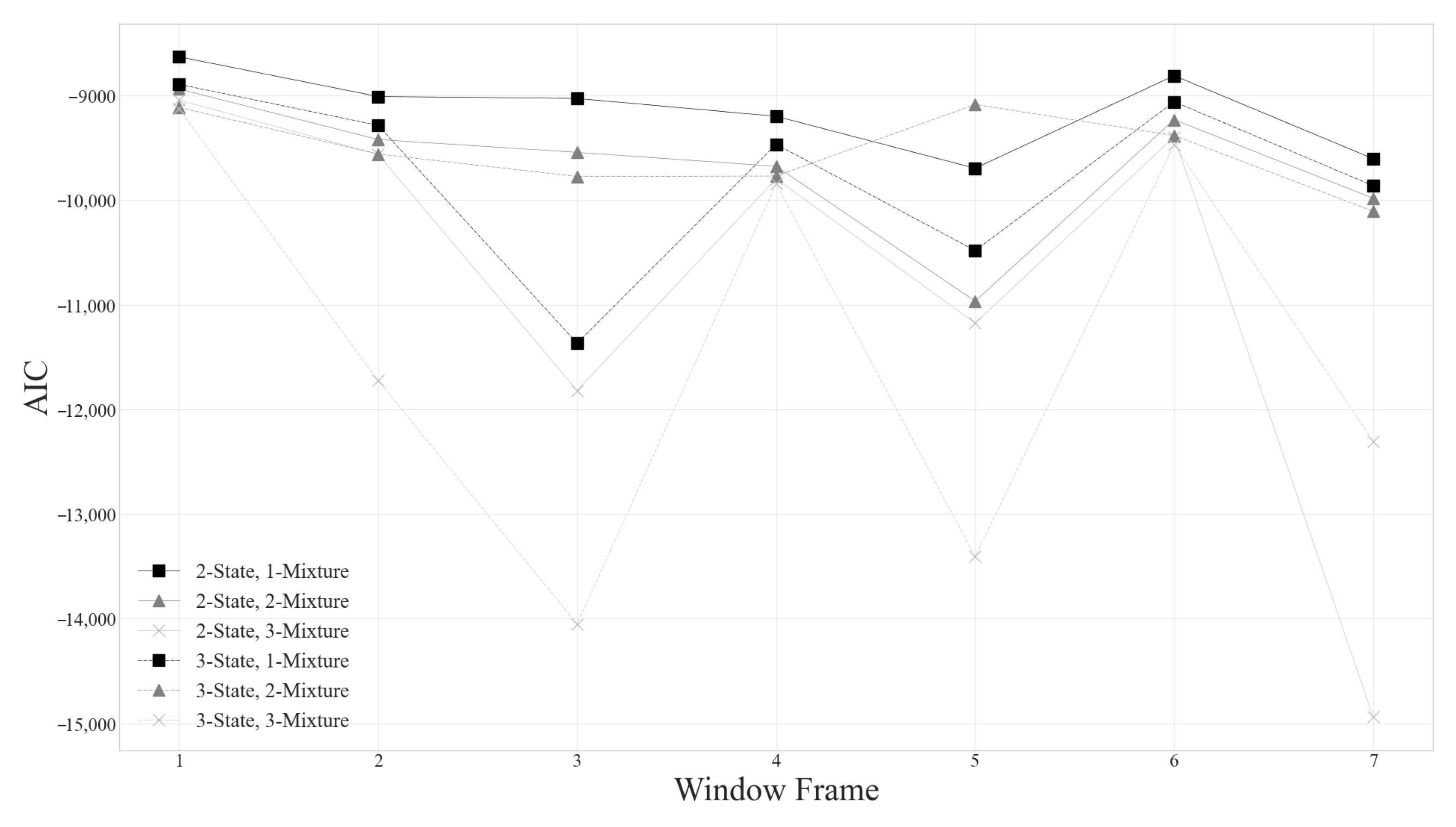
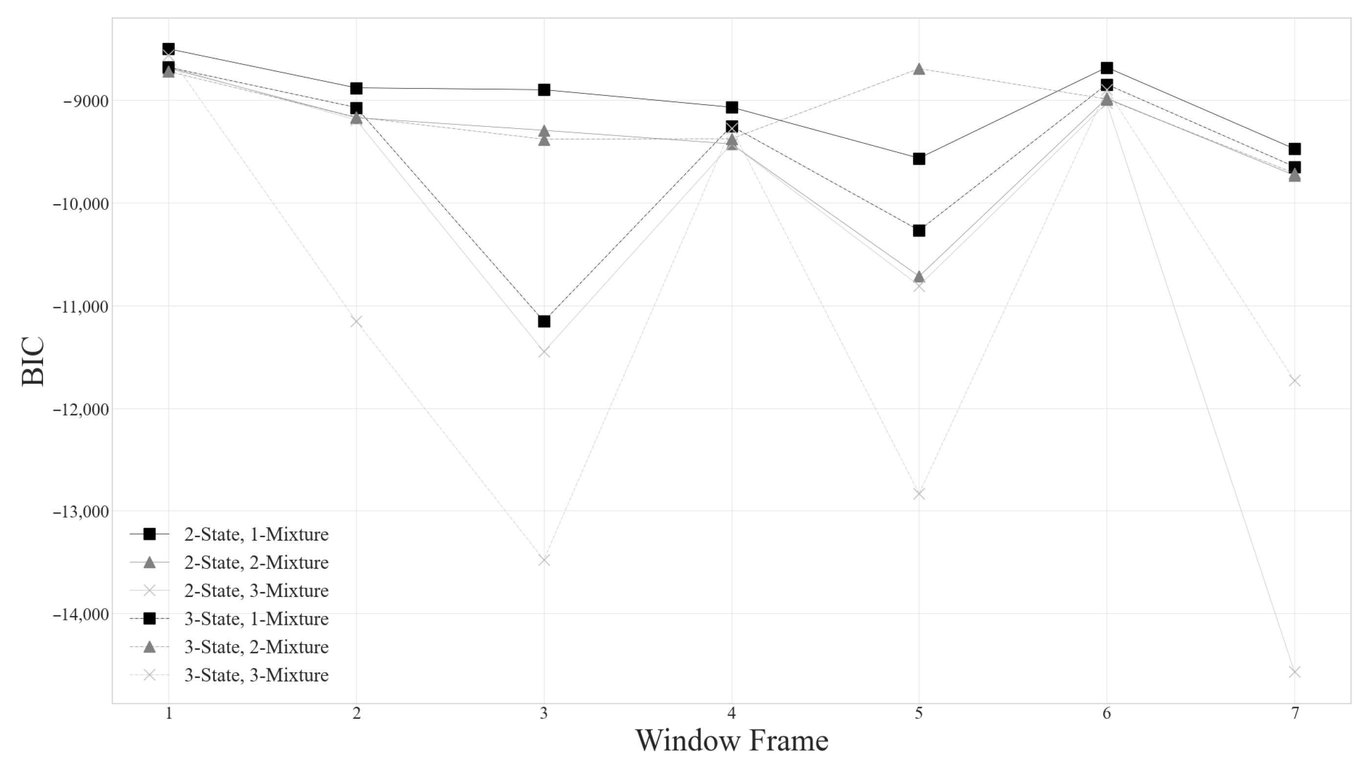
Figure 1 and Figure 2 present the AIC and BIC values for gmHMMs with two to three hidden states and one to three components applied to 2923 records of industry-level security. Each window frame spans 255 trading days, equivalent to approximately one year. The results indicate that the number of components (M) has a significantly greater influence on the model than the number of hidden states (N). The optimal model, yielding the lowest AIC and BIC values, comprises three components; subsequently, models with two components and one component exhibit increasing AIC and BIC values, respectively.

The experimental results indicate that the gmHMM model comprising three hidden regimes (N = 3) and three components (M = 3) exhibits the lowest AIC and BIC values. Consequently, this model is employed to analyze the parameters of the sectoral stock index in subsequent steps. The suitability of a multivariate model with three hidden regimes and three components suggests that the logistics sector index encompasses bullish and bearish market conditions and a sideways (neutral) market condition. Furthermore, the observation that the output signal consists of three components indicates that the observed signal ${\mathrm{O}}_{\mathrm{t}}$ does not follow a normal distribution but rather a multivariate Gaussian mixture distribution. This empirical evidence challenges the conventional financial theory, which often assumes a Gaussian distribution for such signals.

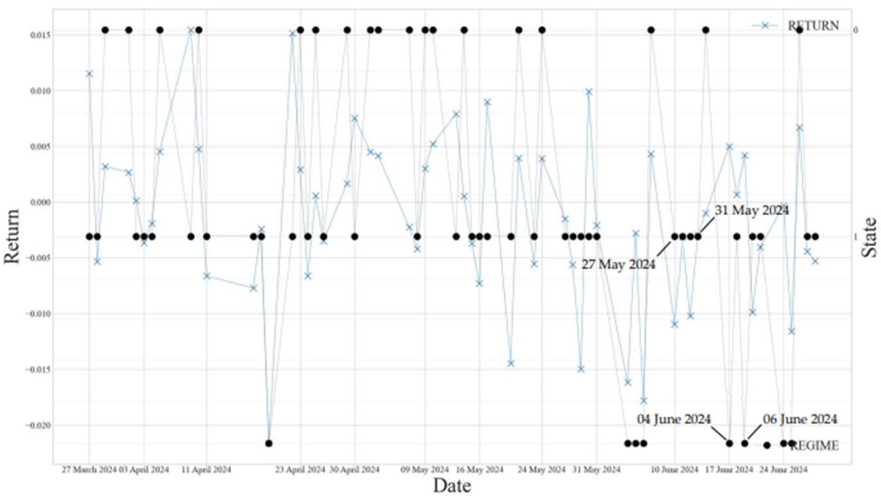
Figure 3 illustrates the returns ${\mathrm{r}}_{\mathrm{OC}}$ of the sectoral stock index categorized by hidden regimes over the last 60 days. States represent the three hidden regimes numbered 0 to 2. State 0 predominantly features positive ${\mathrm{r}}_{\mathrm{OC}}$, indicating a bullish market condition. State 1 corresponds to a sideways market, where returns are neither consistently positive nor consistently negative. State 2 indicates the bearish market condition. For example, between 27 and 31 May, the market showed significant negative returns on 29 May, which may appear to represent a bearish market. However, the gmHMM model identifies this period as a sideways market. On the following day, on 30 May, ${\mathrm{r}}_{\mathrm{OC}}$ rebounded sharply to 0.001, seemingly indicating a return to a bullish market. Nonetheless, the model continued to classify the market as sideways rather than bullish. Subsequently, from 4 June to 6 June, the market transitioned to a bearish condition. The ability of the gmHMM model to accurately predict market states proves highly beneficial for investors’ decision-making, as it discourages decisions based on single time points. Instead, the model emphasizes the importance of probability-based decision-making.

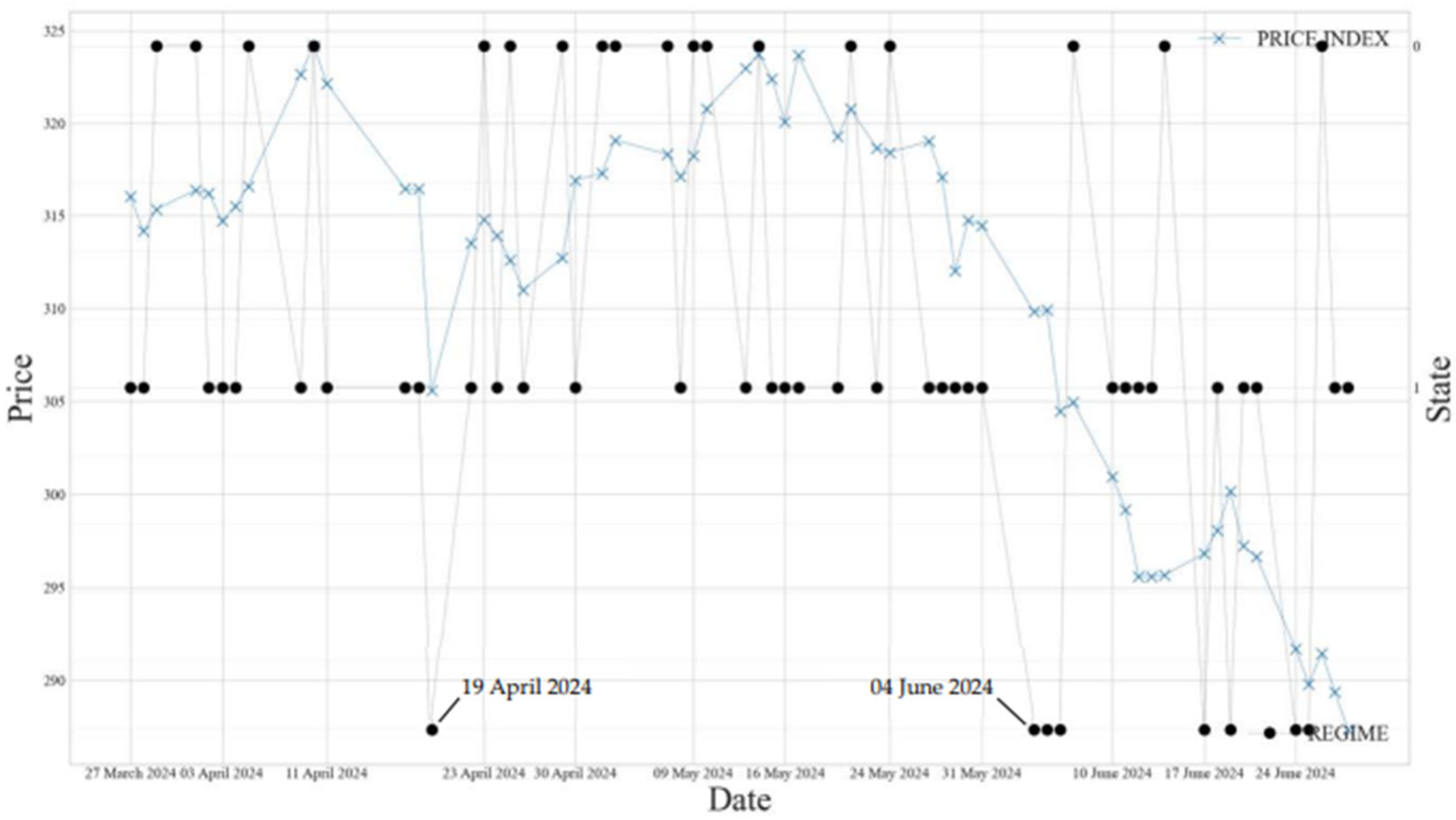
Figure 4 illustrates that the hidden regimes effectively categorize the logistics sector index into three distinct groups. Bearish market signals first emerged on 19 April, when the index dropped to 305, marking the onset of bearish conditions that would develop on 4 June. The index decline on that date corresponds to the ${\mathrm{r}}_{\mathrm{OC}}$ values shown in Figure 3. The gmHMM model’s ability to detect hidden regimes in the stock index provides valuable insights for investors and stakeholders, helping to mitigate potential wealth losses during bearish market periods.

Unlike conventional time-series models that assume global stationarity, the hidden Markov model framework is inherently suitable for nonstationary processes. In this study, we intentionally retain structural variability across time and allow the model to infer latent regimes based on shifts in the observed return distributions. Pre-testing for stationarity may constrain the model’s ability to capture genuine regime changes and is therefore omitted.

Given the unsupervised nature of the hidden Markov model, the true latent states are not observable. Consequently, traditional residual diagnostics or posterior accuracy assessments are not applicable. Instead, model evaluation is conducted using AIC and BIC, and regime-specific distributions are examined to assess behavioral consistency across states.

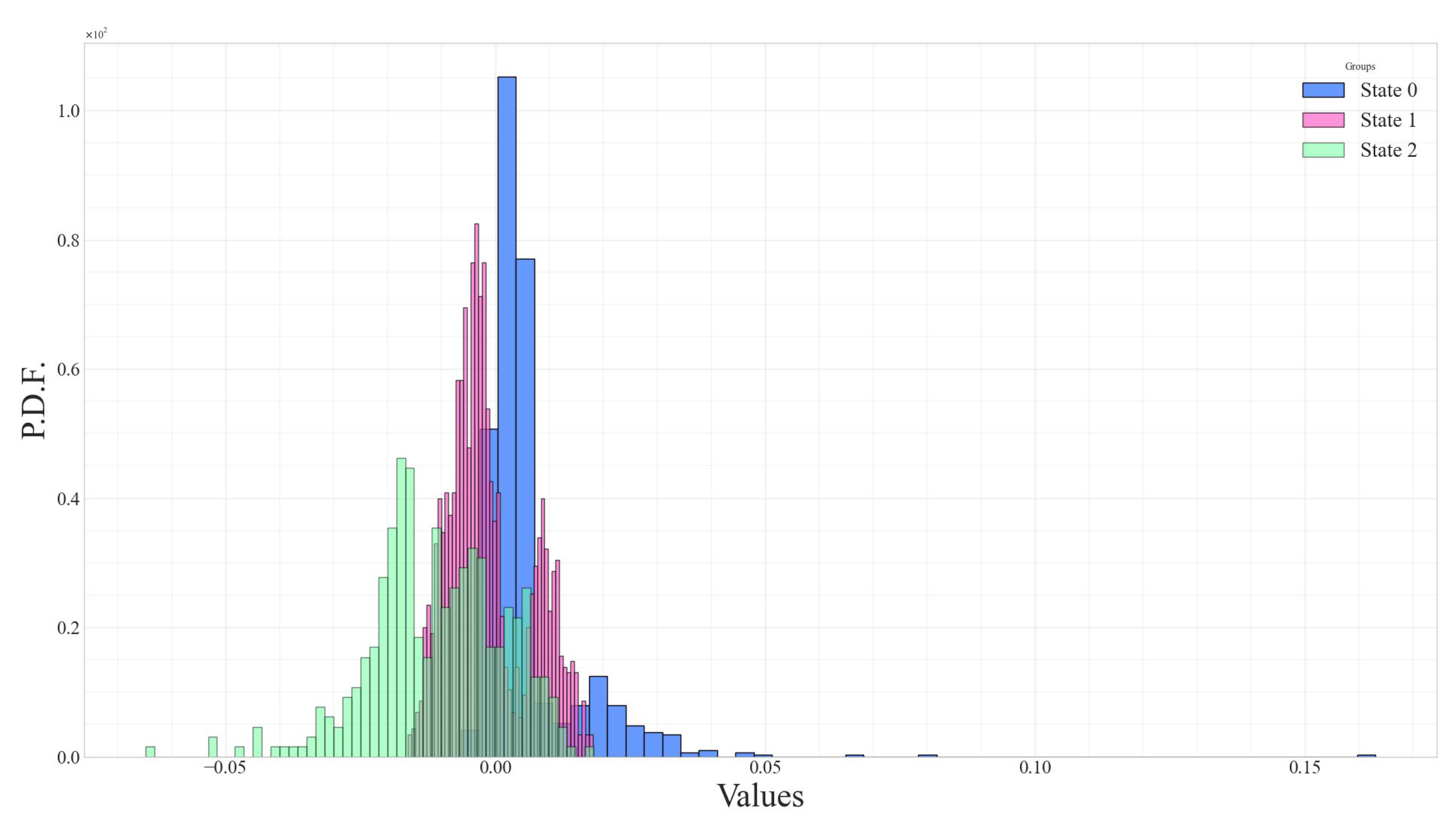
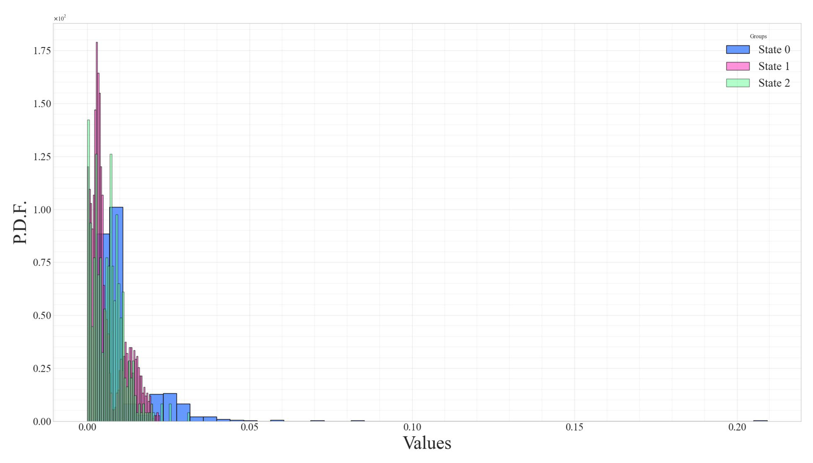
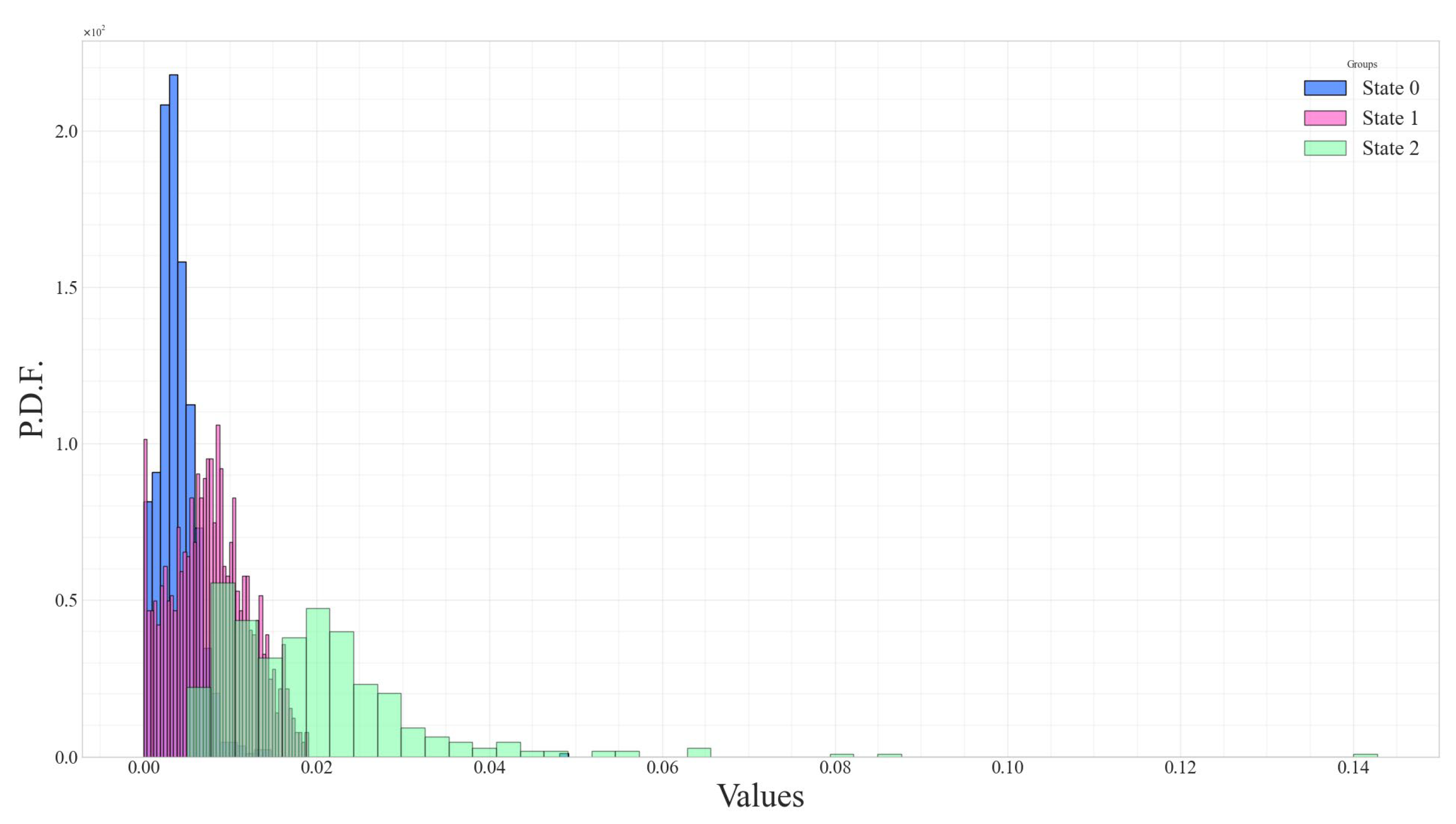
The distributions of returns, namely ${\mathrm{r}}_{\mathrm{OC}}$, ${\mathrm{r}}_{\mathrm{OH}}$, and ${\mathrm{r}}_{\mathrm{OL}}$, are shown as histograms in Figure 5, Figure 6 and Figure 7, respectively. States 0, 1, and 2 represent bullish, sideways, and bearish market conditions. These return distributions deviate from a standard Gaussian form and instead follow a Gaussian mixture distribution, consistent with the gmHMM model assumption.

Each return metric captures a different aspect of price movement. ${\mathrm{r}}_{\mathrm{OC}}$ reflects same-day returns from open-to-close, while ${\mathrm{r}}_{\mathrm{OH}}$ and ${\mathrm{r}}_{\mathrm{OL}}$ denote intraday returns from open to high and low to open, respectively, which are inherently non-negative. Although the gmHMM model assumes that the observation vector ${\mathrm{O}}_{\mathrm{t}} = ({\mathrm{r}}_{\mathrm{OC}},{\mathrm{r}}_{\mathrm{OH}},{\mathrm{r}}_{\mathrm{OL}})$ follows a Gaussian mixture distribution that allows both positive and negative values, this assumption may conflict with the nature of ${\mathrm{r}}_{\mathrm{OH}}$ and ${\mathrm{r}}_{\mathrm{OL}}$. This study is the first to explicitly address this limitation, which was not previously discussed in works such as Gupta and Dhingra (2012). Nevertheless, using ${\mathrm{O}}_{\mathrm{t}}$ as a feature for regime detection may enhance the stationarity of the time series and improve model performance.

Table 1. Descriptive statistics and Kruskal–Wallis H-statistics for return parameters $\left({\mathrm{r}}_{\mathrm{OC}},{ \mathrm{r}}_{\mathrm{OH}},{ \mathrm{r}}_{\mathrm{OL}}\right)$, volume, and open interest (OI) across hidden regimes identified by the 3-state, 3-mixture gmHMM.

	${\mathbf{r}}_{\mathbf{OC}}$				${\mathbf{r}}_{\mathbf{OH}}$					${\mathbf{r}}_{\mathbf{OL}}$
State	0	1		2	0		1		2	0		1		2
Count	850	1682		391	850		1682		391	850		1682		391
Mean	0.0062	−0.0013		−0.0108	0.0111		0.0059		0.0065	0.0038		0.0077		0.0198
Std	0.0103	0.0076		0.0124	0.0111		0.0052		0.0049	0.0026		0.0044		0.0127
Min	−0.0063	−0.0162		−0.0648	0.0027		0.0000		0.0000	0.0000		0.0000		0.0050
25%	0.0010	−0.0066		−0.0186	0.0060		0.0023		0.0027	0.0023		0.0044		0.0114
Median	0.0035	−0.0030		−0.0107	0.0078		0.0038		0.0063	0.0035		0.0076		0.0182
75%	0.0060	0.0045		−0.0020	0.0101		0.0096		0.0092	0.0050		0.0107		0.0236
Max	0.1630	0.0180		0.0182	0.2092		0.0222		0.0314	0.0491		0.0190		0.1428
Skew	5.7885	0.5418		−0.5101	8.0068		1.0839		1.1418	6.4160		0.2105		3.6752
Kurtosis	67.7792	−0.6247		0.8372	122.4505		0.0045		2.4465	101.7635		−0.6266		25.9870
CV	1.6746	−5.9624		−1.1545	1.0004		0.8828		1.1418	0.6934		0.5727		0.6410
ES	−0.0026	−0.0132		−0.0398	0.0037		0.0002		0.0001	0.0001		0.0002		0.0064
MaxDD	−0.0063	−0.8942		−0.9858	-		-		-	-		-		-
H-Stat	711.8005				418.1601					1134.4331
p-value	0.0000				0.0000					0.0000
	Volume							OI
State	0		1			2		0			1		2
Count	850		1682			391		850			1682		391
Mean	306,663		301,087			356,559		3,284,837			3,240,941		4,334,220
Std	264,616		237,193			258,761		2,066,545			1,701,159		2,843,315
Min	45,989		49,716			71,173		314,618			377,701		1,075,968
25%	162,993		165,111			191,402		2,047,673			2,099,357		2,531,280
Median	228,751		241,192			293,832		2,852,376			2,880,389		3,628,757
75%	343,797		353,561			429,040		3,861,833			3,964,270		5,228,287
Max	2,614,801		3,681,549			2,490,096		27,839,883			14,632,402		28,816,659
Skew	3.7893		4.4408			3.1615		3.8283			1.8144		3.3046
Kurtosis	21.1804		37.4143			16.6636		30.1095			5.7111		20.3528
H-Stat	35.3458							72.4824
p-value	0.0000							0.0000

Note: This table presents the mean, standard deviation, skewness, and kurtosis of each parameter across hidden regimes. The Kruskal–Wallis H-statistic and corresponding p-value indicate statistically significant differences among regimes (p < 0.05). Maximum drawdown (MaxDD) is only applicable to ${\mathrm{r}}_{\mathrm{OC}}$, which represents a cumulative return series. For ${\mathrm{r}}_{\mathrm{OH}}$ and ${\mathrm{r}}_{\mathrm{OL}}$, which are intraday directional returns, drawdown is not defined.

provides a comprehensive comparison of descriptive statistics, distributional properties, and risk indicators across the three hidden regimes identified by the gmHMM. Notably, regime 2—characterized as the bearish regime—exhibits the lowest average return (–1.08%), the highest standard deviation (1.24%), and a strongly negative expected shortfall (ES = –3.98%). The maximum drawdown (MaxDD) in this regime reaches –98.58%, reinforcing its status as a high-risk environment.

In contrast, regime 0 (bullish) exhibits a relatively stable risk–return profile, characterized by a positive average return (0.62%) and limited downside exposure (ES = –0.26%, MaxDD = –0.63%). The coefficient of variation (CV) further distinguishes the risk efficiency of each regime. Specifically, regime 1 (sideways) exhibits a negative mean but moderate volatility, resulting in an extreme negative CV (–5.96), which indicates an inefficient risk-adjusted profile.

These empirical findings support the interpretation that incorporating hidden regime detection into portfolio management can enhance risk control by identifying latent high-risk states that are not captured through traditional return-based indicators. Consequently, regime-aware strategies may contribute to better drawdown mitigation and improved capital preservation during adverse market conditions.

The descriptive statistics of the histograms shown in Figure 5, Figure 6 and Figure 7 are summarized in Table 1, demonstrating that the distributions of the elements in the ${\mathrm{O}}_{\mathrm{t}}$ vector do not follow a normal distribution. The skewness values range from −0.5101 to 8.0068, while the kurtosis values range from −0.6266 to 122.4505, significantly differing from the skewness and kurtosis values of a Gaussian distribution, which are 0 and 3, respectively. As a result, statistical testing for the distributions of ${\mathrm{r}}_{\mathrm{OC}}$, ${\mathrm{r}}_{\mathrm{OH}}$, and ${\mathrm{r}}_{\mathrm{OL}}$ values across different hidden regimes necessitates using non-parametric tests, such as the Kruskal–Wallis test.

The H-statistics and p-values from the Kruskal–Wallis test indicate that the distribution of the observed signal ${\mathrm{O}}_{\mathrm{t}}$ depends on the hidden regimes. The p-values for the tests on ${\mathrm{r}}_{\mathrm{OC}}$, ${\mathrm{r}}_{\mathrm{OH}}$, and ${\mathrm{r}}_{\mathrm{OL}}$ are less than 0.05, leading to the rejection of ${\mathrm{H}}_0$. This confirms that the distributions of the three-return metrics differ significantly statistically. Consequently, the observed signal ${\mathrm{O}}_{\mathrm{t}}$, represented as a vector comprising ${\mathrm{r}}_{\mathrm{OC}}$, ${\mathrm{r}}_{\mathrm{OH}}$, and ${\mathrm{r}}_{\mathrm{OL}}$, can serve as a reliable proxy for the hidden regimes in the industry-level equity index. The results reveal substantial heterogeneity in the statistical properties across regimes, confirming the model’s ability to distinguish economically meaningful latent states.

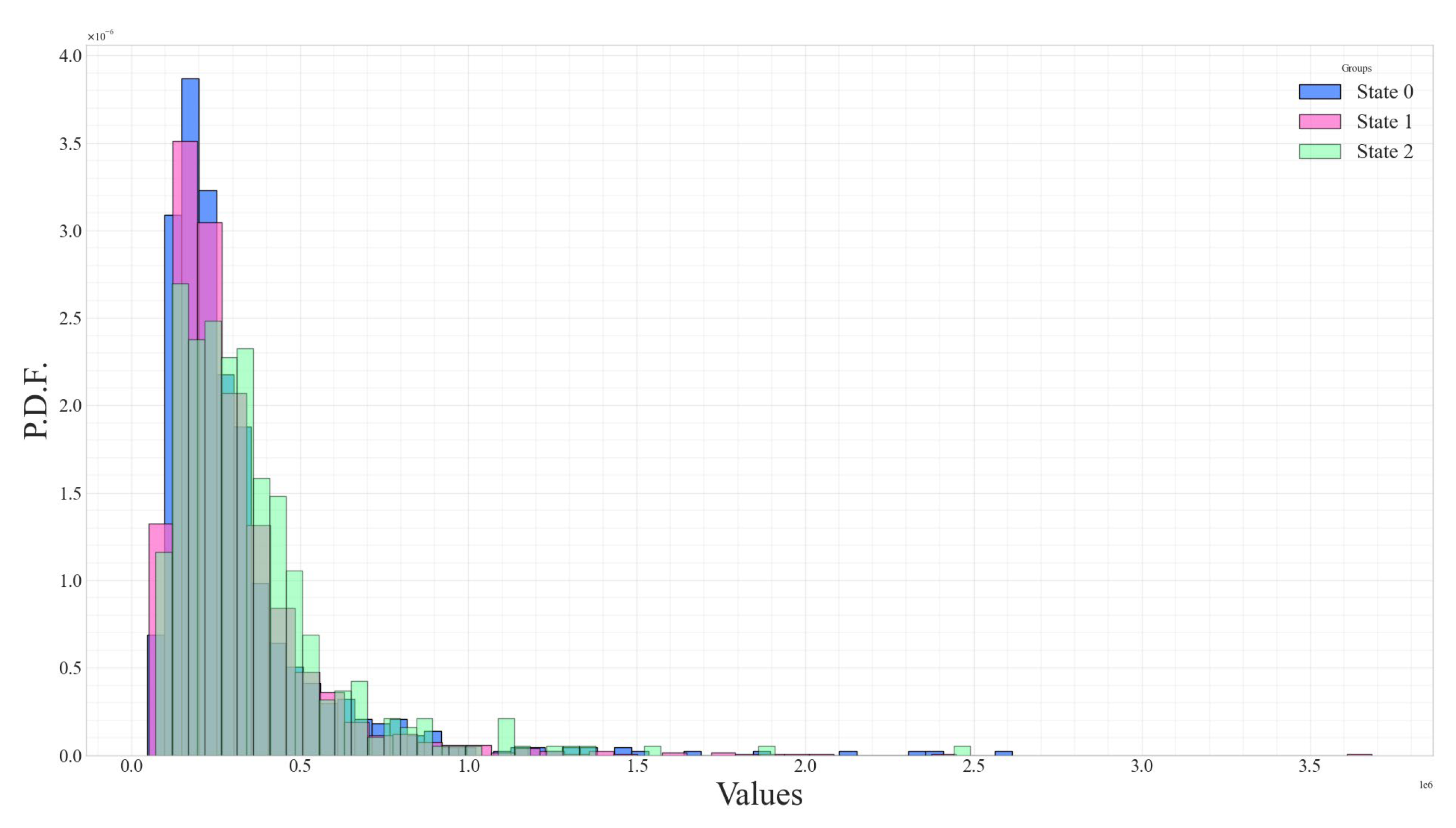
Figure 8 and Figure 9 display the distributions of volume and open interest (OI) for the sectoral sector stock index, along with daily data points and OHLC prices. These figures show that volume and OI exhibit distinct distributions across different hidden regimes. Table 1 presents the descriptive statistics and results of the Kruskal–Wallis tests for these two parameters. The findings confirm that the distributions of volume and OI differ significantly across the hidden regimes, demonstrating statistical significance.

The bearish market condition, State 2, exhibits a significantly higher trading volume than the other two states. The trading volume during the bearish market reached 356,559, compared to 306,663 and 301,087 in the bullish and sideways market states. The elevated trading volume in the bearish market suggests that investors experienced heightened panic, leading to an abnormal increase in transaction activity.

Open interest (OI) also increased abnormally during the bearish market, reaching 4,334,220 compared to 3,284,837 and 3,240,941 in the bullish and sideways market states. The elevated OI indicates that investors are engaging more in derivative markets and opening positions at a higher rate. When considered alongside the declining ${\mathrm{r}}_{\mathrm{OC}}$ values and rising trading volume, which reflects heightened panic among investors during the bearish market conditions. This behavior aligns with the literature that associates regime shifts with structural breaks in market sentiment and liquidity conditions.

While volume and open interest are not direct inputs into the gmHMM, their distributions across hidden states are analyzed post-estimation. Notably, extreme OI values are concentrated in bearish regimes, indicating that derivative-based positioning activity may intensify during market stress. Nevertheless, these variables alone do not provide sufficient information for standalone regime identification.

The experimental results using the designed gmHMM model confirm the presence of hidden regimes underlying the daily index of sectoral stocks. These hidden regimes significantly influence the distributions of observable signals, such as ${\mathrm{r}}_{\mathrm{OC}}$, ${\mathrm{r}}_{\mathrm{OH}}$, ${\mathrm{r}}_{\mathrm{OL}}$, volume, and OI. The Kruskal–Wallis test validates the differences in the distributions of these five parameters, with p-values < 0.05. Therefore, these parameters can serve as proxies for identifying the hidden regimes, particularly volume and OI, which exhibit abnormal increases during bearish market conditions. The daily mean values of ${\mathrm{r}}_{\mathrm{OC}}$, ${\mathrm{r}}_{\mathrm{OH}}$, and ${\mathrm{r}}_{\mathrm{OL}}$ during the bearish state, as presented in Table 1, are −0.0108, 0.0065, and 0.0198, respectively. This highlights the distinct characteristics of the bearish market condition compared to other regimes.

Overall, the integration of regime-specific risk measures (e.g., ES and MaxDD) provides investors with a deeper understanding of the sector’s latent risk dynamics. The findings underscore the importance of regime-aware portfolio design, particularly in industries that exhibit non-linear responses to macroeconomic and sentiment shifts. Adaptive strategies incorporating hidden regime signals may enhance capital preservation and reduce exposure during unfavorable market phases.

5. Discussions

The empirical findings from the gmHMM reveal three distinct latent regimes that reflect the underlying dynamics in the logistics sector of the Thai equity market. These regimes are inferred endogenously from return distributions and volatility profiles, rather than imposed through exogenous macroeconomic variables.

Table 2. Risk regime interpretation and strategic investment implications.

Regime (State)	Market Behavior	Interpretation	Strategic Implication
State 0	Low volatility with moderate positive return	Reflects a stable growth phase with limited downside risk and consistent performance across multiple return measures.	Favorable for long positions, particularly in sectoral accumulation or passive strategies.
State 1	Moderate volatility with slightly negative or flat return	Indicates a transitional state with uncertain direction, possibly reflecting market indecision or mild correction.	Suggests a risk-neutral stance, reducing exposure or reallocating assets temporarily.
State 2	High volatility with negative return and severe drawdowns	Represents a crisis or high-risk regime, marked by elevated tail risk and market distress.	Calls for defensive strategies, such as hedging, de-risking, or short positioning.

encapsulates these latent structures across three return signals—open-to-close, open-to-high, and low-to-open—and provides regime-specific downside risk metrics.

Regime 0 is characterized by low volatility, moderate positive returns, and favorable downside risk statistics. The close-to-open return exhibits a mean of 0.0062, with a standard deviation of 0.0103, accompanied by minimal expected shortfall (−0.0026) and a max drawdown of −0.0063. These statistical features correspond to a tranquil market environment, aligning with the notion of equilibrium risk pricing as proposed by Merton (1973). The Gaussian mixture components display low excess kurtosis and subdued skewness, reinforcing the interpretation of this regime as a risk-neutral holding phase. In practical terms, this regime supports buy-and-hold or volatility-targeted strategies. Neal et al. (2024) reinforced this interpretation by demonstrating that panel-based HMMs can capture low-volatility, high-persistence regimes in equity subsectors with homogeneous exposure. Their findings validate the existence of stable regimes that evolve slowly over time, particularly in sectors such as logistics, where firm operations are capital-intensive and exhibit predictable cyclical patterns.

Regime 1 exhibits the lowest volatility among all regimes (σ = 0.0076), characterized by near-zero average returns. Though this state exhibits platykurtic distributions and minimal skew, its prevalence—occupying 57.5% of the entire sample—signifies a dominant mode of market behavior. The subdued return performance and narrow distribution suggest a state of uncertainty or transition. This aligns with scenarios where investors are digesting new information, particularly policy signals or global supply chain shocks. In such conditions, directional strategies are inefficient, and mean reversion or statistical arbitrage may offer greater efficacy. This regime exemplifies the dynamics described by Lenart et al. (2024), whose nonlinear stationary regime model with frequency decomposition identifies periods of dampened oscillations coinciding with latent economic stagnation. Their findings support the view that certain states represent neither clear expansion nor contraction but instead reflect informational adjustment in financial markets.

Regime 2 signifies the most turbulent environment, displaying the highest volatility and most adverse risk characteristics. With a negative mean return (−0.0108), extreme expected shortfall (−0.0398), and significant drawdown (−0.9858), this regime is indicative of crisis behavior. Skewness is notably negative, and kurtosis is elevated, reflecting heavy tails and asymmetry in returns. The substantial surge in trading volume and open interest during this state confirms elevated uncertainty and strategic hedging behavior. These conditions are consistent with Hamilton’s (1989) canonical interpretation of recessionary regimes in financial time series. Furthermore, the multivariate unobserved components model presented by Jahan-Parvar et al. (2024) provides empirical evidence that volatility clustering and synchronized return collapses are reliably detected via Bayesian filters in high-frequency data. Their approach supports the identification of such latent downturn states in sector-specific indices.

The modeling strategy adopted in this study leverages high-frequency, multivariate price data to reveal latent economic behavior without the need for exogenous indicators. This finding is consistent with the results of Catello et al. (2023), who apply HMMs to equity indices and demonstrate that models using only observable price series can successfully classify the states of market turbulence, stability, and transition. Their results highlight that investor-relevant features, such as return asymmetry and kurtosis, can be effectively modeled using Gaussian mixtures.

In integrating deep learning approaches, Sivakumar (2025) proposes an HMM–LSTM fusion that confirms the complementarity of probabilistic regime modeling with neural predictive engines. Though the current study maintains a fully probabilistic formulation, future research could incorporate similar hybrid methods to enhance temporal pattern recognition in latent regimes. Finally, the foundational review by Manjunatha et al. (2024) consolidates theoretical justifications for gmHMMs in financial domains, particularly emphasizing their superiority over standard HMMs in handling non-Gaussian, multivariate data distributions. Their synthesis supports the structural design adopted in this study and validates the use of Gaussian mixtures in sector-specific risk modeling.

By aligning these empirical patterns with theoretical constructs and recent literature, the discussion reveals how each regime contributes distinctively to the interpretation of risk and the formation of investment strategies. The observed regimes map clearly onto actionable investor behavior: volatility targeting and passive holding in Regime 0; statistical arbitrage in Regime 1; and capital preservation and hedging in Regime 2. The insights extend the regime-switching theory by validating its application at the sectoral index level in emerging markets—a domain often underrepresented in the existing literature.

Unlike prior studies that focused on macro-level regime identification using monthly or quarterly economic indicators (Nguyen and Nguyen 2015, 2021; Kritzman et al. 2012), this study derives latent regime signals from daily price movements and trading activity within a sectoral index. The findings reveal that observable metrics, such as volume and open interest, are statistically associated with hidden regimes. This insight enables practitioners to monitor regime shifts using accessible, real-time data, particularly relevant in emerging markets where computational resources and data transparency may be limited. Moreover, the model facilitates early detection of adverse risk regimes, allowing for capital preservation and informed portfolio rebalancing strategies, especially during periods of market dislocation.

The logistics sector (TRANS) was selected due to its pronounced sensitivity to both domestic economic policy and global trade flows, making it an ideal candidate for capturing the regime-switching behavior. Its volatility and responsiveness to supply chain disruptions offer a clear testing ground for models designed to detect latent state transitions. While this study focuses on a single sector within a single market, the modeling framework is flexible and may be extended to other industries or countries. Future research could investigate the robustness of the gmHMM framework across sectors with varying structural characteristics to assess the generalizability of the results.

Beyond statistical classification, the latent regimes identified by the gmHMM framework can also be interpreted through the lens of temporal policy anchoring. For instance, the high-volatility regime (State 2), which emerged during specific sub-periods, corresponds with macroeconomic stress events, such as the 2013 Thai political unrest, the COVID-19 outbreak in 2020, and the global supply chain crisis in 2021–2022. These episodes coincide with sharp movements in the logistics sector index and elevated open interest, reflecting both uncertainty and delays in policy responses. Conversely, the low-volatility regime (State 0) tends to align with periods of monetary easing, fiscal stimulus, and trade stabilization policies enacted during 2017–2018 and post-COVID recovery phases in 2023. These alignments suggest that the inferred regimes may implicitly reflect investor expectations and market reactions to temporal policy shifts, even in the absence of explicit exogenous variables. Integrating economic timelines into interpretation reinforces the economic relevance of the latent states and provides a bridge between statistical modeling and macro-financial narratives in emerging markets.

This study confirms the existence of hidden regimes in the logistics sector index within the SET50 index of the Stock Exchange of Thailand. It successfully identifies proxies capable of indicating the daily hidden regimes embedded in the index. Investors and stakeholders can adjust their investment strategies to align with the unobservable hidden regimes. Enhanced long-term investment performance in the sectoral stock index can be anticipated by applying the gmHMM model, as demonstrated in this research.

The academic contribution of this study lies in extending the interpretability and applicability of regime-switching models in several important ways. First, the study enhances the transparency of latent regime behavior through visualized return distributions, allowing for an intuitive understanding of market phases. Second, it operationalizes regime-specific downside risk metrics—namely expected shortfall and maximum drawdown—that directly link latent states to investor-relevant risk indicators. Third, by applying a multivariate gmHMM to high-frequency, sector-specific data in an emerging market context, the study expands the scope of unsupervised learning methods beyond aggregate market indices to the meso-level of industry dynamics.

6. Materials and Methods

The experimental design was developed to directly address the research objectives stated in the introduction. These include identifying the number of latent regimes in the sectoral stock index, determining the optimal number of Gaussian mixture components for each return feature, and characterizing regime-specific behavior in terms of return distributions and downside risk.

6.1. Experimental Data

This study utilizes daily time series data of the logistics sector index from the Stock Exchange of Thailand, covering the period from 2 July 2012, to 28 June 2024, with a total of 2923 observations. The dataset was retrieved from the ASPEN Desktop platform, developed by ThaiQuest Limited, based in Bangkok, Thailand. The dataset includes Open, High, Low, and Close prices, as well as trading volume and open interest data specific to the logistics sector index, recorded for each trading day.

6.2. Experimental Method

The experiment was designed to address three research questions: (1) identifying the number of hidden regimes, (2) determining the number of observable signal components in the model, and (3) analyzing returns and volatility within each hidden regime.

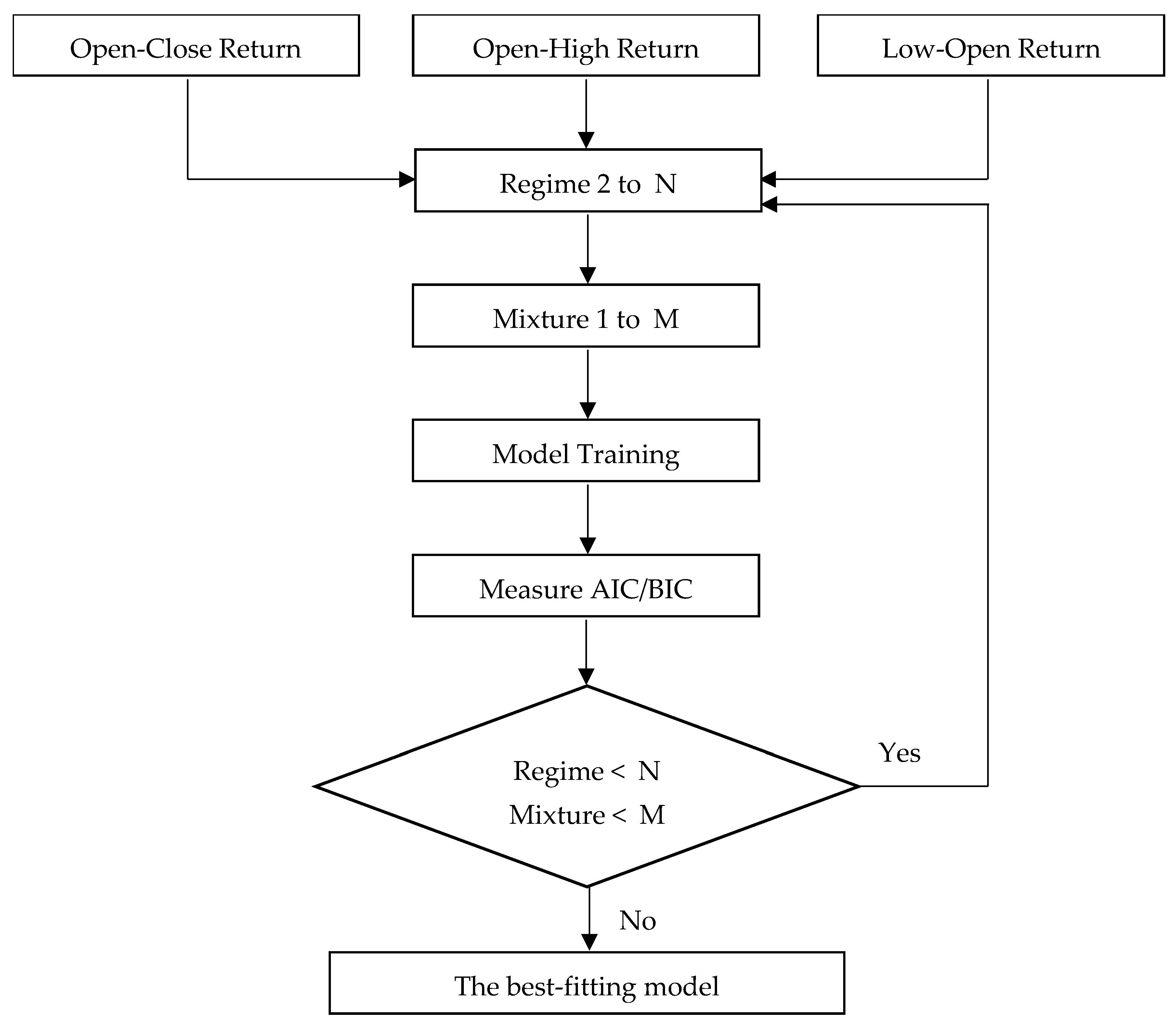
Initially, a gmHMM was constructed to best fit the dataset, guided by Akaike Information Criterion (AIC) and Bayesian Information Criterion (BIC) values. Various models with differing numbers of hidden regimes and components were evaluated. The model yielding the lowest AIC and BIC was selected to identify hidden regimes, followed by an analysis of returns and volatility. The modeling process is illustrated in Figure 10.

The gmHMM model was developed through an iterative process, where the number of hidden regimes varied from 2 to $\mathrm{N}$ and the number of mixture components from 1 to M, resulting in a total of $(\mathrm{N}-1) \times \mathrm{M}$ model configurations. In this study, we specifically selected N and M to be three. Choosing between two and three hidden regimes enabled us to represent different market conditions: two regimes correspond to bullish and bearish markets (N = 2), while a three-regime model introduces a neutral state (N = 3). Notably, the one-regime models with two or three mixtures are equivalent to the two-regime and three-regime univariate gmHMMs, respectively. The optimal gmHMM model was selected based on the lowest AIC and BIC values among the six configurations.

Subsequently, the observed signal ${\mathrm{O}}_{\mathrm{t}}$ (1) of the sectoral stock index is input into the constructed gmHMM model. The Viterbi algorithm identifies the hidden regimes present in the daily data. The distributions of ${\mathrm{r}}_{\mathrm{OC}}$, ${\mathrm{r}}_{\mathrm{OH}}$, and ${\mathrm{r}}_{\mathrm{OL}}$ values across different hidden regimes are analyzed and tested to confirm that the hidden regimes produce distinct output signals. The Kruskal–Wallis test, a non-parametric method, is employed to validate the differences in output signals among the various hidden regimes.

Section 4 reports the model selection results based on AIC and BIC for all six configurations. In addition, non-parametric statistical testing is applied to examine whether the distributions of ${\mathrm{r}}_{\mathrm{OC}}$, ${\mathrm{r}}_{\mathrm{OH}}$, and ${\mathrm{r}}_{\mathrm{OL}}$ differ significantly across the inferred regimes. These tests support the interpretation of distinct regime-specific return behaviors and help evaluate the effectiveness of observable variables as proxies for hidden state transitions.

The regime-tagged observations were subjected to further statistical analyses to characterize downside risk in each state. Metrics, including expected shortfall (ES), maximum drawdown (MDD), and coefficient of variation (CV), were computed separately for each regime to quantify their risk–return profiles. This regime-aware risk profiling facilitates an understanding of how risk exposure varies across different market conditions. It aligns with theoretical frameworks, such as Merton’s (1973) intertemporal capital asset pricing model (ICAPM) and regime-switching consumption-based asset pricing models.

This modeling strategy aligns with recent empirical advances in combining latent state models with high-dimensional return structures (Neal et al. 2024; Catello et al. 2023). In the context of an emerging market sectoral index, gmHMM offers a nuanced tool for detecting latent regimes and associating them with economically meaningful behaviors and policy phases. The methodological rigor and interpretability of the gmHMM framework make it particularly suitable for studying regime-dependent phenomena in financial markets characterized by structural nonlinearity and time-varying risk preferences.

7. Conclusions

This study applied a multivariate Gaussian mixture hidden Markov model (gmHMM) to identify latent regimes in the logistics sector of the Thai equity market. By incorporating intraday return vectors alongside volume and open interest, the model captured structural patterns in return dynamics and trading activity that are often obscured in traditional analyses. The regime identification process was entirely data-driven, enabling endogenous detection of market phases without reliance on exogenous economic labels.

The empirical findings revealed three statistically and behaviorally distinct regimes: a bullish state characterized by stable returns and minimal downside risk, a transitional state marked by low volatility and stagnation in returns, and a bearish state characterized by heightened volatility, significantly negative returns, and severe drawdowns. These differentiated risk–return profiles provide practical insights for regime-aware asset allocation, emphasizing the importance of monitoring latent states in dynamic market environments.

From a strategic standpoint, the gmHMM framework supports early risk detection and informs adaptive investment strategies, particularly in emerging markets where conventional indicators may be delayed or unreliable. Academically, this study contributes to the literature by extending the interpretability of hidden market regimes through the integration of trading activity variables and by operationalizing regime-specific downside risk metrics. These enhancements advance the methodological toolkit for financial regime analysis and deepen the practical relevance of unsupervised learning models in sector-specific equity research. However, limitations remain: the framework assumes Gaussian mixture distributions and relies on random initialization, which may affect local convergence. These aspects suggest future research directions involving more flexible distributional assumptions and enhanced initialization techniques to improve the model’s robustness and generalizability. In addition, subsequent studies could incorporate quantitative backtesting of regime-aligned investment strategies to validate the model’s utility empirically. Such extensions would enable direct performance comparisons with conventional risk-based or momentum-driven portfolio allocation methods, thereby strengthening the practical relevance of the gmHMM framework in applied financial decision-making.