Abstract
Over the past decade, multifactor models have shown enhanced capability compared to single-factor models in explaining asset return variability. Given the common assertion that higher risk tends to yield higher returns, this study empirically examines the augmented human capital six-factor model’s performance on thirty-two portfolios of non-financial firms sorted by size, value, profitability, investment, and labor income growth in the Indian market over the period July 2010 to June 2023. Moreover, the current study extends the Fama and French five-factor model by incorporating a human capital proxy by labor income growth as an additional factor thereby proposing an augmented six-factor asset pricing model (HC6FM). The Fama and MacBeth two-step estimation methodology is employed for the empirical analysis. The results reveal that small-cap portfolios yield significantly higher returns than large-cap portfolios. Moreover, all six factors significantly explain the time-series variation in excess portfolio returns. Our findings reveal that the Indian stock market experienced heightened volatility during the COVID-19 pandemic, leading to a decline in the six-factor model’s efficiency in explaining returns. Furthermore, Gibbons, Ross, and Shanken (GRS) test results reveal mispricing of portfolio returns during COVID-19, with a stronger rejection of portfolio efficiency across models. However, the HC6FM consistently shows lower pricing errors and better performance, specifically during and after the pandemic era. Overall, the results offer important insights for policymakers, investors, and portfolio managers in optimizing portfolio selection, particularly during periods of heightened market uncertainty.
1. Introduction
The capital asset pricing model (CAPM, hereafter) of Sharpe (1964) and Lintner (1965) has been a foundational approach in the asset pricing literature for understanding the variability in asset returns (Khan and Afeef 2024). Conceptualized as a single-factor model that incorporates only market risk, CAPM has faced substantial criticism regarding its assumptions and empirical limitations (Bhandari 1988; Friend et al. 1978; Ross 1978; Levy 1983; Roll 1977). In response to this, Ross (1976) laid the foundation of arbitrage pricing theory (APT), a multifactor model that sought to address CAPM’s shortcomings. Subsequently, Cox et al. (1985) extended the CAPM framework by incorporating savings and capital formation to enhance optimal portfolio selection. Compared to CAPM, recently developed multifactor models have demonstrated improved performance in explaining the variability in portfolio returns (Thalassinos et al. 2023). While multifactor models have improved the explanation of asset returns, they remain insufficient in fully accounting for the complexities of return behavior, highlighting the need to consider additional anomalies (Kan et al. 2024). The persistent limitations of CAPM have led scholars to identify numerous return anomalies, further highlighting the necessity for more comprehensive models in asset pricing (Harvey et al. 2016). In the financial literature, numerous researchers have identified a wide range of financial anomalies that exert a persistent influence on asset returns (Linnainmaa and Roberts 2018). For instance, Hou et al. (2020) highlighted 452 financial anomalies and documented that approximately 35% of the anomalies exhibited a statistically significant relationship with asset returns.
Over the last several decades, numerous asset pricing models have been proposed in response to these anomalies. For instance, Fama and French (1993) extended the CAPM by introducing two additional factors, namely size and value premiums, resulting in the well-known three-factor model (FF3FM, hereafter). Building upon this, Carhart (1997) incorporated a momentum factor into the FF3FM, giving rise to the four-factor asset pricing model. Later, drawing on the dividend discount model (DDM) of Miller and Modigliani (1961), Fama and French (2015) proposed a five-factor model (FF5FM) by adding investment and profitability factors to the FF3FM. Furthermore, advancing the model, Fama and French (2018) introduced a momentum-based six-factor model (FF6FM) by integrating the momentum factor into the FF5FM.
A growing body of academic literature has recognized human capital as a critical component of total wealth and a significant determinant of expected stock returns which is not fully captured by the traditional market beta (Qin 2002; Campbell 1996). Studies, such as Jagannathan and Wang (1996) and Jagannathan et al. (1998), demonstrate that incorporating human capital betas improves the explanatory power of the CAPM in both United States and Japanese markets. In emerging economies, human capital plays a vital role in addressing persistent issues, like poverty, inequality, and political instability (Amar and Pratama 2020; Wang et al. 2020; Vianna and Mollick 2018) and is considered a central driver of long-term economic growth and structural transformation (Romer 1990; Diebolt and Hippe 2019; Tridico 2007). Human capital is estimated to account for up to 90% of total wealth (Lustig et al. 2013). Recent studies, including Barras (2019), Park et al. (2021), and Roy and Shijin (2018, 2019), highlight the growing recognition of intellectual capital, namely human capital, as a key factor in the asset pricing model. Campbell (1996) highlighted that human capital represents the true wealth of the economy; therefore, this factor should be integrated into the asset pricing models. In recent years, several anomalies have been incorporated into asset pricing frameworks to capture variability in asset or portfolio returns. One critical risk-mimicking factor that remains overlooked is human capital (Prasad et al. 2024). Subsequently, several studies have demonstrated the importance of human capital in the multifactor model in the international market (Belo et al. 2017; Kim et al. 2011; Kuehn et al. 2017; Lettau et al. 2019; Khan et al. 2022; Tambosi Filho et al. 2022; Khan et al. 2023; Khan et al. 2025). Therefore, the above studies in various international markets support the human capital (HC)-based asset pricing model and confirm its superior performance in global markets. Some of the notable contributions to the six-factor multifactor model are from Shijin et al. (2012), who state that the HC-based multifactor model offers more predictive returns than CAPM.
Over the past few decades, the world has experienced unprecedented disruptions, causing severe impacts on both human life and the global economy. Among various global crises, the COVID-19 pandemic stands out as one of the most destructive and widespread, causing long-lasting and, in some cases, irreversible economic recessions across the world (Reuters 2020). Since January 2020, COVID-19 has spread worldwide to varying degrees, producing serious issues and crises for the world’s financial markets and economy. In the recent past, wars, natural disasters, financial crises, and the observance of recent pandemics have enhanced the level of uncertainty in the market, which exponentially increases the risk aversion level among investors (Baker et al. 2020). On 11 March 2020, the World Health Organization (WHO) officially declared COVID-19 a global pandemic. The emergence of COVID-19 crashed the market, and the spillover transmitted to other markets, which caused instability around the stock markets (Haroon and Rizvi 2020; Zaremba et al. 2020; Onali 2020; Mzoughi et al. 2020; Contessi and De Pace 2021; He et al. 2020; Liu et al. 2020a). In March 2020, the National Stock Exchange (NSE) and the Bombay Stock Exchange (BSE) collectively suffered a 23% contraction in their total market capitalization (Singh and Neog 2020). Simultaneously, a growing body of research highlights the detrimental effects of the COVID-19 pandemic on global stock markets (Setiawan et al. 2021; Yilmazkuday 2021; Setiawan et al. 2022).
Recently, several studies tested the performance of the asset pricing model in the Indian equity market. For instance, Harshita and Yadav (2015) tested the efficiency of competing asset pricing models in the Indian equity market. The authors documented that in all cases, FF3FM performs better than CAPM and FF5FM. Mishra and Barai (2024) found that entropy, market, size, and value factors substantially account for the fluctuations in excess portfolio returns. Mohanasundaram and Kasilingam (2024) found that firms with low ESG premiums yield higher excess portfolio returns than firms with high ESG premiums. Shegal et al. (2024) found that the behavioral asset pricing model outperforms FF5FM.
The aforementioned studies have predominantly contributed to the empirical literature on asset pricing, but these studies failed to consider human capital’s role in asset pricing. Furthermore, these studies also overlooked the performance of the asset pricing model during the COVID-19 pandemic. Additionally, most of the existing studies take monthly data to construct a set of portfolios, while studies taking daily data to construct portfolios remain scarce. To the best of our knowledge, this study is the first to explore the relevance of the HC6FM (human capital six-factor model) in India’s equity market during the COVID-19 era. Concurrently, Prasad et al. (2024) established a future avenue for researchers to explore the significance of the HC6FM during the COVID-19 pandemic, which is considered to be the prime motivation of this study. Furthermore, among Asian emerging markets, the Indian economy has experienced remarkable growth across all sectors over the past decade. Similarly, India currently ranks fifth1 in the global gross domestic product (GDP) ranking and is expected to emerge as the third-strongest economy by 20302. As the fifth-largest equity market in the world by market capitalization (World Bank 2023), India has become increasingly integrated with global capital flows while maintaining unique domestic characteristics. Its rapid expansion, driven by economic reforms and technological adoption, has made it a focal point for testing asset pricing models in emerging economies (Bekaert and Harvey 2003; Chittedi 2015). More specifically, the market’s sensitivity to macroeconomic shocks, policy interventions, and global volatility renders it an ideal setting for studying risk factor behavior during periods of heightened uncertainty (National Stock Exchange of India (NSE) 2022; Securities and Exchange Board of India (SEBI) 2023). Additionally, it is pertinent to note that the human factor, as the sixth factor in the asset pricing model, has received significant attention in the global market, but that it has not received significant attention in the Indian market in recent times after 2017 (Prasad et al. 2024). More specifically, India, with its vibrant and rapidly evolving stock market and diverse offerings of stocks from various sectors and industries, requires an investigation of the effectiveness and superiority of the six-factor model.
Therefore, to bridge this gap, the current study contributes to the existing literature in many ways. First, our study is the first which examine the role of human capital in the asset pricing model in the Indian stock market during the COVID-19 pandemic. Second, daily data are employed to form a set of thirty-two portfolios. Third, earlier studies predominantly used monthly data to construct portfolios, while studies employing daily data for portfolio construction, particularly those constructing 2 × 2 × 2 × 2 × 2 portfolios, remain scarce. Fourth, the two-stage estimation method of Fama and MacBeth (1973) is employed to examine the risk–return relationship. Fifth, this study employs the Gibbons et al. (1989) test to evaluate the degree of mispricing and compare the performance of the CAPM, FF3FM, FF5FM, and the HC6FM in the Indian equity market during the COVID-19 era. Employing Fama and MacBeth (1973) regression has many advantages over other methodologies of asset pricing. First, this approach is widely used in the empirical literature to capture the effect of different risks beyond market risk (Jagannathan and Wang 1996; Zada et al. 2018). Second, this approach provides a robust framework for testing whether anomalies persist after controlling for other risk factors (Jegadeesh and Titman 1993). Third, this methodology highlights the relevance of identifying whether certain risk factors influence excess portfolio returns, which has significant insights for investors and portfolio managers (Cochrane 1996).
The estimation yields several notable findings based on monthly data spanning from July 2010 to June 2023. First, the results indicate that the COVID-19 pandemic induced significant volatility in the Indian stock market, leading to inefficient returns accompanied by heightened risk across most portfolios. Notably, among the thirty-two constructed portfolios, small-cap portfolios consistently generate higher returns compared to large-cap portfolios. Furthermore, the market premium substantially captures variability in portfolio returns. Moreover, other factors also exhibit a statistically significant relationship with excess portfolio returns, reinforcing their relevance in asset pricing within the Indian context. Our findings indicate that while the six-factor model captures portfolio return variability well across the full sample, its performance diminishes significantly during the COVID-19 and post-pandemic periods.
2. Literature Review
2.1. Theoretical Framework and Model Development in Asset Pricing
The modern portfolio theory (MPT) of Markowitz (1952, 1959) is widely regarded as the origin of asset pricing. This theory emphasizes the role of utility and risk in identifying optimal investment portfolios by adjusting portfolio weights. Tobin (1958) contributed further to asset allocation theory by introducing the “separation theorem”, which holds that risk-averse investors balance their portfolios between a risk-free asset and a selection of risky assets. Using the Tobin–Markowitz mean-variance framework, Sharpe (1964) advanced the development of the CAPM, which defines a theoretical relationship between expected returns and risk. The CAPM has been expanded in various ways to incorporate multi-period portfolio selection (Mossin 1966; Samuelson 1969). Later, Fama (1970) introduced the concept of the efficient market hypothesis (EMH), grounded in the principles of CAPM, which asserts that asset prices fully reflect all available information. The author argued that if predicted returns on stocks are calculated using Sharpe, Lintner, and Mossin’s model, then the prices of securities accurately reflect all information. This is attributed to the possibility that the stock market may be in equilibrium, with all available information being incorporated into prices, allowing additional rewards for taking additional risks.
An increasing number of studies have highlighted several financial anomalies that help to explain variations in asset returns. These include the price-to-earnings ratio of Basu (1977), the size effect highlighted by Banz (1981), the earnings-to-price ratio by Basu (1983), the debt-to-equity ratio proposed by Bhandari (1988), and the book-to-market equity ratio introduced by Rosenberg et al. (1985). In a related development, Connor and Korajczyk (1989) proposed an equilibrium version of the APT, showing that both the traditional and equilibrium APT models offer similar explanatory power for portfolio return variability. According to Fama and French (1992), market beta, firm size, and book-to-market equity emerge as key variables in explaining the cross-sectional variation in expected returns. Subsequently, Jegadeesh and Titman (1993) investigated stock market efficiency and reported the momentum effect, where stocks that showed strong performance (recommended for purchase) and weak performance (recommended for sale in the past) tend to earn significant positive returns in subsequent periods. In a similar vein, several studies document the extent to which mutual fund returns remain persistent across strategies over differing temporal horizons (Hendricks et al. 1993; Goetzmann and Ibbotson 1994; Brown et al. 1992; Wermers 1996; Elton et al. 1993, 1996b).
Subsequently, Papp (2022) examined the role of risk premium in excess portfolio returns in BRICS economies. Using a linear regression model, their findings indicate that risk-related factors in BRICS countries incorporate more pricing information regarding anomalies, like the mispricing factor. Son and Lee (2022) proposed a novel latent asset pricing model estimating risk exposures through firm-specific data. Using a graph convolutional Newton (GCN) framework, their approach consistently outperforms conventional asset pricing techniques. In another comparative study, Kolari et al. (2022) examined the zero-beta CAPM, relative to competing asset pricing models. Using a global sample, they found that ZCAPM demonstrates superior explanatory power in terms of return dispersion. Hu (2022) investigated the effect of the COVID-19 pandemic on the U.S. stock market using the FF5FM. Their study found that the model’s explanatory power increased during the pandemic, as more industries were influenced by known factors. Moreover, the author remarked that certain industry characteristics remained stable, while new factors emerged, suggesting potential refinements to the model for better crisis adaptation.
Anuno et al. (2023) considered the applicability of the FF5FM in Timor-Leste and emphasized that the SMB and HML factors contribute negatively to the excess returns, while the profitability factor contributes positively to explaining the returns. Eun et al. (2023) examined the dual role of country factors in asset pricing. Their findings indicate that the country factor significantly explains the variability in asset returns. Furthermore, they documented that, in asset pricing, the country factor performs well, while the local factor performs worse. Wei et al. (2023) examined the performance of CAPM, FF3FM, and FF5FM across regions and industries during COVID-19. The authors employed various statistical methods, namely regression and correlation analysis, to assess model effectiveness. The findings provide insights into market behavior and the impact of the pandemic on asset pricing. Gao (2023) analyzed the impact of COVID-19 on the U.S. stock market using the FF5FM. Applying multiple linear regression, their findings indicate increased market volatility and returns, with a stronger market value effect and enhanced influence of profitability and investment factors. In the context of risk, Kausar et al. (2024) analyzed the factors of idiosyncratic risk (IR) within BRICS nations, revealing that firms with greater IR are associated with diminished returns. Additionally, Mohanasundaram and Kasilingam (2024) used the Fama and MacBeth (1973) two-step estimation procedure to examine the role of ESG in the asset pricing framework; their findings indicate that ESG considerations enhance portfolio performance.
2.2. Human Capital: A Key Factor in Asset Pricing Models
The intertemporal consumption-based asset pricing model (ICAPM), initially proposed by Lucas (1978) and further extended by Breeden (1979), has been widely applied in the financial literature to bridge asset valuation with intertemporal consumption and investment decisions. The conceptual underpinnings of this model can be traced back to Fisher’s (1907) consumption-based theory of interest rates, which posits that the equilibrium interest rate reflects the trade-off between the marginal utility of consumption today and in the future. This paradigm integrates macroeconomic preferences with financial market dynamics, offering a theoretically elegant approach to asset pricing. As Mayers (1972) documented, individuals may hold a significant portion of their wealth, which cannot be easily traded in financial markets. Consequently, the existence of these assets affects individuals’ portfolio selection and investment strategies. Similarly, Kim et al. (2011) suggested that HC has predictive value in explaining asset returns. Another study documented that the CAPM’s performance in explaining asset returns increases when human capital replaces market returns (Jagannathan and Wang 1996).
Concurrently, several studies have demonstrated the importance of human capital in the multifactor model (Belo et al. 2017; Kim et al. 2011; Kuehn et al. 2017; Lettau et al. 2019; Khan et al. 2022; Roy and Shijin 2018; Maitai and Balakrishnan 2018; Maiti and Vukovic 2020; Khan and Afeef 2024). Similarly, Maharani and Narsa (2023) found that intellectual capital (IC) plays a significant role in explaining asset returns in the Indonesian stock market. More specifically, Khan et al. (2023) highlighted the importance of human capital in investment decisions and document the size, value, and human capital value of the firms. Later, Shijin et al. (2012) highlighted that the human capital-augmented six-factor model surpasses the CAPM in forecasting asset returns. Maitai and Balakrishnan (2018) documented evidence that the six-factor model provides a more robust explanation for asset return variability over time compared to the FF3FM and FF5FM. Recently, Prasad et al. (2024) examined the role of HC in the asset pricing model, employing the generalized method of movement (GMM) framework. Their findings indicate that human capital successfully prices time-series variability in excess portfolio returns.
3. Data Collection and Research Methodology
In this study, we examine the performance of the HC6FM in the Indian equity market over the full sample period as well as during the COVID-19 pandemic, using data from non-financial companies listed on the National Stock Exchange (NSE) of India. Daily stock price data were collected from July 2010 to June 2023, while annual firm-level financial statement data spanning from 2010 to 2022 were used for portfolio construction. For the calculation of market risk premium, we took daily data from the Nifty-500 index and the daily yield on Indian Treasury bills. All data were sourced from Thomson Reuters DataStream. Moreover, to ensure the robustness of our results, we applied several data screening filters. For instance, companies with inadequate or missing values for market capitalization, profitability, investment, and human capital were excluded from the sample. Additionally, firms with irregularities in their daily closing prices, those involved in mergers, incorporations, or amalgamations, and those with a negative book value for equity were also removed from the sample.
Additionally, we acknowledge the potential impact of survivorship bias, which is particularly prevalent in emerging markets due to data inconsistencies and firm delisting. In our study, survivorship bias may arise from the exclusion of delisted firms, a limitation commonly observed in empirical asset pricing research in such markets (Bekaert and Harvey 2000). However, to partially mitigate this concern, we followed the recommendation of Elton et al. (1996a), who suggested that careful adjustment of the sample size can help reduce the effects of survivorship bias. Accordingly, we applied rigorous data screening criteria, resulting in a final sample of 178 non-financial firms used for portfolio construction and empirical analysis. To further evaluate the robustness and empirical validity of the HC6FM, we conducted the analysis across multiple time horizons. First, we examined the entire sample period from July 2010 to June 2023. Second, to explore the model’s performance under conditions of heightened uncertainty, we divided the data into two sub-periods, namely the COVID-19 period and the post-COVID-19 period.
3.1. Portfolio Construction
Following the methodology of Fama and French (2015), we constructed portfolios by first categorizing companies into small (S) and big (B) based on market capitalization. Then, within each size classification, firms were further grouped by book-to-market ratio into high (H) and low (L) value portfolios. Next, these portfolios were divided based on profitability into robust (R) and weak (W) categories. The profitability-sorted portfolios were then further classified based on investment strategy into conservative (C) and aggressive (A) groups. Finally, the resulting portfolios were sorted into low (Lhhr) and high (Hhr) labor income growth categories. Moreover, using this five-dimensional sorting approach (2 × 2 × 2 × 2 × 2), we constructed thirty-two portfolios and derived six risk factors, namely SMB (small-minus-big), HML (high-minus-low), RMW (robust-minus-weak), CMA (conservative-minus-aggressive), and LBR (low-minus-high labor income growth rate). Furthermore, Appendix A show the computation of the variables and factor construction.
3.2. Fama and MacBeth (1973) Regression
The recent empirical literature on asset pricing framework reflects a strong interest in the Fama and MacBeth (1973) two-step regression approach, particularly for its application in asset pricing models (Zada et al. 2018; Khan and Afeef 2024; Khan et al. 2025). To assess risk premia, Fama and MacBeth (1973) proposed a two-step regression process. The first stage regresses portfolio returns on common risk factors over time to estimate betas. In the second stage, these betas serve as explanatory variables in a cross-sectional regression to identify the risk premiums. However, Black et al. (1972) and Fama and MacBeth (1973) acknowledged that this approach faces an errors-in-variables (EIV) problem due to the estimation error in betas being estimated in the first step rather than observed directly. This issue is typically mitigated by employing diversified portfolios rather than using individual stock returns. Furthermore, Fama and MacBeth (1973) addressed the issue of residual cross-correlation by implementing monthly cross-sectional regressions, as opposed to averaging returns across the full sample. This technique accommodates time-varying betas and facilitates dynamic estimation. The initial time-series regression step generates beta coefficients, which are subsequently used in the second-step regressions to estimate expected returns. Furthermore, the standard Fama and MacBeth (1973) regression is summarized as follows:
where denotes the return on asset i during period t, is the realization of the jth factor in period t, demonstrates the distribution of error terms, and N and T respond to the number of assets and periods, respectively.
Furthermore, the basic hypothesis underpinning asset pricing is specified as follows using the two-pass method:
where denotes the N-dimensional vector of expected returns, while represent the risk premia associated with each factor. More specifically, Fama and MacBeth (1973) procedure consists of two steps: First, each asset return is regressed by analyzing the return series against one or more systematic risk drivers, yielding the asset exposure to those factors, denoted as (). Let represent the resulting matrix of the ordinary least squares (OLS) coefficient estimates. In the second step, a rolling window regression is applied in each period, regressing asset returns on the estimated betas from step one, as shown in Equation (2).
Therefore, this study follows the Fama and MacBeth (1973) approach to evaluate the performance of the HC6FM in the Indian equity market. In the first step (time-series regression), excess returns of the portfolios are regressed on the six risk factors to obtain factor loadings (betas), as follows:
where is the portfolio return i at time t and is the risk-free rate. , and denote the market size value, profitability, investment, and human capital factor, respectively, and is the error term.
Furthermore, we perform rolling window two-pass regression, and in each rolling window (e.g., 36 months), the excess returns of N portfolios are regressed on the six factors to obtain the estimated betas, as follows:
where represents the excess portfolio return, calculated as the difference between portfolio returns and the risk-free rate , and shows the estimated factor loading of market, size, value, profitability, investment, and human capital factor derived from the first-stage time-series regression for each of the six factors. The regression coefficients , , , , , and notate the risk premium on the estimated factor loadings.
4. Results and Analysis
4.1. Descriptive Analysis of Portfolios
Figure 1 shows the time-series plots of portfolio returns for small firms for the period spanning from 2010 to 2022. A noticeable pattern across most plots is the presence of return volatility clustering around the COVID-19 pandemic in 2020. For instance, SLRAL exhibits heightened fluctuations and deep troughs, reflecting the firms’ exposure to downturns when pursuing aggressive investment strategies despite having robust profitability. SLWAL and SLWAH also show sharp spikes during COVID-19, indicating greater vulnerability. Comparatively, firms with conservative investment tend to show more stable series. Overall, the figure demonstrates that among small firms, aggressive investment and weak profitability intensify downside risk during uncertainty periods, while firms with robust fundamentals show relatively smoother behavior. Similarly, Figure 2 shows time-series plots of portfolio returns for big firms for the period spanning from 2010–2022. Compared to small firms, big firms show relatively more stability in return patterns, but certain combinations, like BLRAL and BLRCL, still demonstrate high volatility, especially in late 2012 and 2020. This suggests that even larger firms with aggressive investment strategies are sensitive to economic shocks.
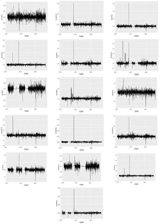
Figure 1.
The portfolio returns from 2010 to 2022 for small firms.
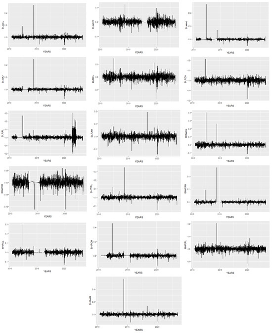
Figure 2.
The portfolio returns from 2010 to 2022 for big firms.
Table 1 summarizes the key statistics of thirty-two portfolios. Or findings reveal that among small portfolios, SHRAH exhibits the highest average return (0.0028) along with the highest standard deviation (0.0224). Furthermore, SHWAL reports the second-highest value among these groups following the highest value of standard deviation. Conversely, among these portfolios, SHRCL reports the lowest mean value of 0.0006 along with the lowest standard deviation value of 0.0152. Furthermore, among big portfolios, BHRAH reports the highest mean value along with the highest standard deviation value, while BLRCL reports the lowest mean and the highest value of standard deviation. These findings confirm that small stocks report a considerably higher mean value along with the standard deviation value as compared to big portfolios. Such findings are in line with the findings of Fama and French (1992, 1993, 2015), who documented that small stocks considerably earn higher returns than big stocks, along with the highest value of standard deviation.

Table 1.
Descriptive statistics of portfolios.
Table 2 shows the summary statistics of the risk factors. The market risk factor reports the highest mean value among other risk factors. Such findings indicate that market risk premiums yield higher returns along with the highest value of standard deviation. Furthermore, the labor income growth premium reports the second-highest mean value following the market risk premium. Additionally, this factor reports the lowest standard deviation value as compared to other risk factors. Moreover, size and investment premium report the third- and fourth-highest mean values among the group, along with standard deviation values. Conversely, value and profitability report a negative mean value as compared to other risk factors.
Table 2.
Descriptive statistics of risk factors.
Table 3 illustrates the correlations among the study variables, indicating that size, value, profitability, and investment premiums are negatively correlated with the market risk premium, whereas the human capital premium shows a positive correlation with the market risk premium. Additionally, all correlation coefficients are below 0.80, confirming the absence of multicollinearity concerns (Gujarati 2009).
Table 3.
Correlation matrix.
4.2. Fama and MacBeth (1973) Regression for Full Sample and COVID-19 Period
The Fama and MacBeth (1973) regression results presented in Table 4 indicate a significant positive effect of market premium (MKT) on the portfolio excess returns of small and big portfolios. The findings of the size premium (SMB) indicate that a small portfolio (SLWCL, SLWCH, SLWAL, SLWAH, and SLRCL) exhibits a significant and positive relationship with excess returns of small-stock portfolios. Contrastingly, some small portfolio reports (SLRCH) report positive and insignificant associations. Furthermore, for big portfolios, we find that the size premium exhibits a positive and statistically significant relationship with excess returns of large portfolios, except for BHWAH and BHRAL, where we find a positive and insignificant association. Conversely, we report that SMB has a significant and insignificant association with excess portfolio returns of big stocks (BHWCL, BHWCH, BHRCL, and BHRCH). For value premium, we report that HML demonstrates a significant positive association with excess portfolio returns of small stocks, except SLWAL and SLRAL, where we report a positive and insignificant association. Moreover, our findings report that the value premium demonstrates a significant positive association with excess portfolio returns of big stocks, except for BHWCL, BHWCH, and BHWAL, where we report positive and insignificant associations. Furthermore, we observe that the profitability premium exhibits a substantial positive and negative association with excess portfolio returns of small and big stocks. Additionally, we find that investment premium exhibits notable positive and negative influences on excess portfolio returns of small and big stocks, except for SHRAH, BLWAL, and BLRAL, where we report negative and insignificant associations. Lastly, for the human capital premium, we report that LBR is positively and significantly related to excess portfolio returns of small and big stocks, except for SHRCL, BLRCL, BHRCL, and BHRCH, where we report that LBR has a negative and insignificant impact on excess portfolio returns. Moreover, to validate the robustness of the main findings, we used a subsample analysis by dividing our data into during- and post-COVID-19 periods. This approach is methodologically justified and empirically supported in the recent literature that highlights the structural breaks and shifts in market dynamics caused by global crises (Hu 2022; Wei et al. 2023). Therefore, splitting the sample allows us to examine the temporal consistency of factor pricing and assess whether the model maintains its explanatory power under varying market conditions. Prior studies have shown that the COVID-19 pandemic introduced significant uncertainty and anomalies in financial markets, making such period-based analysis particularly useful for robustness checks (Maharani and Narsa 2023; Prasad et al. 2024).
Table 4.
Human capital six-factor model: full sample performance insights.
Table 5 presents the empirical findings of the model during the COVID-19 pandemic. The results indicate that the market premium (MKT) is positively and significantly related to excess portfolio returns of small and big portfolios, but the predictive power for explaining the association significantly decreased. More interestingly, we report that SMB exhibits a significant and positive association with the excess portfolio return of small stocks during COVID-19. Such findings indicate that size premiums are significantly priced in the Indian equity market during the COVID-19 pandemic. Conversely, in big stocks, we report positive, negative, and insignificant associations. Furthermore, we report that the performance of the value premium significantly improved during the COVID-19 pandemic compared to the full sample estimation. The results indicate that HML exhibits a significant, positive association with excess portfolio returns of small and big stocks. For profitability premium, we report positive, negative, and significant associations between RMW and excess portfolio returns of small and big stocks. Contrastingly, we observe that during COVID-19, investment premiums exhibited a significant negative influence on excess portfolio returns. Additionally, LBR shows a positive but statistically insignificant relationship with excess portfolio returns during the pandemic period. Lastly, in comparison to the predictive power of the augmented six-factor model, the performance of this model significantly decreased during the COVID-19 pandemic, as highlighted by the significant and insignificant association of risk factors with excess portfolio returns.
Table 5.
Human capital six-factor model: insights from the COVID-19 crisis period.
Table 6 illustrates the augmented six-factor model’s performance after the pandemic, showing that market premium (MKT) positively and significantly impacts excess returns in small and big portfolios. Such findings indicate that market risk premium is significantly priced in three sample conditions (full, during, and post-COVID-19). Conversely, the predictive power of SMB, HML, RMW, CMA, and LBR significantly decreased during this period.
Table 6.
Human capital six-factor model: insights from the post-pandemic era.
Table 7 presents a model comparison based on adjusted R2 (Adj-R2) values. Our findings demonstrate that risk factors substantially account for the variability in excess portfolio returns over the full sample. The augmented six-factor model exhibited a notable decline in predictive power during the COVID-19 pandemic relative to the entire sample period. More specifically, post-COVID-19 analysis showed a gradual improvement in the model’s efficiency in explaining time-series variability relative to the pandemic period.
Table 7.
Model comparison based on Adj-R2.
Table 8 presents the GRS and GRS-F test results, indicating partial rejection of the null hypothesis of portfolio efficiency in certain periods, suggesting that the models do not fully capture systematic risks. During the full sample period, the GRS statistics are relatively low, with the FF3FM being marginally significant. The mean absolute alpha values are also low, with the FF3FM and HC6FM models both showing the smallest value, indicating minimal mispricing and relatively efficient asset pricing throughout the sample period. However, during the COVID-19 period, the GRS statistics became more significant across all models, indicating a stronger rejection of portfolio efficiency during this crisis period. The mean absolute alpha values increase compared to the full sample, with the HC6FM and FF5FM both showing the smallest value. This suggests that although these models experienced increased mispricing during COVID-19, they were still relatively more efficient compared to the CAPM and FF3FM. In the post-COVID-19 period, the GRS statistics decreased slightly, indicating some improvement in model performance compared to the COVID-19 period. The HC6FM records the lowest GRS value, suggesting a relatively better performance among the models. Additionally, the mean absolute alpha value for HC6FM is the smallest, indicating that the human capital-based model has fewer pricing errors in the post-pandemic recovery period. Overall, the findings indicate that the HC6FM model generally performed better during both the COVID-19 and post-COVID-19 periods, as reflected by lower mean alpha values and GRS statistics. These results are consistent with Fama and French (2015), who noted that asset pricing models often face challenges in capturing systematic risks during turbulent periods, but the inclusion of human capital factors appears to improve pricing accuracy.
Table 8.
Comparison of competing asset pricing models (CAPM, FF3FM, FF5FM, and HC6FM) in a crisis period using the GRS test.
4.3. Rolling-Window Fama and MacBeth (1973) Regression
Table 9 reports the results of the rolling-window Fama and MacBeth (1973) two-pass regression. Factor loadings are estimated over a 36-month rolling-window that moves forward monthly, incorporating the subsequent month and dropping the earliest. The analysis reveals that the examined risk factors fail to adequately account for future portfolio return variations in the Indian equity market. More specifically, factor loadings show inconsistent statistical significance across portfolios in the two-pass regression. Therefore, associated risk premiums did not fully capture the variability in future returns. The model’s poor performance across portfolios implies that past betas are ineffective predictors. These outcomes concur with the findings of Khan and Afeef (2024) and Thalassinos et al. (2023) in emerging market contexts.
Table 9.
Rolling-window estimation of the Fama–Macbeth two-pass regression.
4.4. Discussion: Theoretical and Empirical Implications of the Study
The findings of this study align well with previous research. Consistent with the theoretical foundation laid by Markowitz (1952), a portfolio that maximizes returns while minimizing variance is considered efficient. In line with the CAPM framework, our findings reveal that the market premium significantly captures variability in portfolio returns. More specifically, our empirical findings reaffirm the central role of the market risk premium in explaining return variability across portfolios, consistent with foundational asset pricing theories, such as CAPM and its multifactor extensions. Moreover, the significant pricing of factors in the Indian market echoes the multifactor framework advocated by Fama and French (1992, 2015) and the emerging literature emphasizing the importance of human capital as a vital explanatory variable (Jagannathan and Wang 1996; Khan et al. 2023; Khan and Afeef 2024). Additionally, the Fama and French three-factor (FF3FM) and five-factor (FF5FM) models effectively capture risk exposures reflected in excess portfolio returns.
Similarly, Kolari et al. (2022) demonstrated that the ZCAPM outperforms traditional models, such as CAPM, FF3FM, and C4FM in explaining returns dispersion using global data. Liu (2023) documented that CAPM, FF3FM, and FF5FM significantly explain portfolio return variability during the COVID-19 pandemic. However, the observed decline in model performance during and after the COVID-19 pandemic aligns with recent findings that crisis periods introduce market anomalies and structural shifts that challenge traditional asset pricing frameworks (Hu 2022; Wei et al. 2023). Kausar et al. (2024), examining BRICS economies, found that firms with higher idiosyncratic risk (IR) experience lower returns compared to firms with lower IR. Our results corroborate the growing literature that identifies human capital, proxied by salaries and wages, as a significant factor in forecasting the time-series fluctuations of asset returns (Roy and Shijin 2018; Prasad et al. 2024). Furthermore, the superior explanatory power of the six-factor model during the full sample period supports prior studies suggesting that incorporating human capital enhances the model’s ability to capture asset return dynamics, especially in emerging economies with growing human capital potential (Maitai and Balakrishnan 2018; Maharani and Narsa 2023).
5. Conclusions
The MPT of Markowitz (1952, 1959) has attracted extensive scholarly attention in examining the risk–return relationship. Building on this foundation, the seminal works of Sharpe (1964) initiated the development of asset pricing models. Over the past decades, the CAPM has been widely used to explore the nuanced dynamics between risk and return. However, the restrictive assumptions of the CAPM have been challenged, leading researchers to propose multifactor models aimed at better explaining the variability in asset returns. Despite these advancements, such models often fall short of fully capturing asset return variations across different financial markets. Moreover, their performance and robustness during periods of economic and financial crises, geopolitical tensions, invasions, and pandemics have not been sufficiently explored. This study addresses existing research gaps by testing the HC6FM in the Indian equity market. Daily stock prices of Nifty-500 companies from July 2010 to June 2023, alongside yearly balance sheet data (2010–2022), were used to form 32 portfolios following the methodology of Fama and French (2015). The data were divided into full, COVID-19, and post-COVID periods to evaluate model robustness across different market phases. The Fama and MacBeth (1973) regression results highlight that the pandemic induced marked volatility, leading to many portfolios with inefficient returns and increased risk. Smaller portfolios generate superior returns but at the expense of higher risk relative to larger portfolios.
Our results confirm that, across all portfolios, the market premium plays a significant role in explaining return variability over time. In addition, size, value, profitability, investment, and human capital factors are significantly linked to excess portfolio returns, indicating these factors are meaningfully priced in the Indian market. The six-factor model demonstrates superior explanatory power during the full sample period compared to the pandemic and post-pandemic phases, with a marked reduction in model efficiency during and after the COVID-19 crisis. Importantly, our study extends the FF5FM by incorporating the human capital factor, operationalized as the labor income growth rate, which significantly prices the variability in asset returns. This finding suggests that investors should incorporate human capital considerations when conducting fundamental and technical analyses of Indian companies. Our results indicate that incorporating human capital, such as labor income growth, into asset pricing models greatly improves their explanatory power in emerging markets, like India. To enable this integration, labor data infrastructure and corporate reporting must be strengthened. During economic disruptions, models, like HC6FM, can offer deeper insights into market vulnerabilities.
Future research can extend the current study in several ways. First, future studies can test the performance of HC6FM in emerging and frontier markets to further enrich valuable insights into the model’s robustness and cross-market applicability. Second, the model could be enriched by incorporating additional risk factors that capture dimensions of investment behavior, such as Environmental, Social, and Governance (ESG) scores, geopolitical risk, and economic policy uncertainty. These additions may significantly enhance the model’s explanatory power, particularly during periods of heightened market volatility or systemic shocks. Third, future studies may benefit from employing more estimation techniques, like the generalized method of moments (GMM), instrumental variable (IV-GMM), and panel data models. Lastly, future studies could focus on firm-level analyses, investigating how human capital intensity interacts with firm characteristics to influence asset pricing. This would offer a more granular understanding of the economic mechanisms through which human capital contributes to expected returns.
Author Contributions
Conceptualization, N.K. and M.A.; methodology, N.K.; software, N.K.; validation, M.A., H.Z., and E.T.; formal analysis, N.K.; investigation, S.A.; resources, H.Z.; data curation, H.Z.; writing—original draft preparation, N.K.; writing—review and editing, E.T.; visualization, M.A.; supervision, H.Z.; project administration, S.A. All authors have read and agreed to the published version of the manuscript.
Funding
This research received no external funding.
Data Availability Statement
The raw data supporting the conclusions of this article will be made available by the authors on request.
Conflicts of Interest
The authors declare no conflicts of interest.
Abbreviations
The following abbreviations are used in this manuscript:
| CAPM | Capital asset pricing model |
| C4FM | Carhart four-factor model |
| FF3FM | Fama and French three-factor model |
| FF5FM | Fama and French five-factor model |
| FMB | Fama and MacBeth regression |
| P | Portfolio |
Appendix A
Table A1.
Variable computation and definition.
Table A1.
Variable computation and definition.
| Variable | Proxy | Computation | References |
|---|---|---|---|
| Market premium | MKT | RM-RF | Sharpe (1964) |
| Size premium | SMB | Market capitalization | Fama and French (1993) |
| Value premium | HML | Book value of equity/market value of equity | Fama and French (1993) |
| Profitability premium | RMW | EBIT/book value of equity | Fama and French (2015) |
| Investment premium | CMA | Growth in total assets | Fama and French (2015) |
| Human capital | LBR | Growth in salaries and wages | Roy and Shijin (2018), Khan et al. (2022), Thalassinos et al. (2023), Prasad et al. (2024) |
Note: In Table A1, the term RM refers to the market return and RF refers to the risk-free rate, which is equal to the expected rate of return of the market minus the risk-free rate of return.
Table A2.
Portfolio construction.
Table A2.
Portfolio construction.
| Sort | Breakpoints | Factor Constructions |
|---|---|---|
| Sort (2 × 2 × 2 × 2 × 2) the data on Size and book-to-market ratio, size and operating profitability Size and investment Size and human capital | Size: index median | SMBB/M = (SL + SH)/2 − (BL + BH)/2 SMBOp = (SR + SW)/2 − (BR + BW)/2 SMBInv = (SC + SA)/2 − (BC + BA)/2 SMBLbr = (SLhr + SHhr)/2 − (BLhtr + BHhr)/2 |
Construction of Factor Premiums:
Table A3.
Portfolio labels and abbreviations.
Table A3.
Portfolio labels and abbreviations.
| Label | Abbreviations |
| SLWCL | Small firms with low B/M, weak profitability, conservative investment, and low labor income growth |
| SLWCH | Small firms with low B/M, weak profitability, conservative investment, and high labor income growth |
| SLWAL | Small firms with low B/M, weak profitability, aggressive investment, and low labor income growth |
| SLWAH | Small firms with low B/M, weak profitability, aggressive investment, and high labor income growth |
| SLRCL | Small firms with low B/M, robust profitability, conservative investment, and low labor income growth |
| SLRCH | Small firms with low B/M, robust profitability, conservative investment, and high labor income growth |
| SLRAL | Small firms with low B/M, robust profitability, aggressive investment, and low labor income growth |
| SLRAH | Small firms with low B/M, robust profitability, aggressive investment, and high labor income growth |
| SHWCL | Small firms with high B/M, weak profitability, conservative investment, and low labor income growth |
| SHWCH | Small firms with high B/M, weak profitability, conservative investment, and high labor income growth |
| SHWAL | Small firms with high B/M, weak profitability, aggressive investment, and low labor income growth |
| SHWAH | Small firms with high B/M, weak profitability, aggressive investment, and high labor income growth |
| SHRCL | Small firms with high B/M, robust profitability, conservative investment, and low labor income growth |
| SHRCH | Small firms with high B/M, robust profitability, conservative investment, and high labor income growth |
| SHRAL | Small firms with high B/M, robust profitability, aggressive investment, and low labor income growth |
| SHRAH | Small firms with high B/M, robust profitability, aggressive investment, and high labor income growth |
| BLWCL | Big firms with low B/M, weak profitability, conservative investment, and low labor income growth |
| BLWCH | Big firms with low B/M, weak profitability, conservative investment, and high labor income growth |
| BLWAL | Big firms with low B/M, weak profitability, aggressive investment, and low labor income growth |
| BLWAH | Big firms with low B/M, weak profitability, aggressive investment, and high labor income growth |
| BLRCL | Big firms with low B/M, robust profitability, conservative investment, and low labor income growth |
| BLRCH | Big firms with low B/M, robust profitability, conservative investment, and high labor income growth |
| BLRAL | Big firms with low B/M, robust profitability, aggressive investment, and low labor income growth |
| BLRAH | Big firms with low B/M, robust profitability, aggressive investment, and high labor income growth |
| BHWCL | Big firms with high B/M, weak profitability, conservative investment, and low labor income growth |
| BHWCH | Big firms with high B/M, weak profitability, conservative investment, and high labor income growth |
| BHWAL | Big firms with high B/M, weak profitability, aggressive investment, and low labor income growth |
| BHWAH | Big firms with high B/M, weak profitability, aggressive investment, and high labor income growth |
| BHRCL | Big firms with high B/M, robust profitability, conservative investment, and low labor income growth |
| BHRCH | Big firms with high B/M, robust profitability, conservative investment, and high labor income growth |
| BHRAL | Big firms with high B/M, robust profitability, aggressive investment, and low labor income growth |
| BHRAH | Big firms with high B/M, robust profitability, aggressive investment, and high labor income growth |
Notes
| 1 | |
| 2 |
References
- Amar, Syamsul, and Ikbar Pratama. 2020. Exploring the link between income inequality, poverty reduction and economic growth: An ASEAN perspective. International Journal of Innovation, Creativity and Change 11: 24–41. [Google Scholar]
- Anuno, Fernando, Mara Madaleno, and Elisabete Vieira. 2023. Using the capital asset pricing model and the Fama–French Three-Factor and Five-Factor models to manage stock and bond portfolios: Evidence from Timor-Leste. Journal of Risk and Financial Management 16: 480. [Google Scholar]
- Baker, Scott R., Nicholas Bloom, Steven J. Davis, Kyle J. Kost, Marco C. Sammon, and Tasaneeya Viratyosin. 2020. The Unprecedented Stock Market Impact of COVID-19. No. w26945. National Bureau of Economic Research. Available online: https://www.nber.org/papers/w26945 (accessed on 17 June 2021).
- Banz, Rolf W. 1981. The relationship between return and market value of common stocks. Journal of Financial Economics 9: 3–18. [Google Scholar] [CrossRef]
- Barras, Laurent. 2019. A large-scale approach for evaluating asset pricing models. Journal of Financial Economics 134: 549–69. [Google Scholar] [CrossRef]
- Basu, Sanjoy. 1977. Investment performance of common stocks in relation to their price-earnings ratios: A test of the efficient market hypothesis. The Journal of Finance 32: 663–82. [Google Scholar]
- Basu, Sanjoy. 1983. The relationship between earnings yield, market value and return for NYSE common stocks. Journal of Financial Economics 12: 129–56. [Google Scholar] [CrossRef]
- Bekaert, Geert, and Campbell R. Harvey. 2000. Foreign speculators and emerging equity markets. The Journal of Finance 55: 565–613. [Google Scholar] [CrossRef]
- Bekaert, Geert, and Campbell R. Harvey. 2003. Emerging markets finance. Journal of Empirical Finance 10: 3–55. [Google Scholar] [CrossRef]
- Belo, Frederico, Jun Li, Xiaoji Lin, and Xiaofei Zhao. 2017. Labor-force heterogeneity and asset prices: The importance of skilled labor. The Review of Financial Studies 30: 3669–709. [Google Scholar] [CrossRef]
- Bhandari, Laxmi Chand. 1988. Debt/equity ratio and expected common stock returns: Empirical evidence. The Journal of Finance 43: 507–28. [Google Scholar] [CrossRef]
- Black, Fischer, Michael C. Jensen, and Myron Scholes. 1972. The Capital Asset Pricing Model: Some Empirical Findings. In Studies in the Theory of Capital Markets. Edited by Jensen Michael. New York: Praeger Publishers, pp. 79–124. [Google Scholar]
- Breeden, Douglas T. 1979. An intertemporal asset pricing model with stochastic consumption and investment opportunities. Journal of Financial Economics 7: 265–96. [Google Scholar] [CrossRef]
- Brown, Stephen J., William Goetzmann, Roger G. Ibbotson, and Stephen A. Ross. 1992. Survivor-ship bias in performance studies. Review of Financial Studies 5: 553–80. [Google Scholar] [CrossRef]
- Campbell, John Y. 1996. Understanding risk and return. Journal of Political Economy 104: 298–345. [Google Scholar] [CrossRef]
- Carhart, Mark M. 1997. On persistance in mutual fund performance. The Journal of Finance LII: 57–82. [Google Scholar]
- Chittedi, Krishna Reddy. 2015. Global stock markets development and integration: With special reference to BRIC countries. IUP Journal of Applied Economics 14: 5–20. [Google Scholar]
- Cochrane, John H. 1996. A Cross-Sectional Test of an Investment-Based Asset Pricing Model. Journal of Political Economy 104: 572–621. [Google Scholar] [CrossRef]
- Connor, Gregory, and Robert Korajczyk. 1989. An intertemporal equilibrium beta pricing model. The Review of Financial Studies 2: 373–92. [Google Scholar] [CrossRef]
- Contessi, Silvio, and Pierangelo De Pace. 2021. The international spread of COVID-19 stock market collapses. Finance Research Letters 42: 101894. [Google Scholar] [CrossRef]
- Cox, John C., Jonathan E. Ingersoll, and Stephen A. Ross. 1985. An intertemporal general equilibrium model of asset prices. Econometrica 53: 385–408. [Google Scholar] [CrossRef]
- Diebolt, Claude, and Ralph Hippe. 2019. The long-run impact of human capital on innovation and economic development in the regions of Europe. Applied Economics 51: 542–63. [Google Scholar] [CrossRef]
- Elton, Edwin J., Martin J. Gruber, and Christopher R. Blake. 1996a. Survivorship bias and mutual fund performance. The Review of Financial Studies 9: 1097–120. [Google Scholar] [CrossRef]
- Elton, Edwin J., Martin J. Gruber, Sanjiv Das, and Christopher R. Blake. 1996b. The persistence of risk-adjusted mutual fund performance. Journal of Business 69: 133–57. [Google Scholar] [CrossRef]
- Elton, Edwin J., Martin J. Gruber, Sanjiv Das, and Matthew Hlavka. 1993. Efficiency with costly information: A re-interpretation of evidence from managed portfolios. Review of Financial Studies 6: 1–21. [Google Scholar] [CrossRef]
- Eun, Cheol, Kyuseok Lee, and Fengrong Wei. 2023. Dual role of the country factors in international asset pricing: The local factors and proxies for the global factors. International Review of Financial Analysis 89: 102760. [Google Scholar] [CrossRef]
- Fama, Eugene F. 1970. Efficient Capital Markets: A review of theory and empirical work. The Journal of Finance 25: 383–417. [Google Scholar] [CrossRef]
- Fama, Eugene F., and James D. MacBeth. 1973. Risk, return and equilibrium: Empirical Tests. The Journal of Political Economy 81: 607–36. [Google Scholar] [CrossRef]
- Fama, Eugene F., and Kenneth R. French. 1992. The cross-section of expected stock returns. The Journal of Finance 47: 427–65. [Google Scholar]
- Fama, Eugene F., and Kenneth R. French. 1993. Common risk factors in the returns on stocks and bonds. Journal of Financial Economics 33: 3–56. [Google Scholar] [CrossRef]
- Fama, Eugene F., and Kenneth R. French. 2015. A five factor asset pricing model. Journal of Financial Economics 116: 1–22. [Google Scholar] [CrossRef]
- Fama, Eugene F., and Kenneth R. French. 2018. Choosing factors. Journal of Financial Economics 128: 234–52. [Google Scholar] [CrossRef]
- Fisher, Irving. 1907. The Rate of Interest. In History of Economic Thought Books from McMaster University Archive for the History of Economic Thought. Hamilton: McMaster University. [Google Scholar]
- Friend, Irwin, Randolph Westerfield, and Michael Granito. 1978. New evidence on the capital asset pricing model. The Journal of Finance 33: 903–17. [Google Scholar] [CrossRef]
- Gao, Meng. 2023. Tests of the Fama-French five-factor model in the US stock market under the COVID-19 pandemic. Paper presented at 2023 2nd International Conference on Economics, Smart Finance and Contemporary Trade (ESFCT 2023), Dali, China, July 28–30. [Google Scholar]
- Gibbons, Michael R., Stephen A. Ross, and Jay Shanken. 1989. A test of the efficiency of a given portfolio. Econometrica 57: 1121. [Google Scholar] [CrossRef]
- Goetzmann, William N., and Roger Ibbotson. 1994. Do winners repeat? Patterns in mutual fund performance. Journal of Portfolio Management 20: 9–18. [Google Scholar]
- Gujarati, Damodar N. 2009. Basic Econometrics. New Delhi: Tata McGraw-Hill Education. [Google Scholar]
- Haroon, Omair, and Syed Aun R. Rizvi. 2020. COVID-19: Media coverage and financial markets behavior a sectoral inquiry. Journal of Behavioral and Experimental Finance 27: 100343. [Google Scholar] [CrossRef]
- Harshita, Singh, and Surendra S. Yadav. 2015. Indian stock market and the asset pricing models. Procedia Economics and Finance 30: 294–304. [Google Scholar] [CrossRef]
- Harvey, Campbell R., Yan Liu, and Heqing Zhu. 2016. …and the cross-section of expected returns. Review of Financial Studies 29: 5–68. [Google Scholar] [CrossRef]
- He, Pinglin, Yulong Sun, Ying Zhang, and Tao Li. 2020. COVID-19’s Impact on Stock Prices across Different Sectors—An Event Study Based on the Chinese Stock Market. Emerging Markets Finance and Trade 56: 2198–212. [Google Scholar] [CrossRef]
- Hendricks, Darrayll, Jayendu Patel, and Richard Zeckhauser. 1993. Hot hands in mutual funds: Short-run persistence of performance, 1974–88. Journal of Finance 48: 93–130. [Google Scholar]
- Hou, Kewei, Chen Xue, and Lu Zhang. 2020. Replicating anomalies. Review of Financial Studies 33: 2019–133. [Google Scholar] [CrossRef]
- Hu, Tianmu. 2022. A Study on the Influence of the COVID-19 Epidemic on American Stock Market Based on the Fama-French Five-Factor Model. In Proceedings of the International Conference on Business and Policy Studies, Stamford, CA, USA, 12 March 2022. Singapore: Springer Nature Singapore, pp. 870–84. [Google Scholar]
- Jagannathan, Ravi, and Zhenyu Wang. 1996. The conditional CAPM and the cross-section of expected returns. The Journal of Finance 51: 3–53. [Google Scholar]
- Jagannathan, Ravi, Keiichi Kubota, and Hitoshi Takehara. 1998. Relationship between labor-income risk and average return: Empirical evidence from the Japanese stock market. Journal of Business 71: 319–47. [Google Scholar] [CrossRef]
- Jegadeesh, Narasimhan, and Sheridan Titman. 1993. Returns to buying winners and selling losers: Implications for stock market efficiency. Journal of Finance 48: 65–91. [Google Scholar] [CrossRef]
- Kan, Raymond, Xiaolu Wang, and Xinghua Zheng. 2024. In-sample and out-of-sample Sharpe ratios of multi-factor asset pricing models. Journal of Financial Economics 155: 103837. [Google Scholar] [CrossRef]
- Kausar, Saba, Syed Zulfiqar Ali Shah, and Abdul Rashid. 2024. Determinants of idiosyncratic risk: Evidence from BRICS countries. Asia-Pacific Journal of Business Administration 16: 553–74. [Google Scholar] [CrossRef]
- Khan, Naveed, and Mustafa Afeef. 2024. Is human capital premium price in asset pricing? Insights from South Africa during the COVID-19 era. Journal of Innovative Research in Management Sciences 5: 1–24. [Google Scholar] [CrossRef]
- Khan, Naveed, Hassan Zada, and Imran Yousaf. 2022. Does premium exist in the stock market for labor income growth rate? A six-factor-asset-pricing model: Evidence from Pakistan. Annals of Financial Economics 17: 2250017. [Google Scholar] [CrossRef]
- Khan, Naveed, Hassan Zada, Shakeel Ahmed, Fayaz Ali Shah, and Shahid Jan. 2023. Human capital-based four-factor asset pricing model: An empirical study from Pakistan. Heliyon 9: e16328. [Google Scholar] [CrossRef] [PubMed]
- Khan, Naveed, Mustafa Afeef, and Hassan Zada. 2025. Human capital in asset pricing: The case of the Brazilian stock market during crisis periods. Modern Finance 3: 29–57. [Google Scholar] [CrossRef]
- Kim, Dongcheol, Tong Suk Kim, and Byoung-Kyu Min. 2011. Future labor income growth and the cross-section of equity returns. Journal of Banking & Finance 35: 67–81. [Google Scholar]
- Kolari, James W., Jianhua Z. Huang, Hilal Anwar Butt, and Huiling Liao. 2022. International tests of the ZCAPM asset pricing model. Journal of International Financial Markets, Institutions and Money 79: 101607. [Google Scholar] [CrossRef]
- Kuehn, Lars-Alexander, Mikhail Simutin, and Jessie Jiaxu Wang. 2017. A labor capital asset pricing model. The Journal of Finance 72: 2131–78. [Google Scholar] [CrossRef]
- Lettau, Martin, Sydney C Ludvigson, and Sai Ma. 2019. Capital share risk in U.S. asset pricing. The Journal of Finance 74: 1753–92. [Google Scholar] [CrossRef]
- Levy, Hain. 1983. The capital asset pricing model: Theory and empiricism. The Economic Journal 93: 145–65. [Google Scholar] [CrossRef]
- Linnainmaa, Juhani T., and Michael R. Roberts. 2018. The history of the cross-section of stock returns. Review of Financial Studies 31: 2606–49. [Google Scholar] [CrossRef]
- Lintner, John. 1965. Security prices, risk, and maximal gains from diversification. The Journal of Finance 20: 587–615. [Google Scholar]
- Liu, Haiyue, Aqsa Manzoor, CangYu Wang, Lei Zhang, and Zaira Manzoor. 2020a. El brote de COVID-19 y la respuesta del mercado de valores de los países afectados. Revista Internacional de Investigación Ambiental y Salud Pública 17: 2800. [Google Scholar]
- Liu, Yuxuan. 2023. A Comparison of Three Asset-pricing Models During COVID-19. Highlights in Business, Economics and Management 7, 144–49. [Google Scholar]
- Lucas, Rober E. 1978. Asset Prices in an exchange economy. Econometrica 46: 1429–45. [Google Scholar] [CrossRef]
- Lustig, Hanno, Stijin Van Nieuwerburgh, and Adrien Verdelhan. 2013. The wealth-consumption ratio. The Review of Asset Pricing Studies 3: 38–94. [Google Scholar] [CrossRef]
- Maharani, Astrid, and Made Narsa. 2023. Six-factor plus intellectual capital in the capital asset pricing model and excess stock return: Empirical evidence in emerging stock markets. Cogent Economics & Finance 11: 2252652. [Google Scholar]
- Maitai, Moinak, and A. Balakrishnan. 2018. Is human capital the six factor. Journal of Economic Studies 45: 710–37. [Google Scholar] [CrossRef]
- Maiti, Moinak, and Darko Vukovic. 2020. Role of human capital assets in measuring firm performance and its implication for firm valuation. Journal of Economic Structures 9: 1–27. [Google Scholar] [CrossRef]
- Markowitz, Harry. 1952. Portfolio selection. The Journal of Finance 7: 77–91. [Google Scholar]
- Markowitz, Harry. 1959. Portfolio Selection: Efficient diversification of Investments. New York: Wiley. [Google Scholar]
- Mayers, David. 1972. Nonmarketable assets and capital market equilibrium under uncertainty. In Studies in the Theory of Capital Markets. Edited by Michael C. Jensen. New York: Praeger, pp. 223–48. [Google Scholar]
- Miller, Merton H., and Franco Modigliani. 1961. Dividend Policy, Growth, and the Valuation of Shares. The Journal of Business 34: 411–33. [Google Scholar] [CrossRef]
- Mishra, Harshit, and Parama Barai. 2024. Entropy Augmented Asset Pricing Model: Study on Indian Stock Market. Asia-Pacific Financial Markets 31: 81–99. [Google Scholar] [CrossRef]
- Mohanasundaram, S., and R. Kasilingam. 2024. The sustainability factor in asset pricing: Empirical evidence from the Indian market. Quarterly Review of Economics and Finance 94: 206–13. [Google Scholar] [CrossRef]
- Mossin, Jan. 1966. Equilibrium in a Capital Asset Market. Econometrica 34: 768–83. [Google Scholar] [CrossRef]
- Mzoughi, Hela, Christian Urom, Gazi Salah Uddin, and Khaled Guesmi. 2020. The Effects of COVID-19 Pandemic on Oil Prices, CO2 Emissions and the Stock Market: Evidence from a Var Model. Available online: https://papers.ssrn.com/sol3/papers.cfm?abstract_id=3587906 (accessed on 19 May 2020).
- National Stock Exchange of India (NSE). 2022. Market Capitalisation Report. Available online: https://www.nseindia.com (accessed on 17 June 2021).
- Onali, Enroci. 2020. COVID-19 and Stock Market Volatility. Available online: https://papers.ssrn.com/sol3/papers.cfm?abstract_id=3571453 (accessed on 28 May 2020).
- Papp, Bela. 2022. Which Factors in BRICS? Available online: https://jyx.jyu.fi/jyx/Record/jyx_123456789_80794 (accessed on 4 April 2022).
- Park, Dojoon, Young Ho Eom, and Jaehoon Hahn. 2021. Evaluating the conditional CAPM using consumption-based state variables: Evidence from the Korean stock market. Korean Journal of Financial Studies 50: 339–67. [Google Scholar] [CrossRef]
- Prasad, Saroj S., Ashutosh Verma, Priti Bakhshi, and Shantanu Prasad. 2024. Superiority of six factor model in Indian stock market. Cogent Economics and Finance 12: 2411567. [Google Scholar] [CrossRef]
- Qin, Jie. 2002. Human-capital-adjusted capital asset pricing model. The Japanese Economic Review 53: 182–98. [Google Scholar] [CrossRef]
- Reuters. 2020. La Oficina de Estadísticas de Italia Pronostica que el PIB Caerá un 8,3% en 2020 por el Impacto del Coronavirus. Available online: https://www.swissinfo.ch/spa/italia-prev%C3%A9-una-ca%C3%ADda-del-8-3-del-pib-en-2020/45822862 (accessed on 8 June 2020).
- Roll, Roll. 1977. A critique of the asset pricing theory’s tests part I: On past and potential testability of the theory. Journal of Financial Economics 4: 129–76. [Google Scholar] [CrossRef]
- Romer, Paul M. 1990. Human capital and growth: Theory and evidence. Carnegie-Rochester Conference Series on Public Policy 32: 251–28. [Google Scholar] [CrossRef]
- Rosenberg, Barr, Kenneth Reid, and Ronald Lanstein. 1985. Persuasive evidence of market inefficiency. The Journal of Portfolio Management 11: 9–16. [Google Scholar] [CrossRef]
- Ross, Stephen A. 1976. The arbitrage theory of capital asset pricing. Journal of Economic Theory 13: 341–60. [Google Scholar] [CrossRef]
- Ross, Stephen A. 1978. The current status of the capital asset pricing model (CAPM). The Journal of Finance 33: 885–901. [Google Scholar] [CrossRef]
- Roy, Rahul, and Santhakumar Shijin. 2018. A six-factor asset pricing model. Borsa Istanbul Review 18: 205–17. [Google Scholar] [CrossRef]
- Roy, Rahul, and Santhakumar Shijin. 2019. Is human capital the sixth factor? Evidence from US data. ACRN Journal of Finance and Risk Perspectives 8: 21–55. [Google Scholar] [CrossRef]
- Samuelson, Paul A. 1969. Lifetime portfolio selection by dynamic stochastic programming. The Review of Economics and Statistics 51: 239–46. [Google Scholar] [CrossRef]
- Securities and Exchange Board of India (SEBI). 2023. Annual Report 2022–2023. Available online: https://www.sebi.gov.in (accessed on 6 March 2023).
- Setiawan, Budi, Adil Saleem, Robert Jeyakumar Nathan, Zoltan Zeman, Robert Magda, and Judit Barczi. 2021. Financial market development and economic growth: Evidence from ASEAN and CEE region. Polish Journal of Management Studies 23: 481–94. [Google Scholar] [CrossRef]
- Setiawan, Budi, Wikurendra Afin Rifai, Nathan Edza Aria, Robert Jeyakumar, and Maria Fekete-Farkas. 2022. COVID-19 pandemic, asset prices, risks, and their convergence: A survey of Islamic and G7 stock market, and alternative assets. Borsa Istanbul Review 22: 47–59. [Google Scholar] [CrossRef]
- Sharpe, William F. 1964. Capital asset prices: A theory of market equilibrium under conditions of risk. The Journal of Finance 19: 425–42. [Google Scholar]
- Shegal, Sanjay, Vibhuti Vasishth, and Florent Deisting. 2024. Lottery factor and stock returns: Evidence from India. Borsa Istanbul Review 24: 449–59. [Google Scholar] [CrossRef]
- Shijin, Santhakumar, Arun Kumar Gopalaswamy, and Debashis Acharya. 2012. Dynamic risk-return relation with human capital: A study on Indian markets. International Journal of Emerging Markets 7: 146–59. [Google Scholar] [CrossRef]
- Singh, Manish Kumar, and Yadawananda Neog. 2020. Efecto de contagio del brote de COVID-19: Otra receta para el desastre en la economía india. Revista de Asuntos Públicos 20: 1–8. [Google Scholar] [CrossRef]
- Son, Bumho, and Jaewook Lee. 2022. Graph-based multi-factor asset pricing model. Finance Research Letters 44: 102032. [Google Scholar] [CrossRef]
- Tambosi Filho, Elmo, Almir Martins Vieria, and Fabio Gallo Garcia. 2022. Testing conditional CAPM with the inclusion of human capital. Academy of Accounting and Financial Studies Journal 26: 1–08. [Google Scholar]
- Thalassinos, Eleftherios, Naveed Khan, Shakeel Ahmed, Hassan Zada, and Anjum Ihsan. 2023. A Comparison of Competing Asset Pricing Models: Empirical Evidence from Pakistan. Risks 11: 65. [Google Scholar] [CrossRef]
- Tobin, James. 1958. Liquidity Preference as Behavior towards Risk. The Review of Economic Studies 25: 65–86. [Google Scholar] [CrossRef]
- Tridico, Pasquale. 2007. The Determinants of Economic Growth in Emerging Economies: A Comparative Analysis. Roma: University Roma Tre. [Google Scholar]
- Vianna, Andre C., and Aandre V. Mollick. 2018. Institutions: Key variable for economic development in Latin America. Journal of Economics and Business 96: 42–58. [Google Scholar] [CrossRef]
- Wang, Shi-Xiao, Wen-Min Lu, and Shiu-Wan Hung. 2020. Improving innovation performance of emerging economies: The role of manufacturing. Managerial and Decision Economics 41: 503–19. [Google Scholar] [CrossRef]
- Wei, Jianing, Nanyi Xiao, and Luyue Zhang. 2023. Comparison of the performances for CAPM and Fama-French models during COVID-19. Paper presented at Third International Conference on Artificial Intelligence and Computer Engineering (ICAICE 2022), 126104R, Wuhan, China, April 28. [Google Scholar] [CrossRef]
- Wermers, Russ. 1996. Momentum Investment Strategies of Mutual Funds, Performance Persistence, and Survivorship Bias. Working Paper. Boulder: Graduate School of Business and Administration, University of Colorado at Boulder. [Google Scholar]
- World Bank. 2023. Global Economic Prospects. Available online: https://www.worldbank.org (accessed on 6 June 2023).
- Yilmazkuday, Hakan. 2021. COVID-19 effects on the S&P 500 index. Applied Economics Letters 1: 7–13. [Google Scholar] [CrossRef]
- Zada, Hassan, Mobeen Ur Rehman, and Muddasar Khwaja Ghani Khwaja. 2018. Application of Fama and French five factor model of asset pricing: Evidence from Pakistan stock market. International Journal of Economics, Management and Accounting 26: 1–23. [Google Scholar]
- Zaremba, Adam, Renatas Kizys, David Y. Aharon, and Ender Demir. 2020. Infected markets: Novel coronavirus, government interventions, and stock return volatility around the globe. Finance Research Letters 35: 101597. [Google Scholar] [CrossRef]


Disclaimer/Publisher’s Note: The statements, opinions and data contained in all publications are solely those of the individual author(s) and contributor(s) and not of MDPI and/or the editor(s). MDPI and/or the editor(s) disclaim responsibility for any injury to people or property resulting from any ideas, methods, instructions or products referred to in the content. |
© 2025 by the authors. Licensee MDPI, Basel, Switzerland. This article is an open access article distributed under the terms and conditions of the Creative Commons Attribution (CC BY) license (https://creativecommons.org/licenses/by/4.0/).