COVID-19 Intensity, Resilience, and Expected Returns

Abstract

This paper provides a model to interpret the relative behavior of expected returns of high- and low-resilience assets from the time of the COVID-19 pandemic, including a novel definition of disaster based on COVID-19 intensity. The setup allows us to disentangle the probability of disaster and investors’ updating probability at each point in time which sheds light on how long-memory investors react to disaster risk and play a role in future prices. The theoretical results show higher revisions in expected return differentials in the case of any perception of a higher possibility of disaster or, equivalently, higher COVID-19 intensity. The intensity of COVID-19 can directly exacerbate the heterogeneity in expected returns for high- and low-resilience assets and their corresponding differentials. More importantly, an increase in COVID-19 intensity increases the expected returns of low-resilience assets more than those of high-resilience ones.

1. Introduction

Disasters impose a huge amount of uncertainty on the stock market. They are usually identified by the intensity and probability of occurrence, which are practically unknown to investors and can create severe changes in stock prices (see Giglio et al. (2021); Hanspal et al. (2021); Gormsen and Koijen (2020)). Even the gradual unfolding of disaster realization can lead to a huge amount of heterogeneity in the harsh time of a crisis. This heterogeneity tightly depends on the type of disaster and the corresponding firm’s characteristics that make investors learn and update their beliefs.

Apart from uncertainty usually caused by any crisis, the COVID-19 pandemic induced a sort of heterogeneity directly related to specific firms’ characteristics. Some firms relative to others are less risky and more “resilient” to COVID-19-like pandemics, in the sense that these firms have more flexible workforces in the presence of social distancing rules and lockdown restrictions. Such flexibility empowers them to deal with corresponding managerial issues. In order to maximize shareholder wealth, firms need to diagnose and take different types of risk seriously in their decisions. In the post-pandemic era, “resilience” risk, which is directly related to the working environment, can be introduced as known risks and should be assessed and managed to optimize shareholder wealth. For risk management to affect value as Stulz (2024) explains, there should be a significant effect of risk on future expected cash flows. Daadmehr (2024) provides different pieces of evidence of heterogeneous expected cash flows and its impact on implied discount rates in the time of COVID-19. The COVID-19 literature provides different interpretations of how such risks can potentially affect expected returns (Pagano et al. 2023). Having evidence of the significant impact of COVID-19 on overall economic contraction (Daadmehr 2022) enables this paper to propose a novel specific asset pricing model considering a clear “definition” for COVID-19 disaster states to explain more precisely existing heterogeneity.

On the other hand, investors learn from not only the possibility of disaster that itself depends on COVID-19 intensity but also the duration of disaster. Yet, there is no study to show how such workplace-related risk can be transmitted from cash flows to expected returns, including the impact of COVID-19 disaster probability and investors’ updating probabilities as two different kinds of probabilities (opposed to Pagano et al. (2023)). 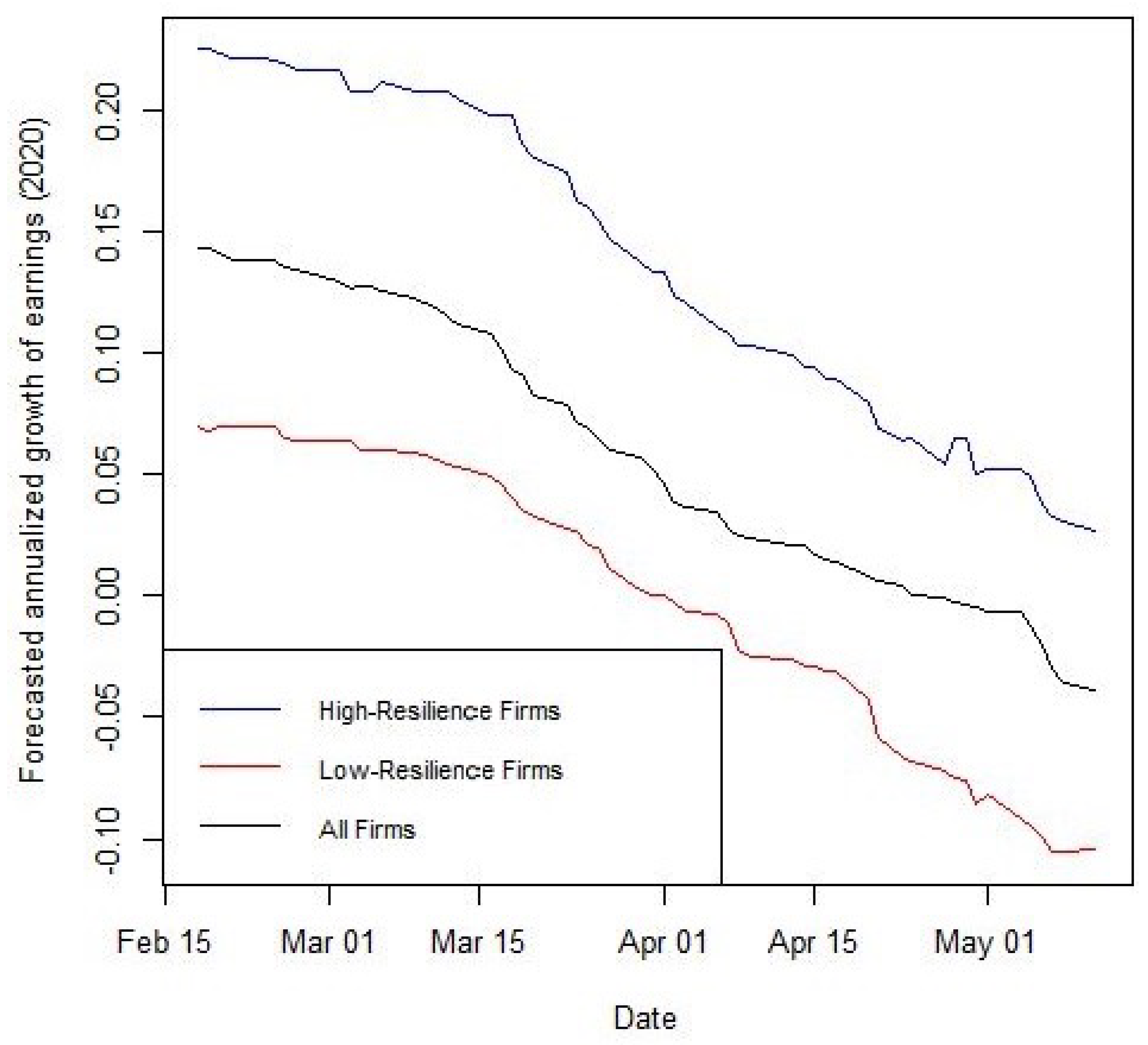As a piece of evidence, Figure 1 exhibits the lower growth of earning expectations for low-resilience firms. This figure suggests that workplace resilience can mitigate the consequences of the association between COVID-19 intensity and social distancing rules, which accelerates investors’ learning in favor of more workplace-flexible firms and updating trading strategies as well.

This paper tries to figure out what happened to expectations during the COVID-19 disaster when workplace flexibility was triggered by COVID-19 intensity. Improving the pricing methodology in Daadmehr (2024) to see the impact of the time-varying intensity of the disaster, this paper proposes a new setup and shows how the resilience and intensity of the COVID-19 pandemic interact with each other to establish the corresponding heterogeneity in expected returns. It explains the transit channel and proves the existence of heterogeneity in asset prices, expected returns, and its differentials, specifically due to not only workplace resilience but also COVID-19 intensity and the probability of disaster. Results emphasize the necessity and importance of disentangling investors’ updatingprobabilities and disaster probabilities and suggest that low-resilience firmshave higher expected returns than high-resilience ones, in line with Pagano et al. (2023) and Daadmehr (2024). Moreover, the model sheds light on investors’ learning originating from the intensity of COVID-19 and reveals to what extent expected returnsdepend on this novel insight which exhibits the lower bound for investors’ updating probabilities, based on the firm’s resilience as well as disaster probability and COVID-19 intensity. Results suggest fewer expected returns for more resilient assets and higher expected return differentials in cases of higher COVID-19 intensity, through investors’ learning.

In brief, this paper, as a novel work, provides theoretical proof and rationalizes empirical evidence in the literature. First, it defines “disaster periods” based on the intrinsic feature of this crisis and COVID-19 as an exogenous pathological disease. Second, it takes into account the fact that investors learn from the probability of disaster and update this probability to a new probability called investors’ updating probability (IUP), which depends on the duration of a crisis. Specifically, it shows analytically that an increase in COVID-19 intensity increases the expected returns of low-resilience assets more than those of high-resilience ones.

To this aim, after a quick review of the literature in Section 2, this paper explains the setup and provides results and solutions in Section 3 and Section 4, respectively; then, it concludes.

2. Motivation and Contribution to the Literature

From one side, this paper joins the literature in corporate resilience. This strand of the literature has grown fast, especially since COVID-19’s emergence. A wide range of studies deviate from the general definition of resilience as the capacity of firms to have a short recovery period in cases of any disturbance during and after a crisis. The definition of resilience in the period of COVID-19 is mostly accompanied by investigating the role of the working environment to create tolerance toward social distancing rules and lockdown restrictions in response to the exogenous COVID-19 pandemic. Apart from the early literature from 2020 that explains to what extent jobs can be carried out from home and the impact of this together with flexibility in on-site teamwork communication on firms’ production costs (see Koren and Pető (2020); Dingel and Neiman (2020); Hensvik et al. (2020)), some papers start to quantify corporate resilience based on firms’ financial status and interaction withworkplace flexibility which are main resilience-related characteristics (Daadmehr 2024). Although such studies provide key tools for risk management, there is still a long path to realize how different firms’ characteristics generate risk and expected return differentiation.

To do this, one may be interested in proposing an asset pricing setup in which the role of interaction between workplace resilience and cash flow sheds light on differentiation in expected returns. This paper contributes to studies in risk management from an asset pricing perspective, specifically when the economy is hit by rare events like the COVID-19 pandemic.

In the asset pricing literature, “rare disaster” appears as a response to the equity premium puzzle (see Campbell (2017) and Rietz (1988)) where preferences make expected returns greater than what consumption (distribution) implies. The early studies on rare disasters (Weitzman (2005); Rietz (1988); Barro (2006)) suggest that not only uncertainty but also a small possibility of disaster may lead to non-lognormality in consumption growth and its distribution tends to have a heavier tail (Weitzman 2005). Martin (2013) starts with power utility and arbitrary iid consumption growth and explains the role of the cumulant generating function for consumption risk. The proposed equity premium based on the generating function reveals an increasing trend in terms of relative risk aversion, meaning that a decreasing amount of RRA is needed to fit any given equity premium (Martin 2013).

There are two main strands in the literature in asset pricing with rare events. In the first strand, papers start to establish the importance of the state of the economy and take into account disaster probability in the sense of the probability of adverse events (see Barro (2006) and Daadmehr (2022)). Barro (2006) calibrated the probability of disaster based on historical data, including different kinds of rare events since WW1. A new asset pricing model for the COVID-19 period, including the macro-time effect of disasters on firms’ productivity as well as the price of an equity claim to the output of firms, is provided by Daadmehr (2022). The second strand starts to consider the sequence of disasters as a realization of the Poisson processes. Among all, Wachter and Zhu (2024) consider the aggregate consumption process containing the Poisson term for capturing the impact of disasters. They define disaster states based on two high and low amounts of intensity in the Poisson process and provide the theoretical evolution of asset pricing implications. Moreover, defining the impact of gradual unfolding disaster as an aggregate of the Poisson processes has its own merits. Ghaderi et al. (2022) calibrate agents’ updating belief and show that it follows the true state of the economy.

As a first step, it is vital to examine the feasibility of considering the COVID-19 pandemic as a “disaster”. Daadmehr (2022) statistically tests and reports the significant impact of this exogenous shock on macroeconomic contraction. Her results allow the proposal of a new asset pricing model embedding a specific definition for disaster states. Since the COVID-19 shock is a pandemic disease crisis with a severe impact on the workforce, this paper, as a novel work, provides a new definition of disaster states based on COVID-19 intensity using a critical threshold of new COVID-19 cases or deaths. On top of this, the setup enables the disentanglement of investors’ updating probability and the probability of COVID-19 disaster. This suggests a sort of lower bound for investors’ updating probability. As opposed to Pagano et al. (2023), this additional novelty potentially provides evidence of the impact of the updating beliefs of investors with long-run memory. The theoretical results prove the existence of learning even in the case of no disaster. To clarify, this paper takes into account different sources of variation: resilience, the intensity of disaster, and the corresponding probability of disaster.

Gabaix (2012) introduces a time-varying rare disaster framework. He presents an asset-specific dividend process magnified by a positive rate of survival in disaster time. His definition of time-varying “resilience” is increasing the asset-specific surviving rate. In his proposed framework, resilience is a linearity-generating process that sees shock uncorrelated with disaster occurrence (Gabaix 2012). Following Pagano et al. (2023), this paper adds a piece of novelty to the strand of the literature on “resilience” in asset pricing by considering appropriate so-called workplace resilience (Daadmehr 2024), which accords with the intrinsic features of the pandemic crisis and the consequent social distancing mitigation policies. As opposed to Daadmehr (2022) who uncovers the impact of this sort of workplace resilience on expected future cash flows and dividend streams, the model in this paper with additional novelties is in line with Pagano et al. (2023) and emphasizes the importance of this type of resilience to explain the variation in expected returns and the differentials between high- and low-resilience assets.

On the other hand, this paper introduces another possible source of time-variation, as a new piece of insight, consistent with the nature of the COVID-19 health crisis, called “intensity of disaster”. The results theoretically show how expected returns and their differentials vary with the intensity of COVID-19. Contrary to Pagano et al. (2023) who consider a three-period consumption-portfolio choice model and the intensity of disaster a parameter, this paper assumes that investors have longer memory and learn from the realization of the COVID-19 pandemic and solve a three-period consumption-portfolio choice model at each point in time. This study shows the response of expected returns and their differentials in the case of an upward change in the intensity rate of the COVID-19 disaster at any point in time. Consistent with Pagano et al. (2023) and Daadmehr (2024), the model proves the sensitivity of resilience heterogeneity in expected returns to the intensity of COVID-19 and shows that all these sensitivities are more severe for low-resilience assets. Moreover, expected return differentials see higher revisions when investors perceive a higher COVID-19 intensity, as well as a higher possibility of disaster.

Furthermore, Gourio (2012), Gabaix (2012), and Wachter and Zhu (2024) declare the time-varying probability of disaster that generates covariation in equity premium. As opposed to Wachter and Zhu (2024) who use the jump Poisson process to capture disaster and apply Markov switching simulation to investigate the effect of learning with rare disasters, Ghaderi et al. (2022) consider gradually unfolding disasters. They explain that investors are not aware of the true state of the economy and introduce a Bayesian learning framework showing that updating investors’ beliefs captures the effect of the slow unfolding of disasters in a way so that prices truly react to consumption decline and show that updating agents’ belief accords with the true state of the economy. This study joins this literature by defining the “disaster state” directly based on the intensity of COVID-19 with the Poisson distribution.

Generally speaking, this paper contributes to the literature through three novelties: First, it differentiates from Gabaix (2012) and Ghaderi et al. (2022), among all, by introducing a different definition of a disaster state based on the nature of the COVID-19 pandemic as an exogenous health crisis. Second, it deviates from Pagano et al. (2023) by disentangling the probability of disaster and investors’ updating probabilities. Third, it provides the theoretical proof of the empirical study by Daadmehr (2024) by adding these novelties to an empirical asset pricing model. All these new insights lead to a novel result of the model, which is not mentioned by the existing literature:

“An increase in COVID-19 intensity increases the expected returns of low-resilience assets much more than those of high-resilience ones”.

This key finding emphasizes the need to adopt appropriate strategies for managerial issues, especially in firms with low resilience in their working environment. It not only helps investors to diagnose riskier assets (in terms of workplace resilience) but also enables managers to be aware of the impact of workplace conditions on expected returns as well as the firm’s performance in the future. This highlights the necessity and importance of this study and especially that the experience of COVID-19 and its impact on financial markets reveal that neither managers nor investors had learned from the lessons of previous pandemic crises. The following sections contain a detailed interpretation of the model, the solution, and more importantly the trace of first and second novelties in the third one.

3. Setup and Model

3.1. Setup

Due to the fast evolution of such a viral pandemic, it is difficult to determine how fast economic contraction and investors’ learning happen. The situation becomes more complicated in the wake of vaccine news and other negative correlations due to federal financial aid packages. There are two main sources for updating investors’ beliefs: (1) usual factors which create pieces of information in normal times and (2) factors related to COVID-19 exogenous shock, including the intensity of the COVID-19 pandemic. Since Daadmehr (2022) empirically proved that the COVID-19 pandemic was the major significant shock imposing economic contraction, this paper defines a switching setup with the disaster state based on the intrinsic feature of this pandemic in a way that the impact of COVID-19-related factors1 appears in the probability of disaster and the corresponding investors’ updating beliefs.

The overall heterogeneity in price fluctuations can originate from either the firm’s workplace resilience, as explained in Section 2, or the intensity rate of COVID-19. As time passes, investors learn from the COVID-19 disaster through the realization of the new number of cases or deaths, ${\Lambda }_t$, including the impact of any social distancing and lockdown policy with mitigating consequences. Especially in the harsh time of COVID-19, they update their portfolio toward the high-resilience assets, belonging to companies with more flexibility in their workforce, human interaction, and physical presence2.

3.1.1. Disaster State

Since very large value of ${\Lambda }_t$, equivalently higher COVID-19 intensity in new cases (deaths), indicates a disastrous situation, the disaster state is defined as $\left\{{\Lambda }_t>n^c\right\}$, where $n^c$ is a known and fixed parameter and can be interpreted as the critical number of new cases or deaths.

3.1.2. Probability of Disaster

As opposed to what Pagano et al. (2023) explain, that investors are assumed to learn directly about disaster probability, in this paper, COVID-19 “intensity” directly drives such learning. Accordingly, the corresponding probability is considered the probability of disaster, $p_t^{*}=P({\Lambda }_t>n^c)$, where ${\Lambda }_t>0$ is assumed to have a Poisson distribution explaining the evolution of the COVID-19 disaster (e.g., new numbers of deaths or new numbers of cases in period t), with the average intensity rate of $\Lambda h_t$ in the period t, representing the average magnitude or intensity rate of disaster for the duration of the period t, $h_t$3. This formulated disaster probability points out the key role of the Poisson distribution in the heterogeneity of disaster probability and investors’ updating probabilities as well.

3.1.3. Investors’ Updating Probability (IUP)

In any period of time, investors observe whether the new number of cases or deaths exceeds the critical threshold or, equivalently, if it is a disaster state or just a normal one. Bernoulli trials are employed to set up the monthly realization of perceived COVID-19 disaster with the probability $p_t^{*}$, which is the disaster probability4. The realization of disaster/no-disaster states at the time t is a typical sequence with t elements, e.g., $\left\{N,D,D,D,N,D,N,N,...,D\right\}$, where each element is a Bernoulli trial with the probability $p_t^{*}$. Then, investors’ updating probability (IUP) in the period t is defined as $p_t={\displaystyle \frac{t!}{(t-d)!d!}}{p}_t^{*d}{(1-p_t^{*})}^{t-d}$, depending on d as a number of disaster states (D) in the corresponding realization until the period t and $(t-d)$ as a number of no-disaster periods (N). Consequently, investors’ updating probability pursues the disaster probability and intensity of COVID-19, as well. This definition of updating probabilities shows that investors learn even from no-disaster states since the probability of no-disaster states contributes to $p_t$ computation. This emphasizes the fact that investors remember the state switchings in previous periods and have longer memory. As a result, even in the case of no-disaster realization, there is a process of updating in investors’ probability proportional to $1-p_t^{*}$ that implies learning through $t-d$.

Figure 2 explains how disentangling the probability of disaster and investors’ updating probability (IUP) can be informative. It shows IUP as a function of disaster probability after six months of emergence with different possible realizations for the sequence of states. For instance, when investors observe four months of disaster ($d=4$) after the emergence, they update their beliefs up to 0.33 in case the disaster probability exceeds 67 percent. For $d=5$, the IUP increases to the maximum of 40 percent (more than in case of $d=4$) because investors realize that new COVID-19 cases or deaths are “once more” higher than critical thresholds and investors perceive one more month as the disaster state within the first six months of the crisis. This example shows how learning happens through COVID-19 intensity and the novel definition for investors’ updating beliefs. Comparing $d=5$ with $d=4$ implies persistence in the COVID-19 crisis. More importantly, the setup provides a piece of evidence (Figure 2) showing how fast investors’ updating probability changes by small variations in disaster probability as well as the number of perceived disaster states. In Figure 2, the dark-red-solid line has an extremely high slope and shows how fast investors’ updating probability changes when all states after the emergence of the pandemic is disastrous. IUP, $p_t$, can be updated to a higher value and near the probability of an absorbing state ($d=6$) by receiving bad news about COVID-19 intensity and, equivalently, exactly when investors observe a disaster state with persistence over several months or, similarly, to a lower value in favor of a transit state by the positive impact of vaccination since such news has a negative correlation with COVID-19 intensity evolution.

Figure 3 provides a simulation of two years of a COVID-19-pandemic-like crisis. It clearly reveals that when COVID-19 intensity is higher than usual, such that the disaster probability exceeds 0.5, the maximum investors’ updating probability increases (the black maximum IUP line). Symmetrically, when the number of new COVID-19 cases is below the critical value and, equivalently, disaster occurrence is not probable, investors update their belief much more as disaster probability decreases. Any high deviation in the probability of disaster from 0.5 implies a new piece of information that forces investors to update their beliefs much more than before. Figure 3 further proves the role of learning and the impact of the sequence of realized states on investors who have long-run memory and learn about the number of disastrous months after the emergence of a pandemic shock.

Moreover, the minimum of the maximum IUP is visualized in Figure 4, at the change point with the disaster probability $p_t^{*}=0.5$. This figure clearly shows the downward trend over time, varying from 45 percent to 16 percent. This means that investors update their belief by at least 45 percent in the early period of a crisis. As time passes, even in the case of no changes in disaster probability, investors’ updating probability reduces to around 16 percent.

Figure 5 specifically shows that the maximum of investors’ updating probability decreases as time passes (an increase in t), regardless of the number of disaster states, d, at any point in time. This generalizes the results of Figure 4. This is exactly the impact of learning from the pandemic situation over time that implicitly suggests less sensitivity to the probability of disaster in the long run after the onset of the pandemic. This result is consistent with the evidence of severe price changes before the end of the high-intensity period (February to April 2020) and the following market rebound.

Furthermore, this setup provides an opportunity to show that the higher intensity of COVID-19 in each period makes an upward revision in investors’ updating probability when disaster probability is greater than $d/t$. $p_t^{*}>{\displaystyle \frac{d}{t}}$ is a realistic assumption5 since in the period of a tail event (“rare disaster”) happening (smaller $p_t^{*}$), investors are supposed to increase their disaster-perception probability, meaning that ${\displaystyle \frac{\partial p_t}{\partial p_t^{*}}}<0$. As novel evidence, since this threshold depends on a number of disaster periods, it is explicitly essential to disentangle investors’ updating probability and disaster probability in the asset pricing framework. Investors’ updating probability is not simply disaster probability but also depends on the number of disasters that investors observe and what they learn implicitly about the disasters, their intensity, their prolongation, and even the impact of vaccination or any other health-related policy, which are effective for all these elements.

3.2. Model

In this paper, disaster probability is defined in a novel way based on the intensity of the COVID-19 pandemic. This allows considering not only the impact of any pandemic-related news but also the contribution of a wide range of health-related policies from social distancing rules and lockdown restrictions to the availability of vaccines. This implies that such a definition for the probability of disaster potentially takes into account the possibility of future pandemics, and as a result, investors’ learning from all these COVID-19-related factors happens through the intensity of COVID-19 and the corresponding disaster probability (Section 3.1). Since there were no other major crises in the recent years before 2022, the impact of factors related to investors’ expectations about other events (possible future economic shock or financial crisis) is considered negligible.

For asset i (high or low resilience) in period t, shares are traded ex-dividend with

$$D_{it}=D_{t}I({\Lambda }_{t-1}<n^c)+D_t{\displaystyle \frac{{\varphi }^i}{{\Lambda }_t}}I({\Lambda }_{t-1}>n^c)$$

where ${\Lambda }_t>0$ is assumed to have a Poisson distribution explaining the evolution of COVID-19 disaster (e.g., new numbers of deaths or new numbers of cases in period t). As explained in previous subsection, the pandemic disaster, $\{{\Lambda }_{t-1}>n^c\}$, occurs with the probability $p_{t-1}^{*}$. ${\varphi }^i$ captures the workplace resilience of asset i to the COVID-19-like disaster in a sense that high-resilience assets have higher $\varphi$ than low-resilience ones (${\varphi }^H>{\varphi }^L$). This means that when the intensity of the disaster hits a critical threshold of “$n^c$”, the period turns to a disaster state and investors significantly update their beliefs in the sense that they start to update the share of assets in favor of high-resilience assets with higher workplace flexibility, where a share of high-resilience assets is defined as ${\theta }_t={\displaystyle \frac{n_t^H}{n_t}}$. All COVID-19-related information for updating investors’ assets, e.g., the possibility of future re-occurrence or its duration, and the corresponding expectations are supposed to be taken into account through the COVID-19-intensity variable, ${\Lambda }_t$, in each period of time. It is noteworthy to emphasize that ${\Lambda }_t$ captures the intensity of disaster which can also potentially explain the negative correlation with the impact of vaccine developments.

Accordingly, investors’ updating probability in the period t, $p_t$, depends on the number of disasters ($d_{t-1}$) in the realized sequence with $t-1$ periods or Bernoulli trials, equivalently. If t is a no-disaster period, $p_t={\displaystyle \frac{t!}{(t-d_{t-1})!d_{t-1}!}}{p}_t^{*d_{t-1}}{(1-p_t^{*})}^{t-d_{t-1}}$; otherwise, $p_t={\displaystyle \frac{t!}{(t-d_{t-1}-1)!(d_{t-1}+1)!}}{\left(p_t^{*}\right)}^{d_{t-1}+1}{(1-p_t^{*})}^{t-d_{t-1}-1}$. In this way, investors’ updating probability in any period of time depends on the available information one period before. Moreover, changing the probability of disaster during all these periods clearly makes some changes not only in investors’ updating probability but also in the price of high- and low-resilience assets ($i=H,L$) and consumption, respectively. In the period t, a representative investor maximizes two-period expected utility6:

$$\underset{{\theta }_{t-1},{\theta }_t}{max}\left\{\left[p_{t-1}u\left(C_t^D\right)+(1-p_{t-1})u\left(C_t^{ND}\right)\right]+{\displaystyle \frac{1}{1+\delta }}\left[p_{t}u\left(C_{t+1}^D\right)+(1-p_t)u\left(C_{t+1}^{ND}\right)\right]\right\}$$

where $\delta >0$ is the rate of the time preference. The consumption levels in the no-disaster period, $C_t^{ND}$, and in the disaster period, $C_t^D$, are determined by the following budget constraints:

$$C_t^{ND}=D_t{n}_{t-1}-P_t^L(n_t(1-{\theta }_t)-n_{t-1}(1-{\theta }_{t-1}))-P_t^H(n_t{\theta }_t-n_{t-1}{\theta }_{t-1})$$

(1)

$$C_t^D={\displaystyle \frac{D_t}{{\Lambda }_t}}[n_{t-1}{\theta }_{t-1}{\varphi }^H+n_{t-1}(1-{\theta }_{t-1}){\varphi }^L]-P_t^L(n_t(1-{\theta }_t)-n_{t-1}(1-{\theta }_{t-1}))-P_t^H(n_t{\theta }_t-n_{t-1}{\theta }_{t-1})$$

and the investors’ instantaneous utility is

$$u\left(C_t\right)={\displaystyle \frac{C_t^{1-\gamma }}{1-\gamma }}.$$

The model leads to some theoretical results provided in the following section by solving the maximization problem with zero terminal ex-dividend prices, the market clearing condition ${\theta }_t=1-{\theta }_t=1/2$, and the following imposing equilibrium:

$$C_t^{*}=\left\{\begin{array}{cc}\begin{array}{c}{C}_t^{ND}=D\\ C_t^D=DB\end{array}\hfill & \begin{array}{c}1-p_{t-1}^{*}:no-disaster\\ p_{t-1}^{*}:disaster\end{array},\hfill \end{array}\right.$$

where B is a parameter for the relative resilience to the intensity of shock in the economy and shows to what extent assets are resilient to the unit of COVID-19 intensity. It is assumed to be less than one (Pagano et al. 2023). This implies that, generally speaking, the impact of COVID-19 shock is relatively greater than the resilience of assets.

4. Theoretical Results

The proposed setup and model lead to several propositions that shed light on price fluctuations in the pandemic era.

Proposition 1. 

In any period, t, high-resilience assets see higher prices and the asset price differential increases if

$$P_{t-1}^H-P_{t-1}^L<{\displaystyle \frac{p_{t-1}\frac{D_t}{{\Lambda }_t}({\varphi }^H-{\varphi }^L)B^{-\gamma }}{(p_{t-1}-p_{t-2})(1-B^{-\gamma })}}.$$

The first-order condition with respect to ${\theta }_t$, replacing the equilibrium values of consumption in disaster/no-disaster states in the marginal utility function, directly proves that high-resilience assets see higher prices, since

$$P_t^H-P_t^L={\displaystyle \frac{p_t\frac{D_{t+1}}{{\Lambda }_{t+1}}({\varphi }^H-{\varphi }^L)B^{-\gamma }}{(1+\delta )[p_{t-1}(B^{-\gamma }-1)+1]}}>0.$$

Moreover, the first-order condition with respect to ${\theta }_{t-1}$, replacing the equilibrium values of consumption in the marginal utility function, directly proves the increasing price differential for high- and low-resilience assets if

$$P_{t-1}^H-P_{t-1}^L<{\displaystyle \frac{p_{t-1}\frac{D_t}{{\Lambda }_t}({\varphi }^H-{\varphi }^L)B^{-\gamma }}{(p_{t-1}-p_{t-2})(1-B^{-\gamma })}}.$$

In other words, if the price change in the period $t-1$ satisfies this condition, the price differential will be updated upward in the following period. This condition shows the existence of an upper bound depending on the resilience differential7 (${\varphi }^H-{\varphi }^L$). This upper bound is time-varying and the impact of the resilience differential on the upper bound is magnified by the relative resilience to COVID-19 intensity, B (Section 3.2), and risk aversion. It is straightforward to show that the upper bound always increases as the relative resilience to shock intensity (B) rises ($\partial \left({\displaystyle \frac{B^{-\gamma }}{1-B^{-\gamma }}}\right)/\partial B>0$) in the case of constant COVID-19 intensity realization. This means that when the economy is relatively more resilient compared to the intensity of shock, there is much more space for price fluctuations in the period $t-1$8 to satisfy this condition, and as a result, this implies more space for an increasing price differential in the following period, t.

On the other hand, the derivative of the upper bound with respect to risk aversion ($\gamma$) depends on $lnB$. $\partial \left({\displaystyle \frac{B^{-\gamma }}{1-B^{-\gamma }}}\right)/\partial \gamma >0$ is negative if $B>1$ and it is positive if $B<1$. This implies that more risk-averse investors expect higher price differentials in the following period when the resilience of the economy to the intensity of shock is relatively small ($B<1$).

Apart from the impact of the resilience differential of assets (${\varphi }^H-{\varphi }^L$) and risk aversion ($\gamma$), COVID-19 intensity in three periods ($t-2$, $t-1$, and t) affects the threshold for the following price differential ($P_t^H-P_t^L$), directly through its value in the period t and indirectly through the value of investors’ updating probability in previous periods ($t-2$ and $t-1$).

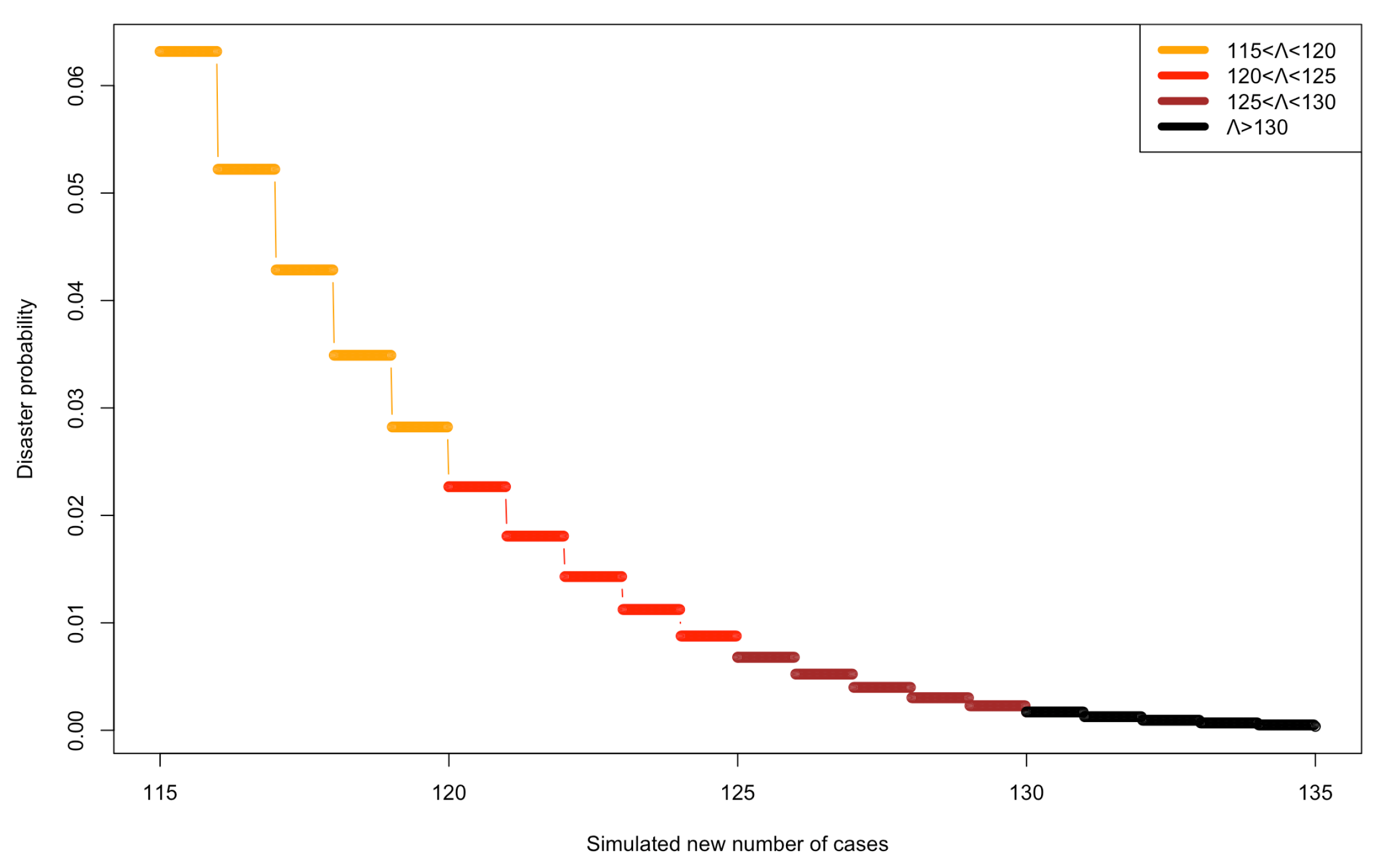
Figure 6 suggests that $p_t^{*}=P({\Lambda }_t>n^c)$9 decreases as investors realize higher ${\Lambda }_t$, in line with the fact that tail events are rare events with a lower probability of occurrence. Figure 7 shows that any increase in ${\Lambda }_t$ decreases $p_t^{*}$ and, as a result, implies a higher instantaneous investors’ updating probability ($p_t$) since ${\displaystyle \frac{\partial p_t}{\partial p_t^{*}}}<0$ (Section 3.1). By rewriting the condition as

$$Upper.Bound={\displaystyle \frac{1}{1-\frac{p_{t-2}}{p_{t-1}}}}.{\displaystyle \frac{1}{{\Lambda }_t}}.{\displaystyle \frac{B^{-\gamma }}{1-B^{-\gamma }}}.D_t({\varphi }^H-{\varphi }^L),$$

it can be easily proved that the upper bound is decreasing in terms of instantaneous COVID-19-intensity (${\Lambda }_t$), regardless of upward or downward IUP from $t-2$ to $t-1$. This means that the price differential increases under the tighter condition. In other words, an increase in COVID-19 intensity gives new information to investors, updates IUP upward, and tightens the price differential condition in a sense that the price differential increases if this differential was much smaller in the previous period.

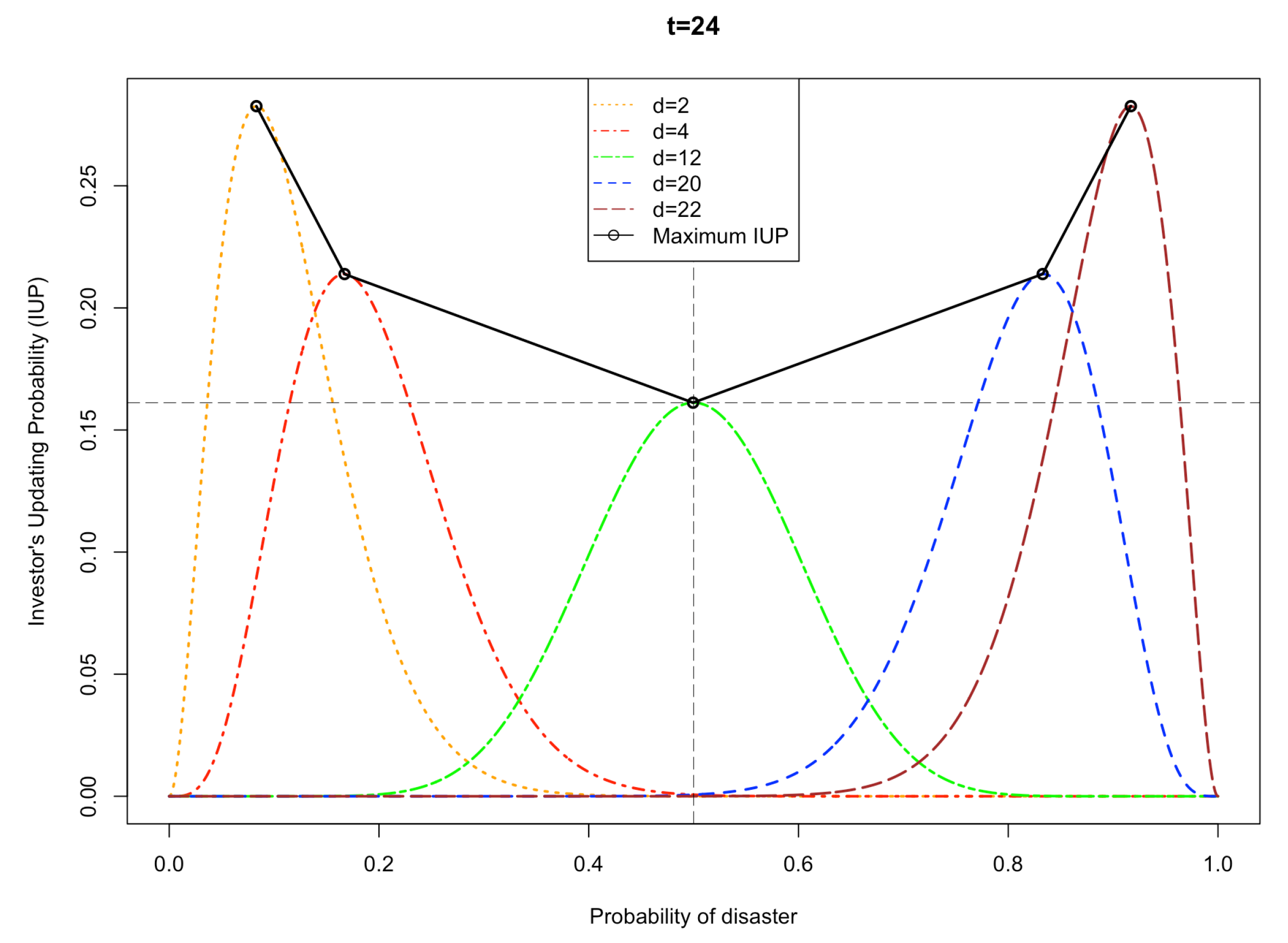
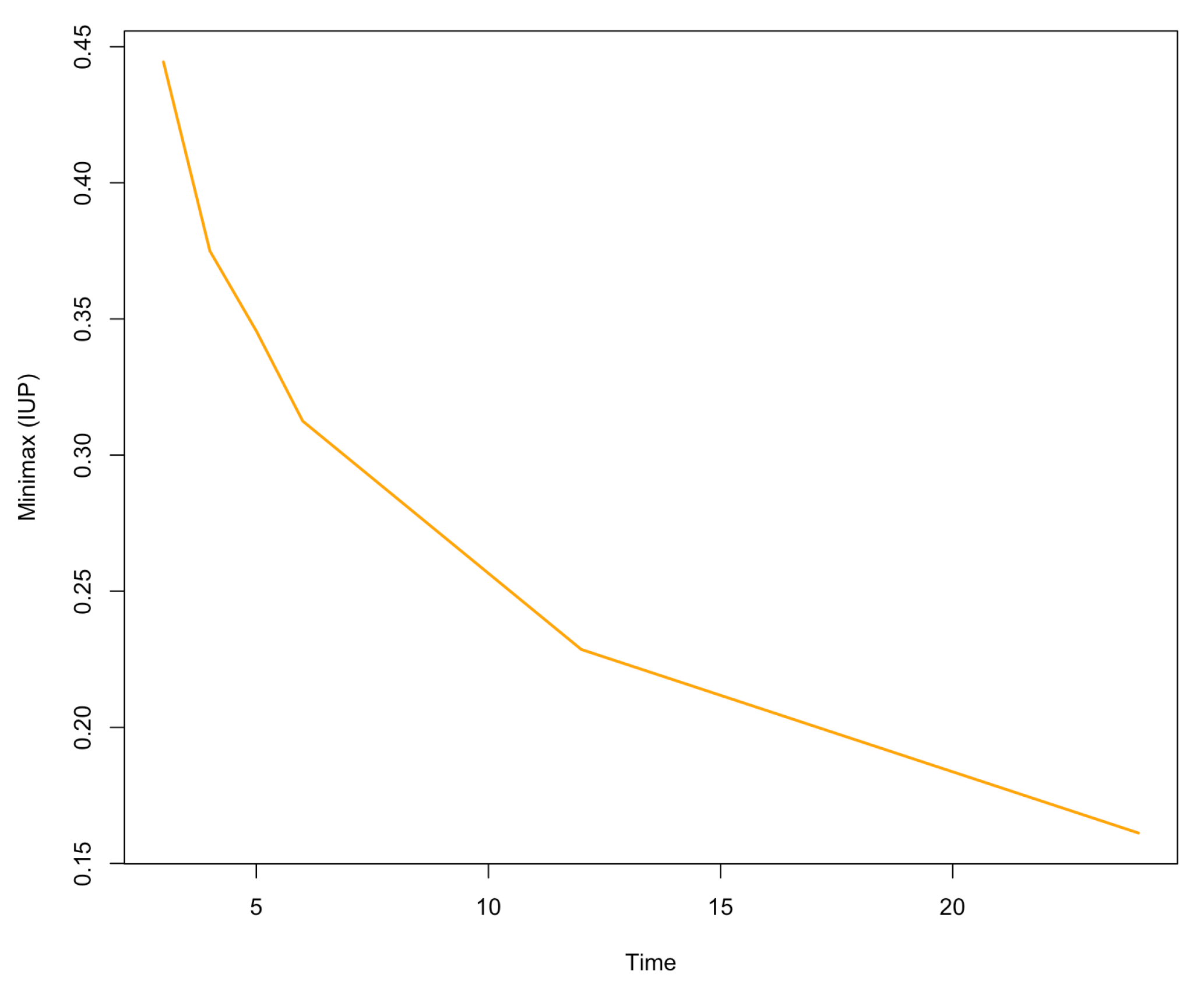
Furthermore, investors’ updating of disaster probability in two recent periods ($p_{t-1}$ and $p_{t-2}$) plays a key role in price differentials. One interesting feature is the implicit role of the number of disaster periods in the realized sequence in investors’ updating probability in these periods and the consequent upper bound of price differentials above. Consistently, as the number of disaster states increases in the pandemic era10, the maximum investors’ updating probability surges to one (Figure 2 and Figure 3). The key point here is that under the proposed conditions in Section 3.1 and in the disaster situation $(p_t^{*}>0.5)$, investors may update their beliefs upward, $(p_{t-2}<p_{t-1})$, or downward, $(p_{t-2}>p_{t-1})$, depending on resilience of the asset. This affects price movements in the current period and the corresponding upper bound and, as a result, the price differential trend in the following period. This evidence establishes the importance of disentangling investors’ updating probability and disaster probability.

This proposition shows how long-memory investors play a role in future price fluctuations and implies that even in the case of a no-disaster period, there is a process of learning in investors’ behavior, emphasizing the novelty and necessity of the proposed setup.

Proposition 2. 

High-resilience assets see fewer expected returns, as opposed to low-resilience ones, if

$${\displaystyle \frac{p_t}{1-p_t}}>\left({\displaystyle \frac{p_t^{*}}{1-p_t^{*}}}\right)B^{\gamma }.$$

This condition proposes a lower bound for investors’ updating probability (IUP) that is defined in a different way from disaster probabilities and remarks how this lower bound is related indirectly to COVID-19-intensity through disaster probability ($p_t^{*}$) and directly to risk aversion, $\gamma$. This lower bound can potentially be an answer to the flip points in the evolution of the expected returns of high- and low-resilience assets (Pagano et al. 2023).

Solving the maximization problem and first-order conditions with respect to $n_t^H$ and $n_t^L$ and replacing the equilibrium values of consumption in the marginal utility function yield the following expression for high- and low-resilience asset prices:

$$P_t^i=\left({\displaystyle \frac{D_{t+1}}{1+\delta }}\right){\displaystyle \frac{p_t[\frac{{\varphi }^H}{{\Lambda }_{t+1}}\left(\frac{1}{x}\right)-1]+1}{p_{t-1}[\frac{1}{x}-1]+1}},\phantom{hhhh}for\phantom{h}i=H,L.$$

Then, using the short-hand $x\equiv B^{\gamma }<1$, the expected return for high- and low-resilience assets in any period of t is

$$1+E\left(r_{t+1}^i\right)={\displaystyle \frac{E\left(D_{i,t+1}\right)}{P_t^i}}={\displaystyle \frac{p_t^{*}\frac{D_{t+1}}{{\Lambda }_{t+1}}{\varphi }^i+(1-p_t^{*})D_{t+1}}{\left(\frac{D_{t+1}}{1+\delta }\right)\frac{p_t[\frac{{\varphi }^H}{{\Lambda }_{t+1}}\left(\frac{1}{x}\right)-1]+1}{p_{t-1}[\frac{1}{x}-1]+1}}},\phantom{hhhh}for\phantom{h}i=H,L.$$

(2)

In any period t, it can clearly be seen that by differentiating the expected returns with respect to asset resilience, ${\varphi }^i$,

$$\begin{array}{cc}\hfill {\displaystyle \frac{\partial (1+E\left(r_{t+1}^i\right))}{\partial {\varphi }^i}}& =(1+\delta )[p_{t-1}({\displaystyle \frac{1}{x}}-1)+1]{\displaystyle \frac{1}{{[p_t(\frac{{\varphi }^i}{x{\Lambda }_{t+1}}-1)+1]}^2}}[{\displaystyle \frac{p_t^{*}}{{\Lambda }_{t+1}}}[p_t({\displaystyle \frac{{\varphi }^i}{x{\Lambda }_{t+1}}}-1)+1]\hfill \\ & -{\displaystyle \frac{p_t}{x{\Lambda }_{t+1}}}[1+({\displaystyle \frac{{\varphi }^i}{{\Lambda }_{t+1}}}-1)p_t^{*}]],\phantom{hhhh}for\phantom{h}i=H,L.\hfill \end{array}$$

This statement is negative if

$${\displaystyle \frac{p_t^{*}}{{\Lambda }_{t+1}}}(1-p_t)<{\displaystyle \frac{p_t}{x{\Lambda }_{t+1}}}(1-p_t^{*}),$$

Equivalently,

$${\displaystyle \frac{p_t}{1-p_t}}>\left({\displaystyle \frac{p_t^{*}}{1-p_t^{*}}}\right)x.$$

This inequality implies a lower bound for the odds ratio of investors’ updating probability, ${\displaystyle \frac{p_t}{1-p_t}}$. Specifically, it shows that more risk-averse investors, who change their perception about disaster probability more often than others, impose fewer expected returns for high-resilience assets. It is straightforward to show that in the case of any increase in risk aversion in $B^{\gamma }$ ($B>1$), the lower bound increases and suggests tighter conditions in a sense that the relative investors’ updating probability (${\displaystyle \frac{p_t}{1-p_t}}$) can potentially become much greater than the relative disaster probability (${\displaystyle \frac{p_t^{*}}{1-p_t^{*}}}$).

Moreover, the lower bound is positive in disaster periods when the relative resilience to the intensity of shock is at a very low level ($0<B<1$). This implies a wider condition for the perceived odds ratio of disaster by investors (${\displaystyle \frac{p_t}{1-p_t}}$), meaning that it is more possible to see that investors impose a higher probability for a disaster event than disaster probability itself. Obviously, this condition proves that in any case of B, there are fewer expected returns for high-resilience assets in a sense that these assets are less risky, in line with Daadmehr (2024).

Proposition 3. 

Regardless of having a disaster or no-disaster event in the period t, any increase in disaster intensity in the following period implies greater expected returns.

Using Equation (2), the expected returns of either high-resilience or low-resilience assets, $i=H,L$, is an increasing function of intensity: ${\Lambda }_{t+1}$:

$${\displaystyle \frac{\partial (1+E\left(r_{t+1}^i\right))}{\partial {\Lambda }_{t+1}}}=(1+\delta ){\displaystyle \frac{[p_{t-1}(\frac{1}{x}-1)+1]}{{(p_t(\frac{{\varphi }^i}{x{\Lambda }_{t+1}}-1)+1)}^2}}\left({\displaystyle \frac{{\varphi }^i}{{\Lambda }_{t+1}^2}}\right)[p_t^{*}(1-p_t)+p_t\left({\displaystyle \frac{1}{x}}\right)(1-p_t^{*})]>0.$$

This proposition reveals the instantaneous effect of COVID-19 intensity on expected returns. Investors expect more returns as soon as they observe a higher number of new deaths or new cases. The next proposition proves that such expectations increase severely for low-resilience assets.

Proposition 4. 

An increase in COVID-19 intensity increases the expected returns of low-resilience assets more than those of high-resilience ones.

According to Proposition 2, the following is the corresponding derivative of expected returns with respect to ${\Lambda }_{t+1}$ and ${\varphi }^i$:

$$\begin{array}{cc}\hfill {\displaystyle \frac{{\partial }^2(1+E\left(r_{t+1}^i\right))}{\partial {\varphi }^i\partial {\Lambda }_{t+1}}}& ={\displaystyle \frac{\partial }{\partial {\Lambda }_{t+1}}}[(1+\delta )[p_{t-1}({\displaystyle \frac{1}{x}}-1)+1]{\displaystyle \frac{1}{{[p_t(\frac{{\varphi }^i}{x{\Lambda }_{t+1}}-1)+1]}^2}}\left({\displaystyle \frac{1}{{\Lambda }_{t+1}}}\right)[p_t^{*}(1-p_t)\hfill \\ & +p_t\left({\displaystyle \frac{1}{x}}\right)(1-p_t^{*})]=(1+\delta )[p_{t-1}({\displaystyle \frac{1}{x}}-1)+1][p_t^{*}(1-p_t)+p_t\left({\displaystyle \frac{1}{x}}\right)(1\hfill \\ & -p_t^{*})]{\displaystyle \frac{1}{{[p_t(\frac{{\varphi }^i}{x{\Lambda }_{t+1}}-1)+1]}^3}}[3{\displaystyle \frac{p_{t}x{\varphi }^i}{{\Lambda }_{t+1}}}+(1-p_t)]\hfill \end{array}$$

The proposition is satisfied if $p_t^{*}(1-p_t)-p_t\left({\displaystyle \frac{1}{x}}\right)(1-p_t^{*})$ is less than zero (Proposition 2). Consequently, ${\displaystyle \frac{{\partial }^2(1+E\left(r_{t+1}^i\right))}{\partial {\varphi }^i\partial {\Lambda }_{t+1}}}$ is negative. This proposition provides a theoretical proof to show that the expected returns of low-resilience assets are instantaneously more sensitive to COVID-19 intensity, meaning that investors are more elastic to the return expectations in response to COVID-19 intensity for low-resilience assets. Investors asymmetrically expect many more returns for low-resilience assets when the economy is at risk of a higher number of new deaths or new number of cases.

It is noteworthy to mention that a similar statement is investigated for expected cash flows in a “different framework” by Daadmehr (2022).

Proposition 5. 

In any period t, as investors’ updating probability regarding disaster increases, the expected return increases.

Using Equation (2), the expected return with respect to $p_t$ is the following:

$$\begin{array}{cc}\hfill {\displaystyle \frac{\partial (1+E\left(r_{t+1}^i\right))}{\partial p_t}}& =(1+\delta )[p_{t-1}({\displaystyle \frac{1}{x}}-1)+1][1+({\displaystyle \frac{{\varphi }^i}{{\Lambda }_{t+1}}}-1)p_t^{*}]({\displaystyle \frac{1}{{(p_t(\frac{{\varphi }^i}{x{\Lambda }_{t+1}}-1)+1)}^2}})[p_t{\varphi }^i{\displaystyle \frac{1}{x{\Lambda }_{t+1}^2}}]\hfill \end{array}$$

which is always positive.

Proposition 6. 

Regardless of being in a disaster or no disaster in the period t, any increase in disaster intensity, ${\Lambda }_{t+1}$, leads to a greater expected return differential.

Using Equation (2), the expected return differential is the following:

$${\Delta }_{LH}\equiv {\displaystyle \frac{1+E\left(r_{t+1}^L\right)}{1+E\left(r_{t+1}^H\right)}}={\displaystyle \frac{1+(\frac{{\varphi }^L}{{\Lambda }_{t+1}}-1)p_t^{*}}{1+(\frac{{\varphi }^H}{{\Lambda }_{t+1}}-1)p_t^{*}}}\times {\displaystyle \frac{p_t(\frac{{\varphi }^H}{x{\Lambda }_{t+1}}-1)+1}{p_t(\frac{{\varphi }^L}{x{\Lambda }_{t+1}}-1)+1}}$$

(3)

Using Equation (3), the variation in the expected return differential with respect to ${\Lambda }_{t+1}$ is obtained as the following:

$$\begin{array}{cc}\hfill {\displaystyle \frac{\partial {\Delta }_{LH}}{\partial {\Lambda }_{t+1}}}& =({\displaystyle \frac{p_t(\frac{{\varphi }^H}{x{\Lambda }_{t+1}}-1)+1}{p_t(\frac{{\varphi }^L}{x{\Lambda }_{t+1}}-1)+1}}){\displaystyle \frac{1}{{(1+(\frac{{\varphi }^H}{{\Lambda }_{t+1}}-1)p_t^{*})}^2}}{p}_t^{*}({\displaystyle \frac{1}{{\Lambda }_{t+1}^2}})(1-p_t^{*})({\varphi }^H-{\varphi }^L)\hfill \\ & +({\displaystyle \frac{1+(\frac{{\varphi }^L}{{\Lambda }_{t+1}}-1)p_t^{*}}{1+(\frac{{\varphi }^H}{{\Lambda }_{t+1}}-1)p_t^{*}}}){\displaystyle \frac{1}{{(p_t(\frac{{\varphi }^L}{x{\Lambda }_{t+1}}-1)+1)}^2}}{p}_t({\displaystyle \frac{1}{x{\Lambda }_{t+1}^2}})(1-p_t)({\varphi }^L-{\varphi }^H).\hfill \end{array}$$

which is positive for

$$p_t(1-p_t)<x{\displaystyle \frac{{\Delta }_2}{{\Delta }_1}}{p}_t^{*}(1-p_t^{*})$$

where

$${\Delta }_1={\displaystyle \frac{1+(\frac{{\varphi }^L}{{\Lambda }_{t+1}}-1)p_t^{*}}{1+(\frac{{\varphi }^H}{{\Lambda }_{t+1}}-1)p_t^{*}}},$$

and

$${\Delta }_2={\displaystyle \frac{p_t(\frac{{\varphi }^H}{x{\Lambda }_{t+1}}-1)+1}{p_t(\frac{{\varphi }^L}{x{\Lambda }_{t+1}}-1)+1}}.$$

This proposition explains that depending on disaster probability and under some conditions for investors’ updating probability, a higher number of new cases or new deaths as an indicator of COVID-19 intensity implies an increase in the expected return differential between high- and low-resilience assets.

Proposition 7. 

An increase in investors’ updating probability regarding disaster results in greater revisions in the expected return differential.

According to Equation (3), the variation in the expected return differential with respect to $p_t$ is

$${\displaystyle \frac{\partial {\Delta }_{LH}}{\partial p_t}}=({\displaystyle \frac{1+(\frac{{\varphi }^L}{{\Lambda }_{t+1}}-1)p_t^{*}}{1+(\frac{{\varphi }^H}{{\Lambda }_{t+1}}-1)p_t^{*}}}){({\displaystyle \frac{1}{p_t(\frac{{\varphi }^L}{x{\Lambda }_{t+1}}-1)+1}})}^2{\displaystyle \frac{1}{x{\Lambda }_{t+1}}}({\varphi }^H-{\varphi }^L)>0,$$

which is positive since ${\varphi }^L<{\varphi }^H$. This proposition theoretically explains how the expected return differential is responsive to investors’ updating probability that itself depends not only on disaster probability by definition but also on COVID-19 intensity as a possible realization of the number of new cases or number of new deaths through the Poisson distribution (previous propositions).

Proposition 8. 

In any period t, the expected return increases as COVID-19 intensity increases.

Based on Equation (2), Proposition 5, and the condition of ${\displaystyle \frac{\partial p_t}{\partial p_t^{*}}}$ implying $p_t^{*}>{\displaystyle \frac{d_{t-1}}{t}}$ in no-disaster periods and $p_t^{*}>{\displaystyle \frac{d_{t-1}+1}{t}}$ in disaster periods (Section 3.1), the variation in the expected return with respect to COVID-19 intensity, ${\Lambda }_t$, is the following:

$${\displaystyle \frac{\partial (1+E\left(r_{t+1}^i\right))}{\partial {\Lambda }_t}}={\displaystyle \frac{\partial (1+E\left(r_{t+1}^i\right))}{\partial p_t}}\left({\displaystyle \frac{\partial p_t}{\partial p_t^{*}}}\right){\displaystyle \frac{\partial p_t^{*}}{\partial {\Lambda }_t}}={\displaystyle \frac{\partial (1+E\left(r_{t+1}^i\right))}{\partial p_t}}\left({\displaystyle \frac{\partial p_t}{\partial p_t^{*}}}\right)[{\displaystyle \frac{-{\left(\Lambda h\right)}^{n^c}{e}^{-\Lambda h}}{n^c!}}]>0.$$

and it is always positive.

Proposition 9. 

The expected return sensitivity to COVID-19 intensity in the period t increases as the average intensity rate of COVID-19 sees greater values.

Following Proposition 8,

$$\begin{array}{cc}\hfill {\displaystyle \frac{{\partial }^2(1+E\left(r_{t+1}^i\right))}{\partial \Lambda \partial {\Lambda }_t}}={\displaystyle \frac{\partial }{\partial \Lambda }}\left({\displaystyle \frac{\partial (1+E\left(r_{t+1}^i\right))}{\partial {\Lambda }_t}}\right)& ={\displaystyle \frac{\partial (1+E\left(r_{t+1}^i\right))}{\partial p_t}}\left({\displaystyle \frac{\partial p_t}{\partial p_t^{*}}}\right)\left({\displaystyle \frac{1}{n^c!}}\right)\hfill \\ & [-h{n}^c{\left(\Lambda h\right)}^{n^c-1}{e}^{-\Lambda h}-h{e}^{-\Lambda h}{\left(\Lambda h\right)}^{n^c}]>0.\hfill \end{array}$$

This proposition emphasizes the implicit role of the perceived average rate of COVID-19 pathological disease (average intensity of exogenous shock) on expected return revisions. It proves that when the overall rate of COVID-19 cases (or deaths) increases, the expected return is realistically more responsive to variation in the intensity of disaster.

Proposition 10. 

Higher COVID-19 intensity implies an increase in the expected return differential.

The variation in the expected return differential with respect to COVID-19 intensity, ${\Lambda }_t$, is the following:

$${\displaystyle \frac{\partial {\Delta }_{LH}}{\partial {\Lambda }_t}}={\displaystyle \frac{\partial {\Delta }_{LH}}{\partial p_t}}\times {\displaystyle \frac{\partial p_t}{\partial p_t^{*}}}\times {\displaystyle \frac{\partial p_t^{*}}{\partial {\Lambda }_t}}={\displaystyle \frac{\partial {\Delta }_{LH}}{\partial p_t}}[{\displaystyle \frac{{\left(\Lambda h\right)}^{n^c}{e}^{-\Lambda h}}{n^c!}}]>0.$$

According to Proposition 7 and Section 3.1, it is always positive. The proposition provides an implicit link between the type of disaster (pathological COVID-19 disease) and the characteristics of assets (workplace resilience). This theoretically tracks how the differential of the expected returns of assets categorized based on workplace resilience can be affected by more cases or new deaths as a proxy for COVID-19 intensity.

Proposition 11. 

The expected return differential sensitivity to COVID-19 intensity in the period t increases as the average intensity rate of COVID-19 hits a higher value.

Following Proposition 10,

$${\displaystyle \frac{{\partial }^2{\Delta }_{LH}}{\partial \Lambda \partial {\Lambda }_t}}={\displaystyle \frac{\partial }{\partial \Lambda }}({\displaystyle \frac{\partial {\Delta }_{LH}}{\partial {\Lambda }_t}})={\displaystyle \frac{\partial {\Delta }_{LH}}{\partial p_t}}({\displaystyle \frac{1}{n^c!}})[h{n}^c{\left(\Lambda h\right)}^{n^c-1}{e}^{-\Lambda h}+h{e}^{-\Lambda h}{\left(\Lambda h\right)}^{n^c}]>0.$$

which is always positive if the average intensity of shock ($\Lambda$) is less than ${\displaystyle \frac{n_c}{h}}$. As is explained in Proposition 10, this proposition similarly reveals the implicit role of the rate of COVID-19 pathological disease on the expected return differential. It proves that when the overall intensity rate of COVID-19 ($\Lambda$) increases, the expected return differential between high- and low-resilience assets is realistically more responsive to the variation in the current intensity of disaster.

These theoretical results highlight how pandemic intensity creates information and plays a role in investors’ updating beliefs with different probabilities depending on the probability of disaster and its prolongation. These results specifically emphasize the necessity of disentangling investors’ updating probability and disaster probability and the impact on expected returns.

Although including data-driven evidence (e.g., historical stock returns during the pandemic) would strengthen the credibility of the results, empirical analysis without enough data is not reliable. This paper did not use historical stock returns to avoid the contamination of the impact of previous crises (2011 European crisis, 2008 financial crises, 2005 SARS-CoV, and others like WW1 and WW2) since different types of disasters have different consequences on the economy or affect the economy with different mechanisms (Jordà et al. 2022). This limits the period of time, which is a very short period for (calibrating) such a detailed asset pricing model.

On the other hand, there were nine years (2013–2022) unaffected by the impact of any other crises, and more importantly, neither investors nor managers had learned from the impact of the previous pandemics (a severe market crash as explicit evidence). This redirected this paper to rationalize the evidence in other empirical studies by proposing the theoretical framework. This paper decided to work on how the pandemic affects expectations (expected returns).

In the period of a pandemic, especially with different mitigation policies like social distancing and lockdowns, the exogenous impact of COVID-19 on human interaction and the consequent impact on the workforce place this model in a completely different category of asset pricing models. This paper emphasizes the importance of proposing a trackable analytical characterization for heterogeneous expected returns. These propositions provide a theoretical specification for resilient heterogeneous expected returns and enable theoretically tracking how workplace resilience affects these expectations, which are vital for firms to adopt appropriate corporate policies.

Firms can optimize their performance and expected returns as a proxy by controlling corporate financials. For instance, corporate policies on cash holdings can influence expected returns. Firms with higher cash holdings tend to have higher expected equity returns, particularly if they have riskier cash flows like low-workplace-resilience firms (as Daadmehr (2022) empirically proves). In other words, firms can manage to alleviate the impact of social distancing rules and lockdowns on human interaction by having a higher level of cash holdings.

5. Conclusions

This paper proposes an interpretation of the relative behavior of the expected returns of high- and low-resilience assets and corresponding differentials in a pandemic disaster. It deviates from previous studies by considering “COVID-19 as a disaster”. It defines disaster probability based on COVID-19 intensity and the Poisson distribution. In the proposed framework, investors have longer memory and learn about the prolongation of the pandemic. By Bernoulli outcomes, this paper clarifies how investors’ updating probability is different from disaster probability. The setup explains the importance of this novelty and its impact on expected returns and their differentials.

This paper makes a new contribution to the literature and explicitly shows the necessity of conditions for increasing expected returns in terms of the degree of resilience, in a sense that there is a lower bound on the odds ratio of investors’ updating regarding a disaster, possibly explaining the flip points in the expected returns of high- and low-resilience assets provided by the existing empirical literature. The theoretical results present some evidence of the important role of COVID-19 intensity in relative price fluctuations in high- and low-resilience assets. Specifically, it shows that an increase in COVID-19 intensity increases the expected returns of low-resilience assets more than those of high-resilience ones.