The Impact of Nature Restoration Law on Equity Behavior: How Biodiversity Risk Affects Market Risk

Abstract

This study examines the market reaction to the approval of the Nature Restoration Law, a key component of the EU Biodiversity Strategy, and its implications for biodiversity-related financial risks. Using an event study methodology, we analyze the equity price movements of companies listed in the MSCI Europe Index that are equally weighted in relation to the announcement. We select the RepRisk Due Diligence Score, focusing on incidents linked to landscapes, ecosystems, and biodiversity, as a measure of biodiversity risk. At first, it seems that companies with a high RepRisk Due Diligence Score show limited or positive abnormal returns, suggesting that biodiversity risks are already priced for companies that have experienced incidents linked to this issue. Conversely, firms with lower biodiversity risk exposure see null or negative impacts, reflecting heightened investor concerns about new environmental regulations or compliance costs. Although the event does not have a systemic impact on European companies in the index, it seems that some sectors are affected when analyzed using parametric and non-parametric distributions.

1. Introduction

On Monday 17 June 2024, the Council of the European Union definitively approved the Nature Restoration Law1, a regulation for environmental protection that is part of the Green Deal, the ambitious European climate plan. European institutions had worked on it for over two years, but the law had a very complicated path due to resistance from many parties and countries. The new rules include the obligation to restore natural conditions to at least 20% of the land and sea surface of the European Union’s territories by 2030 to prevent their commercial exploitation; they also provide for the gradual extension of protection to all selected ecosystems by 2050. They will directly apply to member countries after publication in the Official Journal of the European Union. The event arguably increased both investor awareness about the loss of biodiversity and the prospect of, and uncertainty about, future biodiversity regulation or litigation.

This study aims to examine the reaction of the European stock market to the approval of the Nature Restoration Law and to analyze if the level of biodiversity risk of specific companies/sectors can affect this reaction. To this end, we follow the lead of Hamilton (1995), Klassen and McLaughlin (1996), Ramiah et al. (2013), and Kalhoro and Kyaw (2024) by using the technique of an event study to explore the effect of the new law’s approval. We want to provide evidence of whether biodiversity risk affects equity prices and whether market participants perceive the current pricing of biodiversity risk in equity markets.

This study aims to answer the following research questions:

RQ1: 

Has the Nature Restoration Law impacted equity prices in Europe?

RQ2: 

What is the role of issuers’ biodiversity risk in determining the impact of the Nature Restoration Law on equity prices?

RQ3: 

What is the role of the economic sector’s biodiversity risk in determining the impact of the Nature Restoration Law on equity prices?

To the best of our knowledge, the literature has not investigated the impact of the Nature Restoration Law on market risk or whether exposure to biodiversity risk is correlated with market risk.

This paper is divided into six sections, including the Introduction and Conclusions. Section 2 presents the literature on biodiversity risk and prior studies on the impact of green news and policy announcements. Section 3 describes the data and methodology. Section 4 and Section 5 disclose the results and a robustness test, respectively. The last section discusses the main implications of our findings for biodiversity risk in finance.

2. Literature Review

Biodiversity is the variability among living organisms from all sources including, inter alia, terrestrial, marine and other aquatic ecosystems and the ecological complexes of which they are part; this includes diversity within species, between species, and in ecosystems (CBD 1992). Drivers and pressures of biodiversity loss are changes in land and sea use, the direct exploitation of organisms, climate change, pollution, and invasive alien species. The loss of biodiversity and ecosystem services poses significant macroeconomic and financial risks and could result in economic shocks (Bosch 2022).

Academics and regulators have started to analyze possible ways to assess nature-related risks and integrate them into traditional financial risks. The first issue is measuring a financial portfolio’s dependence on one or more ecosystems. In this regard, Hadji-Lazaro et al. (2024) propose quantitative estimates of the dependencies on ecosystem services and the impacts on biodiversity of the security portfolio held by French financial institutions in 2019. Using the ENCORE database and the Global Biodiversity Score tool, they find that French financial institutions’ portfolios highly depend on ecosystem services, such as surface and groundwater provision, flood and storm protection, and climate regulation. Giglio et al. (2023) explore how biodiversity risks (both physical risks due to biodiversity loss and regulatory risks due to laws protecting biodiversity) affect economic activity and asset values by using Natural Language Processing techniques. Ma et al. (2024) construct a biodiversity risk index to investigate the impact of biodiversity risk challenges on the Chinese financial market. Naffa and Czupy (2024) find evidence of a biodiversity risk premium ranging between 0.9 and 3.6% of the maximum attainable Sharpe ratios of the analyzed universe. Flammer et al. (2025) present a framework for financing biodiversity through private and blended capital, emphasizing the monetization of biodiversity to attract investors.From a methodological point of view, several studies have focused on the impact of environmental regulations or ecological news on firm performance, with varying results. Hamilton (1995) employs event study analysis to show that news of high levels of toxic emissions leads to significantly negative abnormal returns. Konar and Cohen (1997) examine firm behavior in response to disclosures of Toxic Release Inventory emissions and find that firms announcing compliance with stringent environmental regulations experience positive abnormal stock returns, suggesting that the market perceives compliance as reducing future regulatory risks. Conversely, firms that fail to meet environmental standards often see adverse stock reactions, reflecting the anticipated costs of non-compliance, including fines and damage to reputation. Ramiah et al. (2015) examine how these green policies impact capital markets, focusing specifically on the response of U.S. industrial portfolios to the announcements of such policies. Using the event study methodology and asset pricing models, the analysis reveals that major polluting industries experience negative abnormal returns and increased systematic risk, while environmentally friendly businesses are less affected. Kalhoro and Kyaw (2024) examine investors’ reactions to biodiversity-related policy events, such as the 2021 Kunming Declaration and the UN Biodiversity Conference. Garel et al. (2024) find that, from 2019 to 2022, there is no clear link between the Corporate Biodiversity Footprint and stock returns. Still, after October 2021 (post-Kunming Declaration), firms with higher biodiversity impacts face declining stock values initially, followed by higher returns. This reflects the investor pricing of biodiversity-related risks, such as future regulations and litigation.

Ramiah et al. (2013) show that abnormal returns are associated with environmental regulations but argue that environmental policies do not achieve their desirable effects because heavy polluters (unlike non-polluters) are not affected negatively by stringent environmental policies. Electricity providers (among the largest polluters in Australia) are insensitive to these announcements, whereas industries such as the beverage sector (not considered heavy polluters) record negative abnormal returns.

Corporate social responsibility initiatives focusing on environmental performance have been another area of interest for event study research. Becchetti et al. (2023) investigate how media coverage of environmental, social, and governance (ESG) misconduct impacts the cost of equity, using data from 731 companies listed in the MSCI USA Index from 2007 to 2017. Among the three ESG categories, shareholders are most sensitive to social misconduct, meaning that media coverage of social issues (like labor relations or community impacts) tends to raise the cost of equity more than environmental or governance issues. Furthermore, the study shows that the cost of equity is even higher for companies with high ESG scores. Investors expect these companies to perform better in ESG terms, and any misconduct leads to a stronger negative reaction in financial markets.

Based on the previous literature, this study aims to test the hypothesis that introducing new biodiversity protection legislation has impacted stock prices. However, we expect that firms and/or sectors already exposed to biodiversity risk, because they are directly and extensively involved in the issue, are less impacted, as the prices of securities issued already discount a premium associated with sustainability risks. On the other hand, we intend to test the hypothesis that introducing stricter biodiversity protection regulations may have negatively impacted firms and/or sectors that are less directly involved in ecological concerns.

3. Data and Methodology

As explained by Cenedese et al. (2023), there are two principal ways of measuring biodiversity risks in the case of climate risks: one based on the actual footprint and another based on textual analysis. We used data from companies included in one of the most relevant European stock indexes, the MSCI Europe Index. Starting with the 415 constituents of the index at the end of May 2024, we excluded the companies for which Datastream do not provide values for historical prices, return on equity, total assets, CAPEX, total asset growth in 2023, book value per share, market value, or PPE/TA (property, plant, and equipment over total assets). These firm characteristics were selected following Garel et al. (2024). In the end, we had a total of 405 companies.

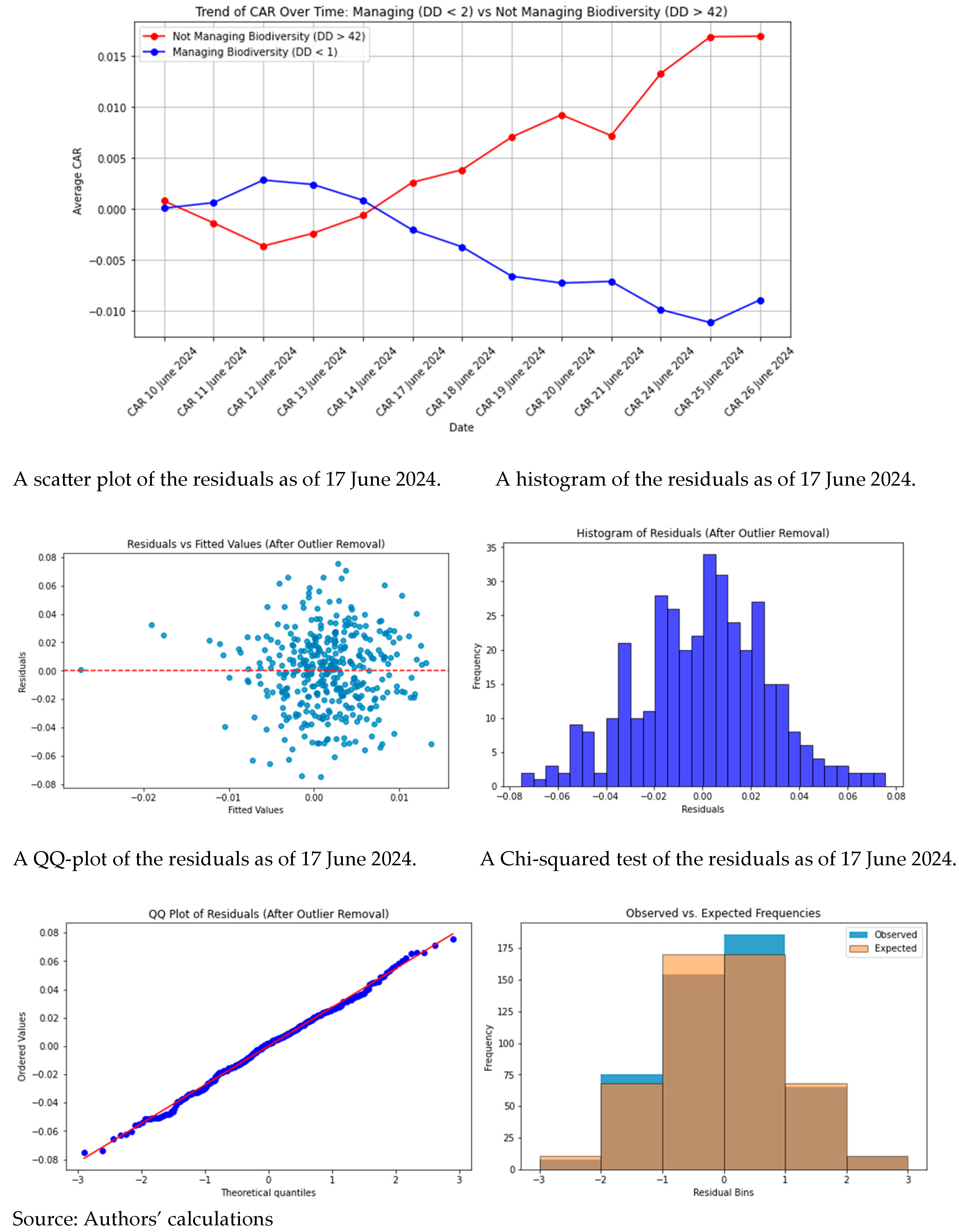
To assess the assumption of a normal distribution for daily returns, we produced a QQ-plot, a histogram, and a scatter plot of the residuals. Additionally, we performed a Chi-squared test to formally test normality.

However, on some dates, we observed high Jarque–Bera test values due to outliers. To address this, we applied winsorization and trimmed the residuals’ distribution’s top and bottom 20th percentiles.

We calculated daily returns using our sample companies’ first natural logarithmic difference in the underlying stock price. Following Benninga (2014), the expected returns were computed considering an estimation window of 252 trading days, from 23 June 2023 to 10 June 2024, with the Fama–French 3-factor model. The data relative to small-minus-big (SMB), high-minus-low (HML), and risk-free (RF) rate were taken from the Kenneth French data library.

To measure exposure to biodiversity risk, we used the daily RepRisk2 Due Diligence Score (DD Score) as of 17 June 2024, selecting only incidents linked to the ESG Issue Impacts on landscapes, ecosystems, and biodiversity from the RepRisk database with each identified ISIN code. RepRisk DD Scores measure a company’s compliance risk related to ESG issues. The score calculation is based on the RepRisk dataset, the world’s largest database of ESG risk incidents associated with companies and projects. The RepRisk dataset provides curated information on incidents reported by public sources and stakeholders and intentionally excludes company self-disclosures. DD Scores provide an outside–in assessment of ESG risks and serve as a reality check for how companies conduct their business. DD Scores range from zero (lowest) to 100 (highest), with higher values indicating higher risk exposure:

• 0–24: low risk.
• 25–49: medium risk.
• 50–59: high risk.
• 60–74: very high risk.
• 75–100: extreme risk.

The DD Score quantifies a company’s compliance risk regarding ESG issues. In our case, compliance risk concerns violating ESG norms or standards, particularly regarding landscapes, ecosystems, and biodiversity.

The formula for the score is as follows:

RepRisk Due Diligence Score = Average Incident Score × Normalized Incident Count

(1)

The Average Incident Score captures the average magnitude of non-compliance incidents, and the Normalized Incident Count measures the frequency/prevalence of the incidents. The magnitude of an incident is determined by considering its severity, reach, and recency (time of publication). A higher score is assigned to more recent incidents, incidents of greater severity, and those reported in sources with higher reach. The calculation involves the following weighted factors:

Incident Score = Severity weight × Reach weight × Time weight

(2)

where

(1)

Severity weights represent an incident’s environmental and societal impact. They grow exponentially with the assigned severity level. Less severe incidents are weighted as 1, severe incidents are weighted as 10, and very severe incidents are weighted as 100. Therefore, the severity weights increase exponentially with each severity level.

(2)

Reach weights help consider the credibility of the sources. The incidents reported in less credible sources are underweighted. Sources with medium and high reach (reach 2 and 3) have higher credibility than low-reach sources (reach 1). Thus, reach 1 sources are assigned a weight of 1, while reach 2 and 3 sources receive a weight of 2.

(3)

Time weights commonly take at least two years for a company to significantly reduce its ESG risk exposure, either through strategic, organizational, or managerial measures. Therefore, incidents are fully weighted in the first two years and then decay to a weight of 0 in years 2 to 4. Incidents older than four years receive a weight of 0, i.e., they do not contribute to the Incident Score.

Finally, the Average Incident Score is calculated as

$$\mathrm{A}\mathrm{v}\mathrm{e}\mathrm{r}\mathrm{a}\mathrm{g}\mathrm{e} \mathrm{I}\mathrm{n}\mathrm{c}\mathrm{i}\mathrm{d}\mathrm{e}\mathrm{n}\mathrm{t} \mathrm{S}\mathrm{c}\mathrm{o}\mathrm{r}\mathrm{e}={\displaystyle \frac{{\mathsf{\Sigma }}_i\mathrm{I}\mathrm{n}\mathrm{c}\mathrm{i}\mathrm{d}\mathrm{e}\mathrm{n}\mathrm{t} \mathrm{S}\mathrm{c}\mathrm{o}\mathrm{r}{\mathrm{e}}_i}{\mathrm{I}\mathrm{n}\mathrm{c}\mathrm{i}\mathrm{d}\mathrm{e}\mathrm{n}\mathrm{t} \mathrm{C}\mathrm{o}\mathrm{u}\mathrm{n}\mathrm{t}}}$$

(3)

The Normalized Incident Count quantifies the frequency of incidents associated with the company in the past four years. It aggregates the number of less severe (severity 1), severe (severity 2), and very severe (severity 3) incidents. The calculation applies a normalization factor to the count of less severe incidents. This corrects for potential selection bias (e.g., due to company size or location) and downscales the severity 1 Incident Count if it would overly inflate the score.

Normalized Incident Count = Normalization Factor × Severity 1 Incident Count + Severity 2 Incident Count + Severity 3 Incident Count

(4)

We use the RepRisk DD Score to proxy the exposure to biodiversity risk.

We next calculate the natural logarithm of returns as

$$D{R}_{i,t}=\mathrm{l}\mathrm{n}{\displaystyle \frac{P_{i,t}}{P_{1;t-1}}}$$

(5)

where DR_it is the daily return for the stock i at the time t, P_it is the price index for the stock i at the time t, and P_it−1 is the dividend-adjusted stock price index for the stock i at the time t − 1. Following Brown and Warner (1985), daily returns are adjusted by the Fama–French 3-factor model to obtain ex-post abnormal returns (AR_it) for each firm as follows:

AR_i,t = DR_i,t − E(R_i,t)

(6)

The daily expected return, E(R_it), is estimated by using an excess-return Fama–French 3-factor model over the past 252 observed daily returns:

E(R_it) = β₀ + β₁(r_mt − r_ft) + β₂SMB_t + β₃HML_t

(7)

The abnormal returns are then grouped into sectors to obtain the average sector (S) abnormal returns at the time t (ARS_t):

$$AR{S}_t={\displaystyle \frac{1}{N}}{\sum }_{1=1}^{N}A{R}_{it}$$

(8)

The cumulative abnormal return (CAR_it) measures the total abnormal returns during the event window. It is the sum of all the abnormal returns from the beginning of the event window until the end of the window.

$$CA{R}_{it} ={\sum }_{i=1}^{T}A{R}_{t_i}$$

(9)

According to the efficient market hypothesis (EMH), stock prices should immediately adjust to the latest information as soon as it becomes available, fully reflecting any relevant data. By examining abnormal returns, we can assess how the stock market responds on the first trading day after an announcement. However, critics of the EMH suggest that investors might not always respond rationally right away, and there could be lagged reactions (Chan 2003; Mcqueen et al. 1996). This can lead to instances where the market either overreacts or underreacts to new information, prompting corrections in the following days. To capture these potential adjustments, we define different event windows to also include any delayed reactions to the announcement: (0, +9); (−4, +2); (−5, +3); (−3, +9); and (−9, +9)3. These numbers refer to the days before and after the event date; they do not refer to trading days4. We choose these time windows since the Nature Restoration Law passed somewhat unexpectedly due to a last-minute change in voting decisions.

The standard t-statistic for evaluating an industry’s abnormal return helps determine if it significantly differs from zero. This leads to three possible scenarios:

(1)

The abnormal return (AR_it) equals zero.

(2)

The abnormal return (AR_it) is greater than zero.

(3)

The abnormal return (AR_it) is less than zero.

We interpret the AR during the event window as a measure of the event’s impact on the market value of security. We assume that the increase/decrease in biodiversity risk valuation drives a company’s abnormal returns. In scenario 1, the law’s approval does not cause any change in the price compared to the expected price. In scenario 2, the news of the approval leads to a price increase, likely due to reduced risk and the expectation of higher profits for the company. In scenario 3, the news causes a price drop, likely due to a perception of increased risk and higher future costs. We use the t-test to determine the statistical significance of absolute and cumulative returns. The standard t-statistic for a sector’s abnormal return is computed to determine whether it is statistically different from zero, giving rise to three outcomes: no abnormal return, a positive abnormal return, and a negative abnormal return. The efficient market hypothesis holds that stock prices reflect all available information and that information arrival through market surprises is incorporated in prices instantly. If the market is efficient, abnormal returns will only be observed on the first trading day. To cater for the potential delayed reaction, we estimate the cumulative abnormal return (CAR) over several trading days to find out whether the market reverts back to—or continues to deviate from—its expected value (Ramiah et al. 2013). Similarly to the abnormal return analysis, the t-test determines the statistical significance of cumulative returns.

Figure 1 demonstrates the progression of cumulative abnormal returns within the event window (−9, +9). In the days surrounding the event date, the blue line, representing companies that manage their biodiversity risk exposure (with a RepRisk DD Score less than 1, corresponding to approximately the top 35% of the distribution), consistently stays above the red line, which represents companies that do not manage their biodiversity risk exposure (with a RepRisk DD Score higher than 32 corresponding to approximately the 75th percentile). The graph indicates that companies that do not manage biodiversity (red line) experience a steady increase in the CAR, while those managing biodiversity (blue line) show a declining trend. This suggests that investors may perceive biodiversity management as a short-term cost, potentially penalizing these firms in the stock market.

We performed OLS regression for the different event windows, with the sector-level CARs as the dependent variable and the RepRisk DD Score (“DD”) as an independent variable. We also used the natural logarithm of total assets (TA), the return on equity (ROE), CAPEX, total asset growth in 2023, book value per share, market value, and PPE/TA as control variables.

4. Main Results

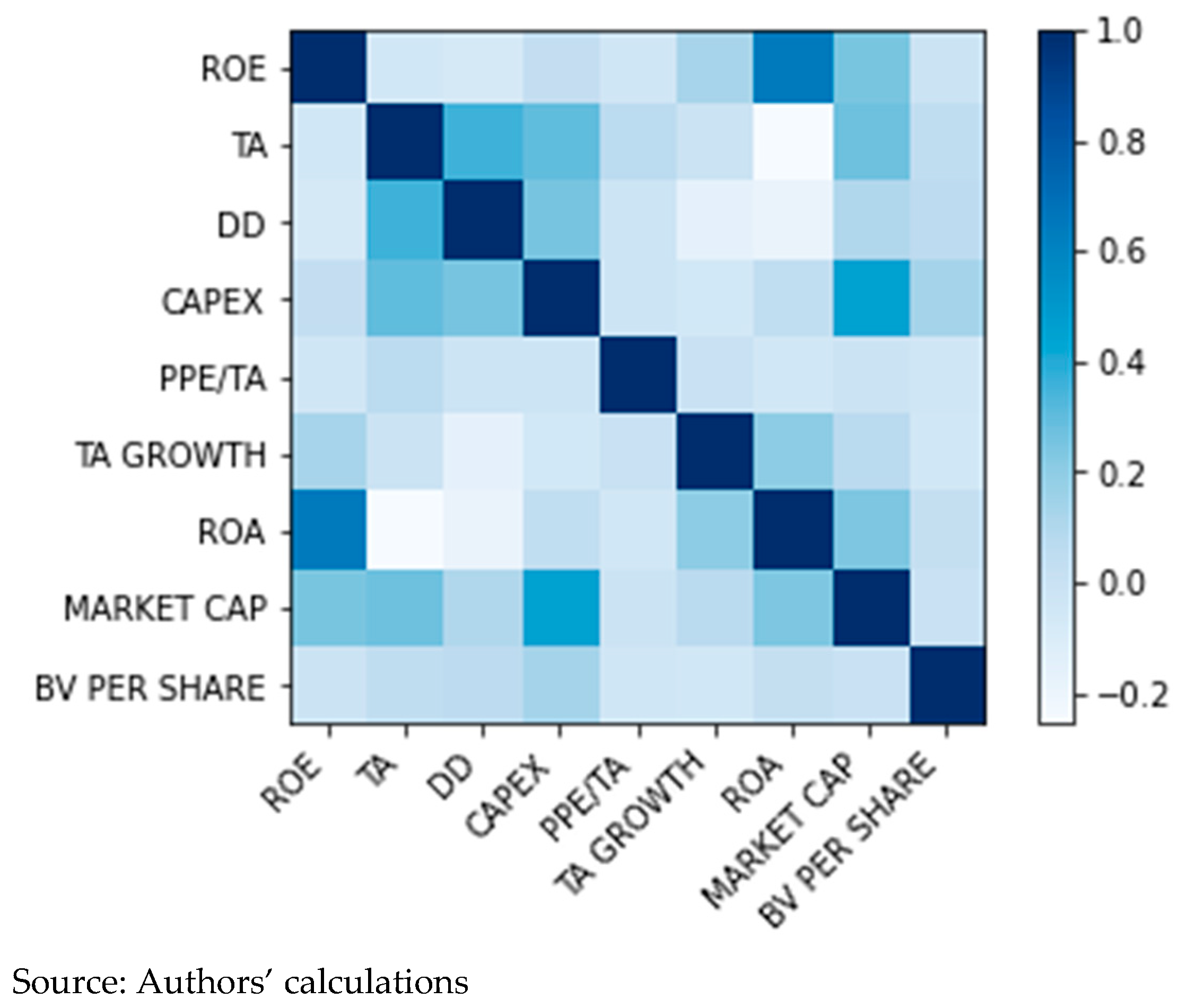
Firstly, to investigate the presence of potential multicollinearity issues, we constructed a correlation matrix for the aforementioned variables, shown in Figure 2. We can reasonably conclude that multicollinearity is not present.

When we ran a regression for all the companies in our sample, we obtained the results summarized in

Table 1. OLS regression for all companies.

ev Wind (0,+9)	18 June 2024	19 June 2024	20 June 2024	21 June 2024	24 June 2024	25 June 2024	26 June 2024
	0.0001 *	0.0002 **	0.0002 **	0.0001 *	0.0002 **	0.0004 ***	0.0004 ***
obs	392	388	388	386	386	387	387
R2	0.072	0.097	0.082	0.105	0.128	0.142	0.125
ev Wind (−3,+9)	19 June 2024	20 June 2024	21 June 2024	24 June 2024	25 June 2024	26 June 2024
	0.0002 **	0.0002 **	0.0002 **	0.0003 ***	0.0004 ***	0.0003 ***
obs	390	389	388	386	388	389
R2	0.102	0.106	0.112	0.146	0.156	0.160
ev Wind (−9,+9)	10 June 2024	11 June 2024	20 June 2024	24 June 2024	25 June 2024	26 June 2024
	0.06407 **	0.07569 **	0.0002 *	0.0003 **	0.0004 **	0.0003 **
obs	381	384	387	387	388	386
R2	0.068	0.089	0.048	0.087	0.105	0.106

Robust standard errors in parentheses. *** p < 0.01; ** p < 0.05; * p < 0.1.

. From these, we can hypothesize a positive trend before the law’s approval, with a slight effect (in the case of 20 June 2024, an increase in the DD Score by 1 leads to a decrease in the CAR for each day by 0.0002, with a significance level of 5%). In

Table 2. OLS regression for all companies on 17 June 2024 for event window (−9, +9).

OLS Regression Results
Dep. Variable:	CAR 18 June 2024	R-squared:	0.072
Model:	OLS	Adj. R-squared	0.050
Method:	Least Squares	F-statistic:	3.301
Prob (F-statistic):	0.000682
No. Observations:	392	AIC:	−1966
Df Residuals:	382	BIC:	−1926
	coef	std err	t	p > |t|	[0.025	0.975]
const	−0.0500	0.012	−4119	0.000	−0.074	−0.026
ROE	0.0001	0.000072	1506	0.133	−0.0000332	0.000
TA	0.0027	0.001	3855	0.000	0.001	0.004
DD	0.0001	0.0000578	1822	0.069	−0.00000834	0.000
CAPEX	0.0000	0.00000000016	−0.746	0.456	−0.000000000434	0.000000000195
PPE/TA	−0.0298	0.526	−0.057	0.955	−1063	1004
TA GROWTH	−0.000005	0.0000637	−0.077	0.938	−0.000	0.000
ROA	0.0002	0.000	0.931	0.353	−0.000	0.001
MARKET CAP	−0.0000000128	0.0000000017	−1874	0.062	−0.000000025	0.0000000006
BV PER SHARE	0.00	0.000000482	0.936	0.350	0.0000005	0.0000014
Omnibus:	2.661	Durbin-Watson:	1.913
Prob(Omnibus):	0.264	Jarque–Bera (JB):	2.679
Skew:	−0.199	Prob(JB):	0.262
Kurtosis:	2.930	Cond. No.	0.00000000404

, we can observe that not all the firms’ characteristics are significant variables. The level of significance changes from day to day, from sector to sector, and from subgroup to subgroup.

Considering the distribution of DD Scores within the sample, we classify companies into different groups based on very low or very high scores. Specifically, DD < 2 includes 151 observations, representing approximately the 35th percentile, while DD > 32 comprises 91 observations, corresponding to around 80% of the sample, and DD > 37 accounts for about 85%, with 61 observations. Given the asymmetric distribution, with a high concentration of DD Scores equal to zero, excluding these cases results in DD < 12 representing approximately the 15th percentile, DD < 17 covering around 20%, and DD > 42 making up roughly 80% of the sample. As outlined in

Table 3. OLS regression for companies grouped based on DD Score for each event window.

PLOT A
ev Wind (0,+9)		19 June 2024			24 June 2024			obs
DD < 1		0.0000000004845 *						146
DD < 2					−0.0280 *			151
DD < 12		0.0016 *						169
PLOT B
ev Wind (−3,+9)	17 June 2024	18 June 2024	19 June 2024	20 June 2024	21 June 2024	24 June 2024	25 June 2024	26 June 2024	obs
DD > 37	0.0006 **	0.0006 **	0.0007 *	0.0007 *	0.0010 **		0.0008 *	0.0009 *	61
DD > 42		0.0007 *				0.0011 **			51
PLOT C
ev Wind (−4,+2)		17 June 2024			19 June 2024			obs
DD < 12					0.0022 *			169
DD > 32		0.0005 **						91

Robust standard errors in parentheses. ** p < 0.05; * p < 0.1.

, companies with low DD values (DD < 1, DD < 2) generally experienced negative CARs, particularly on 24 June 2024 (−0.0280, significant at p < 0.05), suggesting that investors penalize firms with high biodiversity engagement. In contrast, firms with higher DD values (DD > 32; DD > 37; DD > 42) consistently showed positive and significant CARs over multiple days, with returns increasing over time, reaching 0.0011 on 24 June 2024 (p < 0.01) for DD > 42. Across different event windows, the trend remains quite consistent. In the (0,+9) window, firms with very low DD values (<1, <2) showed negative CARs, while firms with DD < 12 experienced slightly positive returns. In the (−3, +9) window, firms with DD > 37 and DD > 42 demonstrated significant positive CARs, reflecting sustained investor confidence. The (−4, +2) windowfurther supports this trend, with both DD < 12 and DD > 32 showing positive CARs, though higher-DD firms (DD > 32: 0.0005; p < 0.01) outperformed those with lower DD values (DD < 12: 0.0022; p < 0.05).

According to our main results, the introduction of the Nature Restoration Law seemed to have a positive impact on companies already exposed to biodiversity risk (represented by a high RepRisk DD Score). On the other hand, the regulation negatively impacted less exposed companies, especially in the few days following the event. Therefore, in cases with a strong risk signal already recorded by the market (high RepRisk DD Score), the new regulation did not significantly impact investors’ risk perceptions. On the contrary, companies that had not yet registered environmental and biodiversity incidents were negatively impacted by more severe legislation in this area, as investors’ perception of biodiversity risk may have increased for companies that had so far been considered to be little affected by the issue.

We then grouped the companies in subsamples by sector and conducted OLS regression.

Table 4. OLS regression for each event windows.

PLOT A

ev Wind (0,+9)

17 June 2024

18 June 2024

19 June 2024

20 June 2024

21 June 2024

24 June 2024

25 June 2024

26 June 2024

DD Avg

Automobiles and Parts

0.0016 *

0.0021 **

0.0019 **

35.54

Alternative Energy

−0.0026 *

31.77

Banks

0.0005 **

0.0005 **

0.0005 **

31.24

Chemicals

0.0005 **

0.0007 *

0.0008 **

26

Financial Services

0.0003 ***

0.0005 ***

0.0006 ***

0.0008 ***

0.0009 ***

0.0010 ***

0.0009 ***

0.0009 ***

14.05

Industrial Engineering

0.0009 **

9.9

Insurance

0.0006 *

0.0008 **

19.32

Personal and Household Goods

−0.0008 **

−0.0009 **

−0.0008 **

−0.0006 *

21.1

Pharmaceuticals and Biotechnology

−0.0008 *

0.0026

0.0030 *

0.0032 *

9.55

Retail

−0.0017 **

12.52

Software and Computer Services

0.0016 **

0.0016 **

0.0044 **

0.0048 **

0.0048 **

0.0049 *

6.43

Technology Hardware and Equipment

0.0009 **

0.0012 *

9.16

PLOT B

ev Wind (−3,+9)

14 June 2024

17 June 2024

18 June 2024

19 June 2024

20 June 2024

21 June 2024

24 June 2024

25 June 2024

26 June 2024

DD Avg

Aerospace and Defense

0.0031 **

14.82

Alternative Energy

−0.0031 **

31.77

Banks

0.0004 *

0.0003 *

31.24

Chemicals

−0.0004 **

26

Financial Services

0.0004 ***

0.0005 ***

0.0006 ***

0.0008 ***

0.0007 ***

0.0010 ***

0.0009 ***

0.0010 ***

14.05

Industrial Transportation

0.0005 *

0.0006 *

0.0014 *

0.0008 **

0.0010 *

24.06

Industrial Engineering

−0.0004 *

9.9

Insurance

0.0007 *

19.32

Personal and Household Goods

0.0005 *

21.1

Pharmaceuticals and Biotechnology

0.0027 **

0.0031 **

0.0033 **

9.55

Retail

−0.0012 *

12.52

Software and Computer Services

0.0039 ***

0.0043 **

0.0043 **

0.0044 **

6.43

Technology Hardware and Equipment

0.0006 *

9.16

PLOT C

ev Wind (−4,+2)

13 June 2024

17 June 2024

18 June 2024

19 June 2024

DD Avg

Alternative Energy

−0.0026 *

−0.0034 **

31.77

Financial Services

−0.0002 **

0.0004 *

0.0005 **

14.05

Industrial Transportation

0.0009 *

0.0007 **

0.0008 **

24.06

Pharmaceuticals and Biotechnology

0.0004 *

9.55

Software and Computer Services

−0.0013 ***

6.43

Utilities

0.0005 *

31.45

PLOT D

ev Wind (−5,+3)

12 June 2024

13 June 2024

14 June 2024

17 June 2024

18 June 2024

19 June 2024

20 June 2024

DD Avg

Alternative Energy

−0.0050 **

−0.0048 ***

31.77

Banks

−0.0003 **

−0.0004 **

31.24

Financial Services

0.0005 **

0.0007 ***

0.0006 **

14.05

Industrial Transportation

−0.0006 ***

24.06

Industrial Engineering

0.0008 **

0.0011 **

9.9

Insurance

−0.0003 **

−0.0005 **

−0.0008 *

−0.0008 *

19.32

Software and Computer Services

0.0035 *

6.43

Support Services (Industrial Goods and Services)

0.0031 **

0.0033 **

0.0028 *

9

Telecommunications

−0.0016 *

10.07

PLOT E

ev Wind (−9,+9)

10 June 2024

12 June 2024

13 June 2024

17 June 2024

18 June 2024

19 June 2024

20 June 2024

21 June 2024

24 June 2024

25 June 2024

26 June 2024

DD Avg

Alternative Energy

−0.0078 *

−0.0076 ***

−0.0077 ***

−0.0086 ***

−0.0094 ***

−0.0092 ***

31.77

Banks

−0.0004 *

31.24

Financial Services

0.0007 *

0.0006 *

0.0007 *

14.05

Insurance

−0.0005 *

−0.0008 *

19.32

Pharmaceuticals and Biotechnology

−0.0012 *

−0.0018 **

9.55

Support Services (Industrial Goods and Services)

−0.0006 **

0.0033 **

0.0035 **

9

Robust standard errors in parentheses. *** p < 0.01; ** p < 0.05; * p < 0.1.

, PLOT A, B, C, D, and E, summarize the results for the event windows (0, +9), (−3, +9), (−4, +2), (−5, +3), and (−9, +9), respectively.

The event study results reveal heterogeneous market reactions to the Nature Restoration Law across different industries. Some sectors, such as Industrial Transportation and Automobiles and Parts, exhibited positive and statistically significant coefficients, suggesting that investors may have already priced in the higher costs for companies belonging to sectors with high average DD Scores. In contrast, Alternative Energy, Retail, and Personal Household and Goods showed negative market reactions, likely reflecting concerns over increased regulatory costs and operational constraints. Additionally, companies with higher DD Scores (indicating greater exposure to biodiversity-related risks) tended to experience more pronounced stock price movements. However, some economic sectors did not have significant values across all event windows. More importantly, some sectors include only a small number of companies, which may contribute to some distortions in the results. In addition, the sector analysis shows that the market reaction was not strictly related to the sector’s average DD Score. This can be due to different factors. First, companies can be characterized by different DD Scores within a sector. These scores are related to incidents in which a specific company is involved. The results then reflect the average DD Scores of companies within the same sector, which may mitigate certain effects. Unfortunately, some sectors lack a number of companies in the subsample to sufficient perform a valid OLS regression test. Therefore, the analysis is useful to highlight trends and significant effects on some sectors. 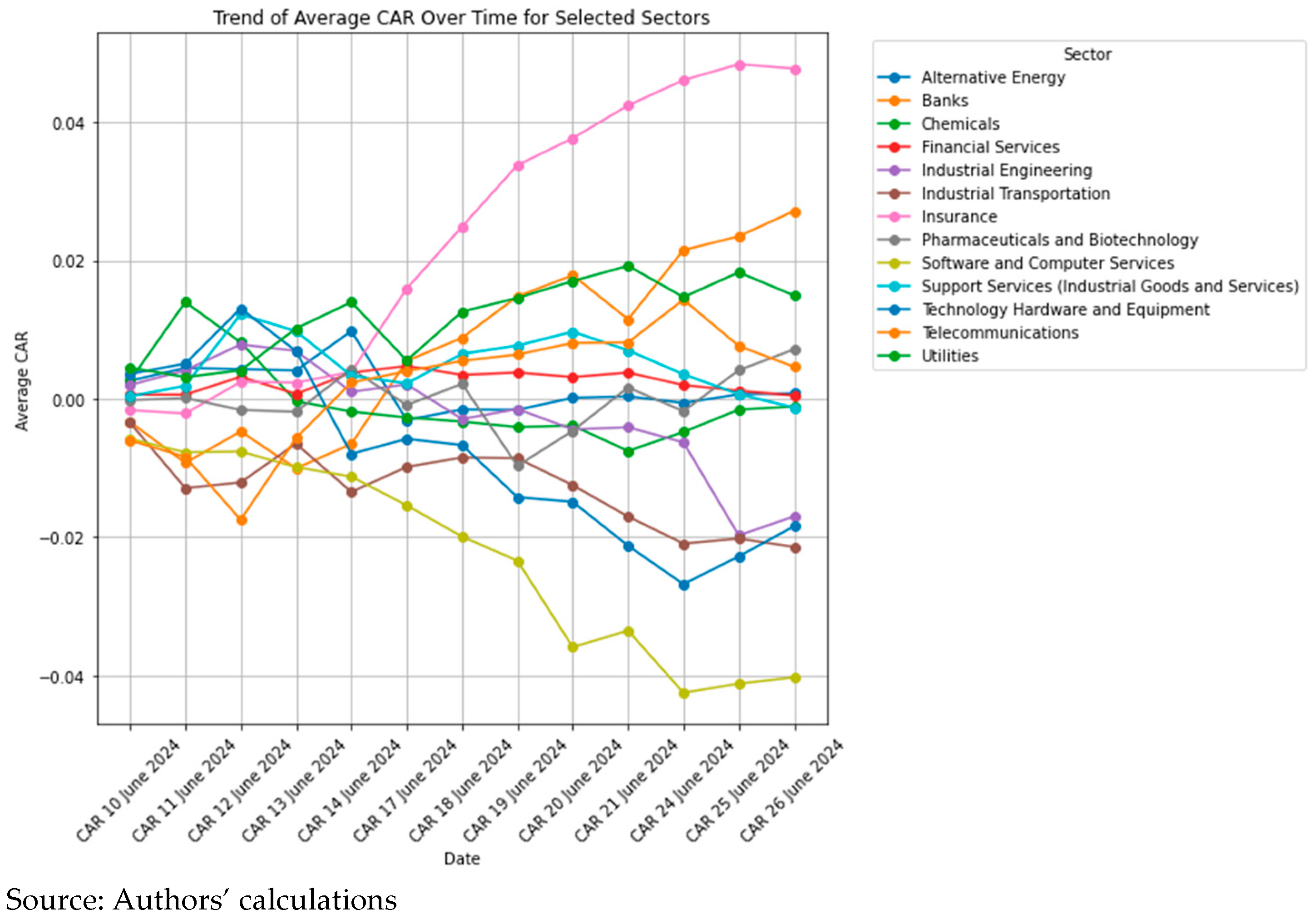To this end, Figure 3 shows the trend of the average CAR over time by selected sectors.

The graph illustrates different sectors’ varying market reactions to the Nature Restoration Law. Some industries, such as Insurance and Banks, exhibited a steady increase in cumulative abnormal returns (CARs) over time. In contrast, Software and Computer Services and Technology Hardware and Equipment experienced a sharp decline in the CAR, with a progressive drop over the event window. This seems to suggest that investors expected increased costs or regulatory burdens for companies belonging to this sector. Meanwhile, sectors such as Chemicals, Pharmaceuticals, and Biotechnology exhibited fluctuations around the zero-CAR level, indicating either limited market impact or uncertainty regarding the regulation’s effects. The graph further highlights that initial reactions were relatively small, with the divergence between positively and negatively impacted sectors becoming more pronounced over time.

5. Robustness Tests

We performed different robustness tests to validate the results just discussed. Assuming the hypothesis of a normal distribution of returns, we estimated the average returns and volatility during an estimation period of 252 days preceding the event date.

We considered two event windows: (0, +5) and (0, +9). Let “m” be the average returns in the estimation period and “D” be the standard deviation of these returns. We defined a range:

• lower_bound = (m − D)
• upper_bound = (m + D)

We then checked how many returns within the event window fell outside this range:

• outside_count = ((event_returns < lower_bound) | (event_returns > upper_bound))

For the (0, +5) window, we obtained 471 values out of 1620, representing 29%, where the companies’ returns fell outside the estimated historical range. The correlation between the number of cases outside the range and the DD Score was 0.019. For the (0,+9) event window, we had 742 values outside the range out of 3240 (22.9%). In this case, the correlation rose to 0.0236. This was particularly true for companies in Travel and Leisure, Banking, Insurance, Support Services, Health Care, Construction, and many other sectors.

Assuming normality, the entropy of the normal distribution of returns is given by

$$\mathrm{S}=\ln \left(\mathsf{\sigma }\sqrt{2\mathsf{\pi }\mathrm{e}}\right)\mathrm{or} \mathrm{S}={\displaystyle \frac{1}{2}}\ln \left(2\mathsf{\pi }\mathrm{e}\right)\mathrm{if} \mathsf{\sigma }$$

(10)

We conducted an analysis similar to the previous one, but now the range was given by the following:

• lower_bound = m − S
• upper_bound = m + S

In the case of the entropy of the normal distribution, in the (0,+5) event window, we found that the number of cases outside the range was 135 out of 1620 (8.33%), much lower than the previous one. The correlation in this case was negative, −0.10132. For the event window (0,+9), we had 216 cases out of 3240 (6.66%) and a correlation of −0.09184. In particular, we found results outside the range for companies in the following sectors: Software and Computer Services, Chemicals, Telecommunications, Pharmaceutical and Biotechnology, Industrial Transportation, Industrial Engineering, Retail, and Health Care Equipment and Services.

Following Ramiah et al. (2013), we employed two non-parametric tests as robustness tests to assess the effects of an event on the MSCI EU Index components: the Corrado non-parametric test (Corrado 1989) and the Kernel Density Estimation (KDE). These two non-parametric tests generally confirm results obtained with OLS regression. For further details, refer to Appendix A.

Finally, as a placebo test, we conducted a similar event study using a few test dates and applied it to the same overall sample. Considering the entire sample, no significant effects were found on any date.

Lastly, as in Garg et al. (2022), we employed a GARCH(1,1) model to analyze the volatility dynamics. We selected from 23 June 2023 to 9 June 2024 (Period 1) and from 10 June 2024 to 26 June 2024 (Period 2). The analysis used daily log returns, ensuring stationarity via the Augmented Dickey–Fuller (ADF) test before model estimation. The GARCH(1,1) model was fitted to each period, extracting key volatility parameters: omega (ω) represented baseline volatility, alpha (α₁) measured the impact of recent shocks, and beta (β₁) captured the persistence of volatility. Furthermore, the half-life of volatility decay was computed to assess market efficiency. As shown in

Table 5. GARCH(1,1) test.

Period	Omega	Omega p-Value	Alpha [1]	Alpha p-Value	Beta [1]	Beta p-Value	Half-Life
23 June 2023 to 9 June 2024	0.00000078	0	0.05	0.18915191	0.93	0	34.30937
10 June 2024 to 26 June 2024	0.0000064	0	0.01	0.963724835	0.889997	0.000183719	6.578575

, the results indicated an increase in the baseline volatility (ω) from 7.71 × ${10}^{-7}$(Period 1) to 6.37 × ${10}^{-6}$ (Period 2), suggesting heightened market uncertainty. However, the sensitivity to new shocks (α₁) declined from 0.05 to 0.01, and its statistical insignificance (p > 0.05) implies that daily market fluctuations had a diminished impact on overall volatility. Meanwhile, volatility persistence (β₁) remained high, though it slightly decreased from 0.93 to 0.89, indicating that while volatility remained persistent, it seemed to dissipate more quickly. This finding was reinforced by the half-life of volatility decay, which dropped significantly from 34.31 days to 6.58 days, suggesting that the market now absorbs information more efficiently and reverts to stability faster. These results suggest a trade-off between increased market volatility and improved efficiency. While the market has become more volatile, the faster dissipation of volatility shocks indicates a more adaptive and efficient market environment. This aligns with financial market theories suggesting that greater information flow and active trading can lead to higher volatility and faster stabilization. Future research could investigate the underlying macroeconomic or financial events contributing to these changes and explore potential sector-specific volatility trends.

6. Conclusions

This study investigates the impact of the Nature Restoration Law, a pivotal environmental regulation under the EU Biodiversity Strategy, on the equity prices of companies listed in the MSCI Europe Index. We use an event study methodology consistent with approaches documented in the existing literature. Evidence shows abnormal returns associated with different event windows. To measure the exposure to biodiversity risk, we use the daily RepRisk Due Diligence Score as of 17 June 2024, selecting only incidents linked to the ESG Issue Impacts on landscapes, ecosystems, and biodiversity from the RepRisk database.

For companies already exposed to significant biodiversity risk, as indicated by a high RepRisk Due Diligence Score, the introduction of the Nature Restoration Law either had a limited impact or resulted in positive market reactions.

In contrast, companies with lower biodiversity risk exposure experienced a null or, in some cases, a negative effect following the approval of the regulation.

This suggests that in cases where biodiversity risk was already recognized, the regulation did not substantially alter investor perceptions. However, for companies with previously lower perceived risk, the new law may have heightened concerns, leading to an increase in the perceived riskiness of the stocks.

While, on the one hand, the event did not have a systemic impact on European companies in the index, on the other hand, some sectors were found to be affected when analyzed using both parametric and non-parametric distributions. At the sector level, the results reveal divergent market reactions. Sectors such as Industrial Transportation and Automobiles and Parts showed positive and statistically significant coefficients, suggesting that investors may have already accounted for the regulatory impact on industries with high exposure to biodiversity risks. Conversely, sectors like Alternative Energy and Personal Household and Goods exhibited negative market reactions, likely reflecting concerns over higher regulatory costs and stricter compliance requirements.

Despite these findings, this study also highlights that market reactions were not strictly linked to the sector’s average DD Score and the impact observed was low. This could be attributed to the variability of DD Scores within each sector, where some companies may have faced higher biodiversity risks than others. Additionally, some sectors lacked enough companies in the sample, which may have influenced the overall results. This study highlights the growing importance of biodiversity risks in financial markets and underscores the significant role of regulatory changes in shaping investor sentiment. The results indicate that while markets may anticipate and price risks for high-exposure companies, unexpected regulatory shifts can still lead to substantial adjustments for less-exposed firms.

While this study provides valuable insights, especially about the set of companies analyzed (i.e., those included in the equally weighted MSCI Europe index), it also presents several limitations. One key limitation is the heterogeneity within industries, which makes it difficult to draw sector-wide conclusions, as individual firms may have different risk exposures despite belonging to the same industry. Additionally, some sectors contain only a small number of companies, which may limit the robustness of the OLS regression results and contribute to statistical distortions. Furthermore, the analysis primarily focuses on short-term market reactions, while the long-term implications of the Nature Restoration Law on stock performance remain uncertain and require further investigation. Finally, while the RepRisk DD Score captures past biodiversity incidents, it may not fully reflect investors’ expectations or perceptions regarding future regulatory risks. This could partially explain why companies with high DD Scores did not experience significant impacts.

To enhance the robustness of the findings and address these limitations, incorporating additional ESG risk indicators alongside the RepRisk Due Diligence Score could provide a more comprehensive assessment of biodiversity-related financial risks. Lastly, this study focused exclusively on the approval date of the Nature Restoration Law. However, future research could explore alternative key dates, such as its entry into force or its publication in the Official Journal, as these may also have significant financial implications.

These findings contribute to the growing literature on nature-related financial risks and highlight the need for the continued integration of biodiversity considerations into corporate and investment decision-making frameworks. To correctly price biodiversity risk, regulators should introduce incentives for biodiversity-compliant companies so that the implementation of new laws does not merely represent an additional cost. This would ensure that the regulatory burden is not only perceived as a financial penalty, which may already be priced in for non-biodiversity-compliant companies.