Forecasting Volatility of the Nordic Electricity Market an Application of the MSGARCH

Abstract

This paper studies the volatility of electricity spot prices in the Nordic market (Sweden, Finland, Denmark, and Norway) under regime switching. Utilizing Markov-switching GARCH (Generalized Autoregressive Conditional Heteroskedasticity) models, we provide strong evidence of nonlinear regime shifts in the volatility dynamics of these prices. Using in-sample criteria, we find that regime-switching models have lower AIC (Akaike information criterion) than single-regime GARCH models. In addition, out-of-sample forecasts indicate that regime-switching GARCH models have superior Value-at-Risk (VaR) prediction ability relative to single-regime models, which is directly pertinent to risk management. These findings highlight the importance of incorporating regime shifts into volatility models for accurately assessing and mitigating risks associated with electricity price fluctuations in deregulated markets.

1. Introduction

Electricity price forecasting has gotten much attention in the literature during the previous few decades. Since Nord Pool is one of the world’s most prosperous deregulated electricity markets, this market has attracted a lot of interest over the years. Additionally, it has a very active derivatives market.

The Nordic electricity market was rated as one of the world’s most effective regional electricity markets (Chen et al. 2021). Since the Nord Pool market was established in the early 1990s, supply security has been extremely high, and Nordic wholesale power costs have historically been among the lowest in Europe. There is adequate electricity supply in the Nordic market in terms of power generation capacity. As one of Europe’s top suppliers of electrical power, we therefore examine this market. Notably, several recent publications have clarified the significance of identifying jumps in the power market. For instance, (Ren et al. 2023) suggested that electricity prices exhibit extremely high volatility and that significant jumps are the primary characteristic of power markets. Such price increases and spikes occur in the spot market because of load variations, generating outages, or transmission breakdowns. Therefore, using a volatility model to capture jumps is crucial. Additionally, (Naeem et al. 2019) demonstrated that the Markov-switching GARCH model outperforms the conventional GARCH. A non-parametric model was recently used by (Dong et al. 2019) to investigate the volatility and jump dynamics of power prices in Denmark and Sweden. Their results show that because hydropower is a more reliable energy source, electricity costs are more constant in Swedish price regions. The fact that Nordic nations often have longer winters and slightly colder summers is also significant (Dong et al. 2019). This results in differing demand-side patterns. Additionally, the major usage of renewable energy in the process of producing electricity tends to have a significant influence on the variety in power prices. These price movement features have the potential to cause significant increases in Nordic power prices, which must be taken into account for more precise risk management and accurate forecasting of future electricity prices. To predict conditional volatility, the Generalized Autoregressive Conditional Heteroscedasticity (GARCH) model developed by (Bollerslev 1986) is frequently utilized (Hasanov et al. 2024; Queiroz and David 2023). For skewed data, the typical GARCH models may yield biased conclusions (Franses and Van Dijk 1996). The Glosten–Jagannathan–Runkle GARCH (GJR-GARCH) and Exponential Generalized Autoregressive Conditional Heteroskedastic (EGARCH) models are recommended for modeling volatility to solve this issue (Nelson 1991; Glosten et al. 1993; Szczygielski and Chipeta 2023). The conditional volatility of many financial time series has structural breaks, and disregarding this characteristic can significantly reduce the accuracy of volatility projections. As a result, considering structural changes could lead to better predicting performance (Hillebrand 2005; Teterin et al. 2016). Cai (1994) and Hamilton and Susmel (1994) added the regime-switching process to the GARCH model to account for potential structural changes. A discrete latent variable can cause Markov-switching GARCH models (MSGARCH) to change their return process over time. These models’ ability to quickly respond to changes in the level of unconditional volatility increases risk forecasting (Marcucci 2005; Ardia et al. 2018).

In this study, the MSGARCH package in R-4.4.1 software has been used which was developed by Ardia et al. (2019) and based on the research conducted by Haas et al. (2004a). To the best of our knowledge, the MSGARCH package has not been used for electricity spot prices of the Nord Pool region for risk management. Moreover, Amaro et al. (2022) have predicted Value-at-Risk by employing a regime-switching GARCH model with two regimes on energy commodities.

This study introduces the MSGARCH model with three regimes to analyze Nord Pool electricity spot prices, marking the first application of the MSGARCH package in this context for risk management. It extends prior research by comparing the risk forecasting capabilities of MSGARCH models and single-regime GARCH models, specifically evaluating their performance across four Nordic electricity price series (Sweden, Denmark, Finland, and Norway). Using the Akaike Information Criterion (AIC), the study assesses in-sample volatility estimation, while out-of-sample comparisons at 1% and 5% Value-at-Risk (VaR) levels determine predictive accuracy. The findings offer improved tools for volatility forecasting, enhanced risk management practices, and deeper insights into the volatility patterns and jump dynamics of Nordic electricity markets.

The rest of this paper is structured as follows. Section 2 contains a thorough review of the literature. Section 3 serves as an illustration of the overview of the Nordic electricity market. The data and methodology utilized for the empirical study are described in Section 4. The empirical findings and explanation of the findings are introduced in Section 5, and the conclusion with policy implications is wrapped up in Section 6.

2. Literature Review

Forecasting of electricity spot prices for the Nord pool region has been investigated by Loutfi et al. (2022) by developing a loss function. They have used electricity prices for Norway and found that more accurate forecast accuracy is obtained. Shen and Ritter (2016) explored that utilization of the Markov regime-switching type of model outperforms the traditional GARCH model when considering forecasting wind power production due to its characteristics of heteroscedasticity and non-linearity. Energy prices have a strong linkage with crude oil prices, and it has been discovered by Zhang and Zhang (2015) that regimes exist in WTI (West Texas Intermediate) and Brent crude oil prices due to increased volatility and abnormal price gaps. Therefore, they have utilized the Markov switching model to capture the regimes existing in crude oil prices. This motivates us to also investigate electricity spot prices due to their characteristic of having high volatility and different regimes.

Kosater and Mosler (2006) carried out research by using non-linear autoregressive Markov switching models for electricity spot prices in Germany. They have found that Markov switching models perform better than other models in terms of their forecasting performance. In our study, we are using Nord pool electricity spot price data by employing the MSGARCH model developed by Ardia et al. (2019).

Peña et al. (2020) have applied the GARCH model with student-t distribution to calculate Value-at-Risk and expected shortfall for the Nord Pool, French and German, and Spanish markets and explored that the model applied outperforms the Quantile Regression and Historical simulation method. Urom et al. (2020) developed a conditional regime switch GARCH Capital Asset Pricing Model (CAPM) model to capture the conditional variance for financial, energy, and other commodities. They have found that the regime-switching model provides better estimates of one day ahead VaR than the non-switching counterpart. Further, Xiao (2020) applied the MSGARCH model by incorporating extreme value theory (EVT), and vine copula functions to explore the risk spillovers from the Chinese stock market to major East Asian stock markets during turbulent and calm periods. Wu et al. (2020) provide valuable insights for China’s foreign exchange management authorities in managing financial risks associated with RMB (Renminbi) exchange rate fluctuations. By employing more sophisticated models like MSGARCH, they can better assess and mitigate potential risks.

We have seen in the literature and found that the application MSGARCH package on electricity spot prices for risk management has not been explored (Vaissalo 2021) which gives better results than other volatility models. Finally, we have used the MSGARCH model as traditional models for electricity price prediction often fall short due to their inability to capture the dynamic nature of volatility, including its time-varying behavior and abrupt regime shifts. Additionally, these models may not adequately account for the asymmetric impact of positive and negative shocks on volatility.

3. Nordic Electricity Markets and Data

3.1. Nordic Electricity Markets

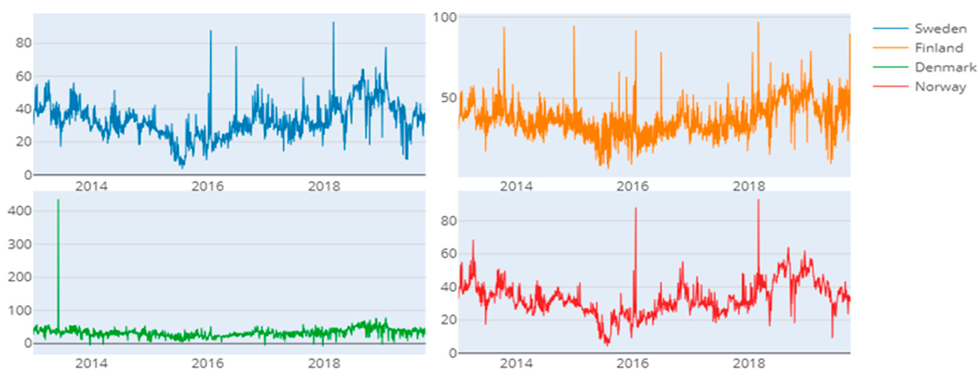
The dominant energy exchange in the Nordic power markets is called the Nord Pool. One of the first electrical markets ever established was Nord Pool. Since market participants come from 20 different nations, the market spans the majority of Europe. Different generation sources are used in the Nordic power grid. In this sector, the main sources of electricity production are hydro, nuclear, and wind energy. The energy-intensive businesses and a high proportion of electric-heated homes are in the Nordic area. Therefore, compared to the rest of the European Union (EU), this region of the world has higher electricity usage. Weather conditions have a big impact on how much electricity is consumed. For instance, summertime power consumption is lower than winter demand, which is much higher. Compared to the rest of the EU, the Nordic nations produce more clean energy. Moreover, half of the electricity generated in this area comes from hydropower. The day-ahead, intraday, and balancing markets are among the ‘time windows’ for physical energy trading in the Nordic power sector. In this zone, trading is performed mainly on the day-ahead market (spot market). The intraday and balancing markets, as well as the financial market for long-term contracts, depend on the “system price”, which is the average Nordic price for the entire following 24-h period. The intraday market is largely a corrective market, giving participants the chance to trade into balance and, if expectations prove to be inaccurate, to modify any prior trading. One hour before to delivery time, the intraday market closes. The Nordic transmission system operators (TSOs) use automatic and manual reserves, which are traded on the balancing market, to maintain power balance during the operating hour. The day-ahead and intraday markets are handled by Nord Pool Spot, and the TSOs handle the balancing market. Early in the 1990s, the Nordic nations liberalized their electricity markets and combined them into a single Nordic market. Between 2010 and 2013, Estonia, Latvia, and Lithuania liberalized their power markets and joined the Nord Pool market. The Nordic power market has grown steadily since deregulation; it now dominates the electrical markets of 13 nations. Additionally, Belgium, Germany, the Netherlands, Luxembourg, France, and the United Kingdom are all served by Nord Pool for electricity. A total of 360 enterprises from 20 different nations trade together in the Nord Pool region. In 2019, the total amount of power exchanged on the exchange was 494 TWh. Through more grid improvements and enhanced congestion management, the integration of the Nordic market to other European markets is still ongoing. The emissions trading system further aids this integration. Market liberalization and integration at the European level continue. Out of the 494 TWh traded in the Nord Pool power exchange in 2019, 401 TWh was generated in the Nordic nations of Finland, Sweden, Norway, and Denmark.

Hydropower is the primary means of generating electricity in this area. For instance, 93% of the electricity in Norway is produced from hydroelectricity. In Finland and Sweden, wind power accounts for 35% and 40% of total power output, respectively. The amount of wind energy has increased significantly over the past few years, and it is now used to create a sizeable fraction of the energy needed to meet the Nordic region’s demand. Nord Pool nations already use power generation techniques that emit zero or very little carbon dioxide (Vaissalo 2021). Notably, the Nordic power sector employs financial contracts to hedge prices and manage risk. These contracts span daily, weekly, monthly, quarterly, and annual contracts and have a maximum 10-year time frame. The system price determined by Nord Pool is regarded as the benchmark price for the Nordic financial market. For contracts in the financial power market, there is no physical delivery. Instead, depending on whether the product is a future, cash settlement occurs throughout trading and/or the delivery period, beginning on the due date of each contract.

3.2. The Data

The Nordic Power Market website provided the information for this study. Power pricing information is reported using this database on an intraday, daily, quarterly, and annual basis. Since GARCH-type models are best suited for daily frequency, we take into account daily spot prices (Cifter 2013) and Figure 1 exhibit daily spot prices. Our sample period was inclusive from 1 January 2013 to 30 November 2019.

This study makes use of daily spot pricing information for the Nordic nations of Sweden, Finland, Denmark, and Norway. As seen below, the daily log returns are calculated.

$$R_{t,n}=\ln S_t-\ln S_{t-1}$$

(1)

where $S_{t }$ is the spot price of all Nordic countries.

In all return series of energy pricing data, ARCH (1) tests for restricted heteroscedasticity and provides a strong signal of the ARCH impact. This evidence points to the applicability and use of GARCH-type.

Table 1. Descriptive Statistics of Nord Pool Electricity Prices.

	Sweden	Finland	Denmark	Norway
Mean	−0.001	−0.006	−0.001	0.001
Variance	22.363	57.109	181.8	13.519
Skewness	−0.193	−0.351	1.913	−0.197
Kurtosis	14.061	7.405	557.987	29.801
JB	20,306.060 *	5678.239 *	31,953,708.792 *	91,154.892 *
Q (10)	228.909 *	394.840 *	360.922 *	224.302 *
Q2(10)	601.378 *	292.904 *	606.240 *	646.738 *
ADF test	−57.5070 *	−57.1508 *	−52.4757 *	−70.5293 *
ARCH-LM	406.2097 *	104.1579 *	448.5787 *	148.8755 *

Note: This table displays the descriptive data for returns on electricity pricing. The Jarque–Bera test for normality, the ARCH-LM test for conditional heteroscedasticity, the Ljung–Box test for autocorrelation with ten lags applied to raw returns, and the Ljung–Box test for autocorrelation with ten lags applied to squared returns * All show rejection of the null hypothesis at the 5% level.

presents the descriptive statistics and stochastic properties of the spot return series. We find that the four Nordic countries’ average return series values are quite close to zero. When estimating daily unconditional volatility, the standard deviation is employed, and it is noticeably larger for Denmark than for other countries. Table 1 displays the negative but significant skewness that all return series, except Denmark, exhibit, which means that all returns have longer left tails and fatter tails (more unfavorable returns) than the normal distribution. Every return series has significant kurtosis. The Jarque–Bera values demonstrate how normalcy is disregarded. All return series are stationary, as shown by the Dickey–Fuller test’s significant outcomes. The Ljung–Box test statistics in 10th and 20th order are particularly significant with respect to autocorrelation in raw and squared returns series, and LB (Ljung–Box test) shows that they do not support the null hypothesis of no autocorrelation.

4. Methodology

4.1. Regime-Switching GARCH Models

We introduced regime-switching GARCH models through MSGARCH (Markov-switching GARCH) models (Ardia et al. 2018; Zhang et al. 2019). The following moment conditions result from our assumption that $y_t$ is an interesting variable at time t, has a zero mean, and lacks serial correlation: E($y_t$) = 0 and E ($y_t$ $y_{t-1}$) = 0 for t > 0 and i ≠ 0. This assumption is valid for extreme frequency returns, for which the mean (conditional) is commonly taken to be zero (McNeil et al. 2015). In subsequent applications, the MSGARCH method must be applied to a degraded time series in order to satisfy the conditional zero mean requirement. This series is added to the sample mean when the mean is constant. When there are dynamics in the conditional means of the series, the residuals of time-series algorithms like ARFIMAX (Autoregressive Fractionally Integrated Moving Average Model with Explanatory Variables) are the demeaned time series. Therefore, the MSGARCH approaches that decouple volatility estimates and mean as well as the combined methods for mean-variance switching (Kim and Nelson 1999) are not practical. In the process for (conditional) variance, we allow regime change. Denote through ${\mathrm{H}}_{t-1}$ the info set examined up to time-period t − 1, i.e., ${\mathrm{H}}_{t-1}\equiv \left\{y_i, i>0\right\}.$The general MSGARCH condition can then be written as:

$$y_t\left|\right({\hslash }_t=l, {\mathrm{H}}_{t-1})~D \left(0, {\mathrm{N}}_{k,t}, {\mathsf{{\rm Y}}}_k\right)$$

(2)

where $D \left(0, {\mathrm{N}}_{k,t}, {\mathsf{{\rm Y}}}_k\right)$is a constant distribution with mean zero, variance ${\mathrm{N}}_{k,t}$ which is time-varying and supplementary shape parameters assembled in the vector ${\mathsf{{\rm Y}}}_k.$1 The stochastic variable of integer-valued $h_t$, explained on the distinct space {1, …, k}, exemplifies the MSGARCH method. We express the consistent innovation as:

$${\lambda }_{k,t}\equiv y_t/{\mathrm{N}}_{k,t}^{1/2} \begin{array}{c}iid\\ ~\end{array} D \left(0, 1, {\mathsf{{\rm Y}}}_k\right)$$

(3)

4.2. State Dynamic

The MSGARCH model implements two approaches to the dynamic of the state variable: the first is the assumption of a first-order ergodic, homogeneous Markov chain, which describes the MSGARCH models of (Haas et al. 2004a), and the second is the assumption of self-determining draws as a multinomial distribution, which describes the Combination of GARCH approaches of (Haas et al. 2004b). Therefore, we mainly concentrate on the first premise that characterizes MSGARCH models. We suppose that $h_t$ evolves conferring to an ignored 1st order ergodic homogenous-Markov chain with K × K conversion probability-matrix R:

$$R\equiv \left[\begin{array}{ccc}r \mathrm{1,1}& \cdots & r1, k\\ ⋮& \ddots & ⋮\\ rk,1& \cdots & rk, k \end{array}\right]$$

(4)

where $r_{i,j}\equiv R[{\mathrm{\hslash }}_t=j|{\mathrm{\hslash }}_{t-1}=i]$ is the probability of a conversion from state ${\mathrm{\hslash }}_{t-1}=i$ to state ${\mathrm{\hslash }}_t=j$. Apparently, the next constraint hold: $0<r_{i,j}<1\forall i,jϵ\left\{1,\dots \dots ,K\right\}$ and $\sum _{j=1}^k{r}_{i,j}=1,\forall iϵ\left\{1,\dots ..,K\right\}.$ Assumed the parametrization of D(.), we achieve $E\left[y_t^2|{\mathrm{\hslash }}_t=k,{\mathfrak{h}}_{t-1},\right]={\mathrm{N}}_{k,t},$ i.e., ${\mathrm{N}}_{k,t}$ is the variance of y_t uncertain on the recognition of ${\mathrm{\hslash }}_t=k$. The variance (conditional) ${\mathrm{N}}_{k,t}$ for k = 1 … K are given to follow K different GARCH type process that evolves in equivalent in the MAGARCH method of (Haas et al. 2004a).

4.3. Conditional-Variance Dynamics

The conditional variance of $y_t$ is expected to follow a GARCH-type technique, according to (Haas et al. 2004a). The last observation, y_t−1 previous variance, ${\mathrm{N}}_{k,t-1}$, and the additional regime-dependent parameter vectors ${\mathcal{v}}_k$ are supplied, confined to the regime ${\hslash }_t=k, {\mathrm{N}}_{k,t}$.

$${\mathrm{N}}_{k,t}=\hslash \left(y_{t-1},{\mathrm{N}}_{k, t-1},{\mathcal{v}}_k\right),$$

(5)

where ν (.) is a ${\mathfrak{h}}_{t-1}$ an obtainable function that explains the filter for the conditional variance and confirms its positivity as well. In the MSGARCH method, the first value of the variance persistent, i.e.,${\mathrm{N}}_{k,1}\left(k=1,\dots ..,K\right)$ are established equivalent to the unconditional variance in the k regime. We get different scedastic conditions depending on the case of ν (.). Lastly, when K = 1, we obtain single-regime GARCH-type methods identified through the form of ν (.). (Engle 1982) introduced the ARCH model, which is given by:

$${\mathrm{N}}_{k,t}={\mathrm{A}}_{0,k}+{\mathrm{A}}_{1,k}{y}_{t-1}^2,$$

(6)

For k = 1, …, K. We have ${\mathcal{v}}_k=({\mathrm{A}}_{0,k},{\mathrm{A}}_{1,k}{)}^T$ in this case. To confirm positivity, we need that ${\mathrm{A}}_{0,k}>0$, ${\mathrm{A}}_{1,k}\ge 0$ as well. Co-variance stationarity is every regime is measured by demanding that ${\mathrm{A}}_{1,k}<1.$ The ARCH condition is acknowledged with the name “sARCH”.

(Bollerslev 1986) explained the GARCH model as:

$${\mathrm{N}}_{k,t}={\mathrm{A}}_{0,k}+{\mathrm{A}}_{1,k}{y}_{t-1}^2+{\mathrm{B}}_k{\mathrm{N}}_{k,t-1},$$

(7)

For k = 1, ..., K. we have ${\mathcal{v}}_k=({\mathrm{A}}_{0,k},{\mathrm{A}}_{1,k},{\mathrm{B}}_k{)}^T$ in this case. To confirm positivity, we need that ${\mathrm{A}}_{0,k}>0$, ${\mathrm{A}}_{1,k}\ge 0, {\mathrm{B}}_k\ge 0$ as well. Co-variance stationarity in every regime is measured by demanding that ${\mathrm{A}}_{1,k}+{\mathrm{B}}_k<1.$ The GARCH condition is acknowledged as “sGARCH”.

(Nelson 1991) presented the EGARCH (Exponential GARCH) model, given as:

$$\ln \left({\mathrm{N}}_{k,t}\right)\equiv {\mathrm{A}}_{0,k}+{\mathrm{A}}_{1,k}\left(\left|{\varphi }_{k,t-1}\right|-E\left[\left|{\varphi }_{k,t-1}\right|\right]\right)+{\mathrm{A}}_{2,k}{y}_{t-1}+{\mathrm{B}}_k\ln \left({\mathrm{N}}_{k,t-1}\right),$$

(8)

For k = 1, ..., K, where the expectancy $E\left[\left|{\varphi }_{k,t-1}\right|\right]$ is occupied with respect to the distribution restricted on the k regime. We have ${\mathcal{v}}_k=({\mathrm{A}}_{0,k},{\mathrm{A}}_{1,k},{\mathrm{A}}_{2,k},{\mathrm{B}}_k{)}^T$ in this case. This condition considers the so-called “leverage effect” where previous adverse observations have a huge influence on the restricted volatility that previous positive observations of a similar degree (Dhingra et al. 2024; Christie 1982). Positivity is repeatedly confirmed through the model condition. Co-variance stationarity in every regime is measured by demanding that ${\beta }_k<1$. The EGARCH condition is acknowledged as “eGARCH”. The GJR model is introduced by (Glosten et al. 1993) which can obtain the asymmetry in the restricted volatility procedure. This model is explained as:

$${\mathrm{N}}_{k,t}\equiv {\mathrm{A}}_{0,k}+\left({\mathrm{A}}_{1,k}+{\mathrm{A}}_{2,k}\mathbb{J}\left\{y_{t-1}<0\right\}\right)y_{t-1}^2+{\mathrm{B}}_k{\mathrm{N}}_{k,t-1},$$

(9)

For k = 1, …, K where $\mathbb{J}\left\{.\right\}$is the pointer function having value 1 if the specification holds, or else zero. We have ${\mathcal{v}}_k=({\mathrm{A}}_{0,k},{\mathrm{A}}_{1,k},{\mathrm{A}}_{2,k},{\mathrm{B}}_k{)}^T$ in this case. The parameter ${\mathrm{A}}_{2,k}$ regulates the magnitude of asymmetry in the restricted volatility reaction to the previous shock in the k regime. To confirm positivity, we need that ${\mathrm{A}}_{0,k}>0, {\mathrm{A}}_{1,k}>0, {\mathrm{A}}_{2,k}\ge 0, \mathrm{a}\mathrm{n}\mathrm{d} {\mathrm{B}}_k\ge 0.$ Co-variance stationarity in every regime is measured by demanding that ${\mathrm{A}}_{0,k}+{\mathrm{A}}_{2,k}E\left[{\varphi }_{k,t}^2\mathbb{J}\left\{{\varphi }_{k,t}<0\right\}\right]+{\mathrm{B}}_k<1$. The GJR condition is explained as “gjrGARCH”.

4.4. Conditional Distribution

Specification of the model is finalized through the description of the conditional distribution of the standardized inventions ${\varphi }_{t,k}$ in every regime of the Markov chain. The most usual distributions implemented to model monetary log returns are employed. Every distribution is consistent to have a zero mean and unit variance. By way of the conditional-variance condition, distributions are acknowledged with names. In this case, we drop the regime indices and time for notational determinations, nevertheless, the shape parameters can be restricted on the regime.

4.4.1. Normal Distribution

The PDF (probability density function) of the traditional normal distribution is explained as:

$$f_N\left(\mathrm{X}\right)\equiv {\displaystyle \frac{1}{\sqrt{2\pi }}}{e}^{-{\displaystyle \frac{1}{2}}{\mathrm{X}}^2}, \mathrm{X} ϵ \mathbb{R}.$$

(10)

This distribution is acknowledged as “norm”.

4.4.2. Model Computation

Computation of MSGARCH methods can be completed through ML procedures. The procedures need the estimation of the probability function. Let $\mathsf{\Omega }\equiv ({\mathcal{v}}_1,{\mathsf{\Psi }}_1,\dots ..,{\mathcal{v}}_K,{\mathsf{\Psi }}_K,R)$ be the model-parameters vector. The probability function is:

$$j(\mathsf{\Omega }\left|{\mathrm{H}}_T)\equiv \prod _{t=1}^{T}f{(y}_t\right|\mathsf{\Omega }, {\mathrm{H}}_{t-1}),$$

(11)

where, $f\left(y_t|\mathsf{\Omega }, {\mathrm{H}}_{t-1}\right)$ referred to the density of y_t providing previous observation, ${\mathrm{H}}_{t-1},$and a parameter of model $\mathsf{\Omega }.$ The restricted density of $y_t$ for MSGARCH is:

$$f\left(y_t|\mathsf{\Omega }, {\mathrm{H}}_{t-1}\right)\equiv \sum _{i=1}^K\sum _{j=1}^K{r}_{i,j},z_{i,t-1}{f}_D\left(y_t|{\hslash }_t=j, \mathsf{\Omega }, {\mathrm{H}}_{t-1}\right),$$

(12)

where, $z_{i,t-1}\equiv R[{\hslash }_{t-1}=i|\mathsf{\Omega },{\mathrm{H}}_{t-1}]$ explained the filtered likelihood of state $i$ at period $t-1$ measured by the filter of Hamilton; for details (Hamilton 1989, 1994). The estimator of ML $\mathsf{\Omega }$ is measured by maximizing the log of Equation (3)2.

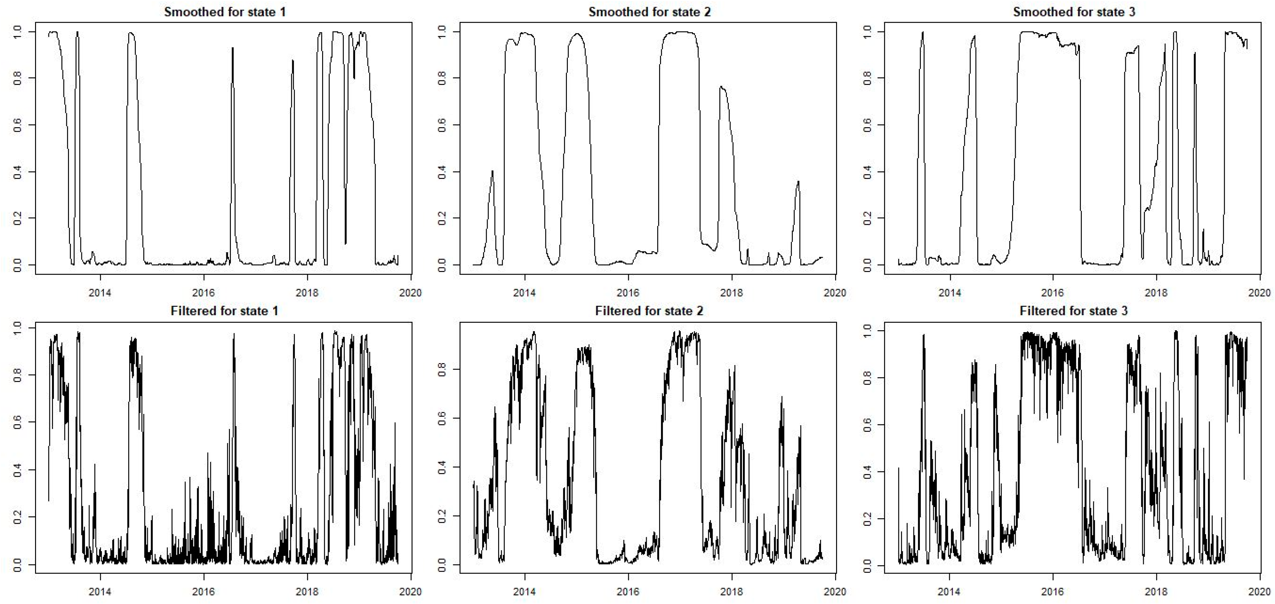
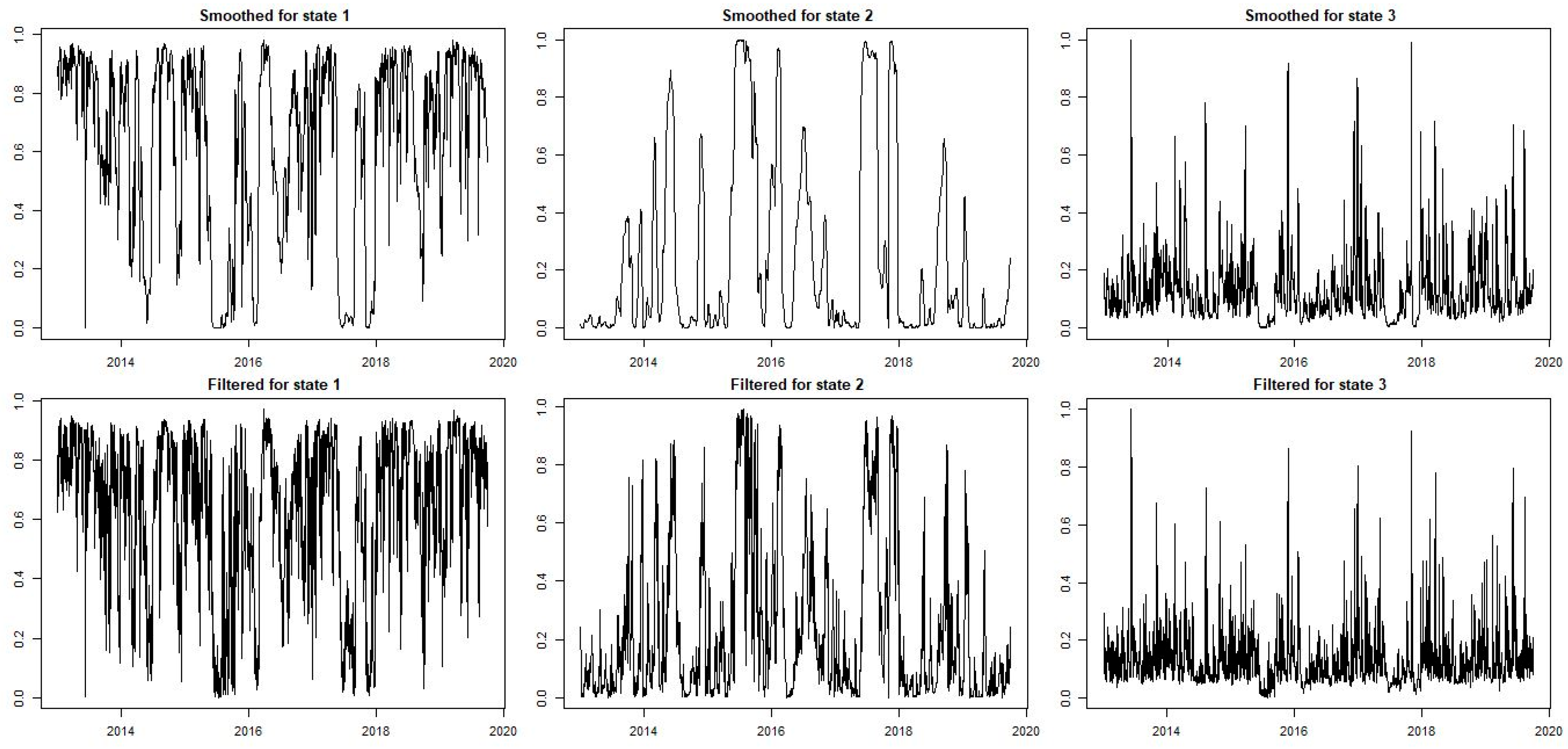
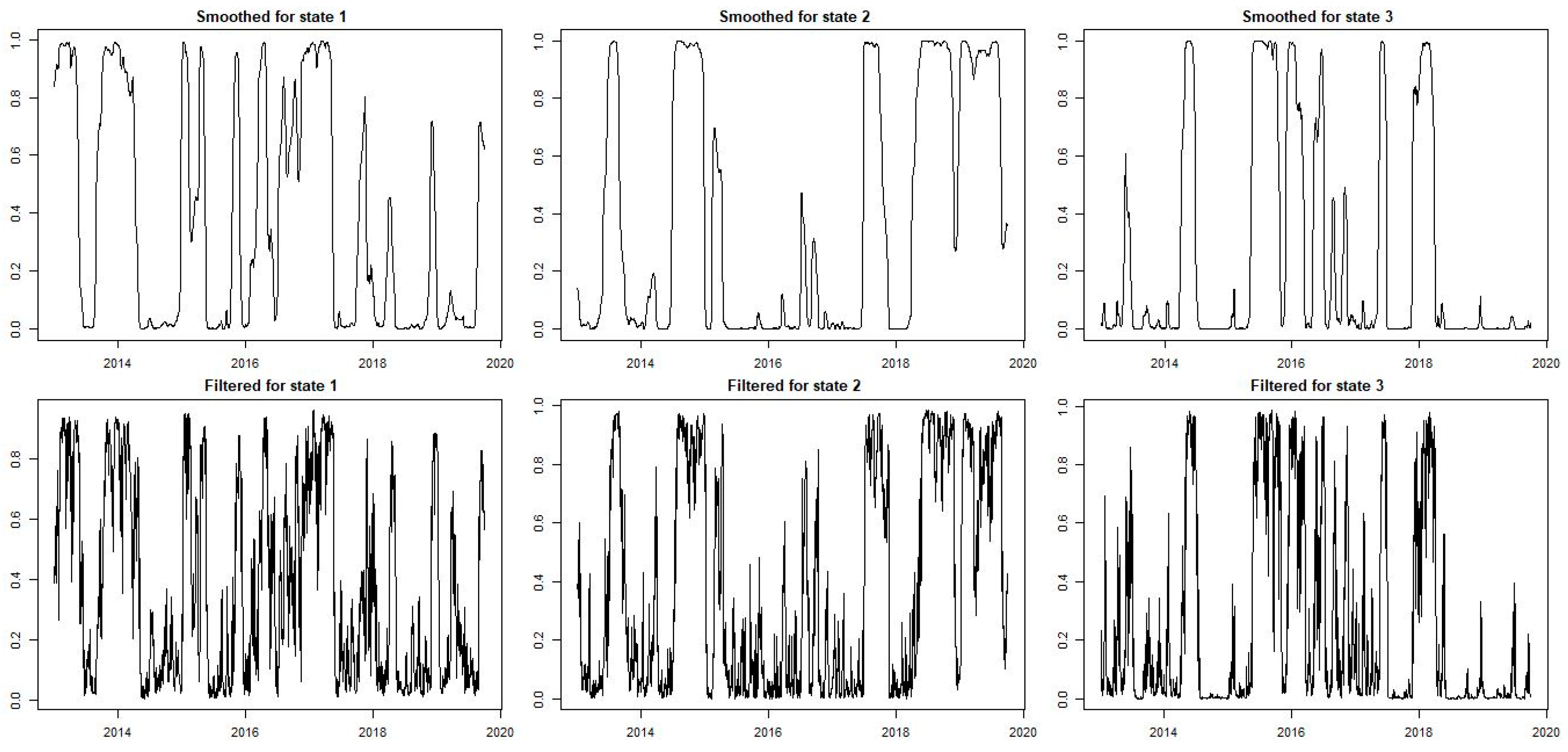
5. Empirical Findings

With differing degrees of parameter stipulations, we empirically determine the estimates for regime-switching GARCH techniques and incorporate variables to represent the volatility in various regimes. AIC is the best metric to use when choosing a model. The best model is GJR-GARCH (regime = 3) with the student-t distribution. All four models for series are computed with and without nonlinearity in the mean equations. The results unmistakably demonstrate that all models with nonlinearity effects have more interpersonal dynamics than ones without. Simply put, we report estimation in nonlinear instances. With the estimates from the most recent literature, this is trustworthy. The probability of the system being in a specific regime is tracked over time in the MSGARCH model using smooth and filtered probabilities. While the filtered probabilities are determined using only the data up to a specific point in time, the smooth probabilities are calculated utilizing all the available data. The smooth and filtered probability will behave differently in various regimes. The smooth probability will be comparatively high for that regime, for instance, if the system is now in a low-volatility regime. The filtered probability, however, might be lower since they did not account for all the information pointing to the system being in a low-volatility regime. As the model gains additional data, the filtered probabilities will eventually converge to the smooth probabilities. The filtered probabilities, however, will always be based only on a portion of the available data. Thus, there will always be some discrepancy between the two. The probabilities that have been smoothed and filtered can be used to track the system’s development and forecast the future. For instance, a system may be going toward a low-volatility state (regime) if the smooth probability for a low-volatility regime is rising.

The computed parameters for MSGARCH models are listed in

Table 2. Modeling Volatilities of Nord Pool Electricity Prices by using MSGARCH.

Countries	Sweden	Finland	Denmark	Norway
Models	GJR-GARCH	GJR-GARCH	GJR-GARCH	GJR-GARCH
	(regime = 3)	(regime = 3)	(regime = 3)	(regime = 3)
Distribution	std-std-std	std-std-std	std-std-std	std-std-std
Parameters
Regime 1
α0–1	4.967	56.1902	15.2273	38.608
	(2.1194)	(16.398)	(11.1783)	(10.3523)
α1–1	0.0229	0.0003	0.0057	0.3354 *
	(0.018)	(0.0022)	(0.0147)	(0.1424)
α2–1	0.0004	0.2394	0.1983	0.0002
	(0.003)	(0.153)	(0.2358)	(0.0032)
β−1	0.9341 *	0.3985 *	0.8908 *	0.2058 *
	(0.0157)	(0.1345)	(0.012)	(0.1372)
ν−1	9.7953 *	4.2092 *	11.0146 *	3.7899 *
	(4.5887)	(0.9195)	(6.6024)	(0.7265)
Regime 2
α0–2	24.7002	2.9905	271.4789	10.7384
	(5.4427)	(2.3036)	(65.0001)	(2.4515)
α1–2	0.0003	0.0002	0.0007	0
	(0.0161)	(0.0049)	(0.006)	(0.0007)
α2–2	1.2908 *	0.0228	1.666 *	1.155 *
	(0.1933)	(0.0171)	(0.1024)	(0.3097)
β−2	0.2565 *	0.9794 *	0.1065 *	0.3785 *
	(0.0884)	(0.0082)	(0.052)	(0.0825)
ν−2	3.6721 *	4.3517 *	3.0817 *	3.717 *
	(0.5427)	(0.7954)	(0.323)	(0.5421)
Regime 3
α0–3	54.416	106.3726	24,841.56	107.0368
	(29.3901)	(58.0858)	(21,319.97)	(57.087)
α1–3	0.0001	0	0.0595	0.195
	(0.0021)	(0.000)	(0.4527)	(0.1254)
α2–3	0.1531	0.3466 *	0.0007	0.0849
	(0.2441)	(0.1841)	(0.0043)	(0.152)
β−3	0.9214 *	0.7573 *	0.0016	0.452 *
	(0.006)	(0.0545)	(0.0103)	(0.1626)
ν−3	99.9112 *	3.9358 *	73.042	4.4527 *
	(1.2583)	(0.6558)	(416.7)	(0.9248)
Probabilities
ρ−1–1	0.9245	0.9865	0.974	0.986
	(0.4144)	(0.000)	(0.0091)	(0.0183)
ρ−1–2	0.0345	0.007	0.0249	0.0032
	(0.1012)	(0.0062)	(0.3973)	(0.0052)
ρ−2–1	0.0299	0	0.0089	0.0086
	(0.0236)	(0.0487)	(0.0423)	(0.0033)
ρ−2–2	0.9615	0.9936	0.9827	0.9913
	(0.000)	(0.000)	(0.3201)	(0.0995)
ρ−3–1	0.2813	0.009	0.0942	0.0095
	(0.0216)	(0.0448)	(0.0007)	(0.0063)
ρ−3–2	0	0	0.6105	0.0085
	(0.1187)	(0.0444)	(0.0071)	(0.000)
ρ−3–3	0.7187	0.9910	0.2953	0.9819
AIC	18,971.47	21,160.01	22,325.9007	17,421.9354
BIC	19,093.47	21,281.99	22,447.8926	17,543.9273
LL	−9464.73	−10,559.00	−11,141.9504	−8689.9677

Note: Standard errors are in parenthesis. * indicate significance at 5%.

. According to our findings, the conditional variance parameters are significant for all return series. The parameters estimate for the Nord Pool power price series supports three regimes. The first and third regimes for Sweden are categorized as having minimal volatility. However, the second regime has a higher level of volatility than the other two regimes. Furthermore, regime 1 is more unstable for Finland than the other two. Furthermore, regime 3 is more volatile for Denmark and Norway compared to the other two regimes.

The importance of the characteristics shows that Nordic electricity prices were volatile and persistent across all regimes. Additionally, because most distribution-specific properties are important, the selection of distributions is suitable. The Markov chain transition probability reveals how the price dynamics of electricity prices change between regimes. Apart from Denmark, where there is a 61% chance of moving from state 3 (regime 3) to state 2 (regime 2), we note that the likelihood of changing states is relatively low and the likelihood of remaining in the same state (regime) is relatively high. This shows that there is minimal possibility of a process-changing state (regime) while it is under a single regime, except in Denmark. The probabilities for remaining within the state are $p_{11}$, $p_{22}$ and $p_{33}$ while moving from one state (regime) to another is denoted by $p_{12}$, $p_{21}$, $p_{31}$, $p_{13}$, $p_{32}$, and $p_{23}$. The results show that Markov-switching GARCH models are more capable of identifying and differentiating between distinct sources of volatility clustering. Persistence within regimes and regime persistence are the two types of volatility clustering that (Gray 1996) describes. Since the regimes are persistent, it follows that whenever a high-volatility regime occurs, the high-volatility phases likely cluster if the unconditional variance in one regime is more significant than in the others. This demonstrates how the persistence of the high volatility regime causes volatility clustering in any regime for electricity price returns. Additionally, persistence within and between regimes impacts how volatility clusters. The AIC offers a fundamental understanding of whether regime persistence significantly contributes to volatility clustering. The AIC for regime-switching models is lower than that of single-regime models for each model specification with a different error distribution. Consequently, connected regimes are a vital channel for capturing volatility clustering.

The GJR-GARCH (1,1,1) model with conditional student-t distribution in all three of the regimes shown in Table 2 was the most successfully chosen for Sweden. All three regimes’ extremely significant parameters ensure that conditional volatility is positive, that all are bigger than zero, and that there is covariance stationarity. The volatility parameter α_{1, k} shows lower unconditional volatility for all regimes since the parameter does not seem to be significant. We observe a leverage effect in regime 2. All the regimes are highly persistent, with posterior probabilities $p_{11}$, $p_{22}$ and $p_{33}$ at 92%, 96%, and 72%, respectively. The variance parameter β_-k ranges from 0.2565 to 0.9341 showing high volatility in the first and third regimes but lower volatility observed in regime 2 compared to regimes 1 and 3. The degree of freedom is greater than two, which suggests that the second-order moment is present. The best model is picked based on the lowest AIC, −9464.73. For the Sweden instance of the GJR-GARCH (1,1,1), Figure 2 shows the estimated smoothed probabilities and filtered conditional volatilities. To extract filtered volatility from calculated objects, use the volatility function. The first and second regimes have significant, smoothed probability, and the filtered volatility technique advances swiftly, as can be seen from the results. The reported probabilities in the first and second states (regimes) are 48% and 43%, respectively, much higher than the probabilities in state (regime) three, i.e., 9%. Surprisingly, we discovered that the Markov chain evolves deterministically over time. The parameter α_{1, k} is insignificant for all regimes, depicting the lowest unconditional volatility. The leverage parameter α_{2, k} ranges from 0.0228 to 0.3466 in all regimes, but the impact is statistically weak. The variance parameter β₋₁ for regime 1, β₋₂ for regime 2, and β₋₃ for regime 3 are significant and depict 40%, 98%, and 76% volatility, respectively, showing the volatility procedure’s high determination.

Furthermore, the degree of freedom is greater than two, indicating the existence of a second-conditional moment. Due to the transition probabilities being close to one, which suggests that almost all regimes are persistent, the probabilities are highly relevant for all regimes. All regimes’ significant degree of flexibility demonstrates that distributions have thicker tails. Based on the lowest AIC value, −24,780.48, the optimal model for silver is chosen. Figure 3 displays the calculated smoothed probabilities and filtered conditional volatilities for the Finland example of the GJR-GARCH (1,1,1). The smoothed probabilities for the first two states in the results are 28% and 30%, respectively. More importantly, we observed that the Markov chain evolves purposefully over time, the filtered volatility of the procedure is rapidly increasing, and the reported probability in the third state is 42%, which is higher than the reported probabilities in states 1 and 2. The GJR-GARCH (1,1,1) with student-t distributions model is the one that works the best for Denmark, and the constant is both significant and positive. As a non-significant parameter, the parameter 1, k exhibits modest unconditional volatility for all regimes.

The variance parameter β₋₁ shows high persistence volatility, while on the other hand, parameters β₋₂ and β₋₃ weak volatility is observed in regimes 2 and 3, respectively. The leverage parameter α_{2, k} ranges from 0.007 to 1.66 upon which regime 2 shows leverage impact is present there. All the regimes are highly persistent, with posterior probabilities $p_{11}$, $p_{22}$ $p_{23}$, and $p_{33}$ at 97%, 98%, 61%, and 29%, respectively. The degree-of-freedoms are more significant across all regimes, showing the distributions have thicker tails. The model selection is based on the 22,325.9 AIC value.

Figure 4 displays the calculated smoothed probabilities and filtered conditional volatilities for the Denmark instance of the GJR-GARCH (1,1,1). The smoothed probability of the two states is almost one, as seen in the results, with the filtered probabilities of the procedure increasing quickly in both regimes. We were increasingly aware of the Markov chain’s deterministic evolution through time and its approximately 28%, 71%, and 0.08% odds of being in each state, respectively. Parameter estimations demonstrate that the volatility procedure’s development is uneven across the three regimes. All three regimes exhibited varying levels of unconditional volatility, as we noticed. In regime 1, parameter α_{1, 1} shows a low unconditional volatility of 33%; the remaining parameters of unconditional volatilities are insignificant. The leverage parameter α_2,k ranges from 0.0002 to 1.155, upon which regimes 2 and 3 show leverage effect exists. The variance parameters β₋₁ for regime 1, β₋₂ for regime 2, and β₋₃ for regime 3 are significant and depict 20%, 38%, and 45% volatility, respectively, showing the volatility procedure’s high determination. Due to the transition probabilities being close to one, which indicates that almost all regimes are persistent, the probabilities are highly relevant for all regimes. All regimes’ significant degree of flexibility demonstrates that distributions have thicker tails. The lowest AIC value, or 17,421.93, is used to determine the optimal model for Norway.

Figure 5 displays the calculated smoothed probability and filtered conditional volatilities for the instance of Norway using the GJR-GARCH (1,1,1). As we saw in the findings, the filtered probabilities of the operation in regime 1 are fast-growing, while the smoothed probability of state 1 is close to one. We were more aware of the Markov chain’s deterministic evolution through time and its approximately 39%, 37%, and 23% odds of existing in each state (regime).

At first, we thought about performing an in-sample study to fit the multiple models to the entire data set. We demean the series and remove autoregressive effects from the data using an AR (1) filter because we are interested in volatility dynamics, and then we estimate the models on the residuals. We employ the AIC to assess the models’ goodness-of-fit. The AIC is just meant to compare a variety of possible formulations and choose the most suitable one. It is not meant to identify the proper model. In contrast to their single-regime counterparts, the three-regime MSGARCH models offer a better trade-off between model complexity and fitting quality for all volatility and distribution criteria. We also point out that fat-tailed and skewed distributions are favored for all regime specifications. We now look at Table 2 parameter estimates for the top in-sample models for all return series.

We now assess the capability of regime-switching models to accurately predict Value-at-Risk (VaR) one day in advance using an out-of-sample approach. For rolling window in-sample estimation, we use data from 1 January 2013 to 1 March 2017, totaling 1463 observations. We do the back-test using 1000 out-of-sample data for the time span between 1 April 2017 and 30 September 2019. We employ the Conditional Coverage Test of (Christoffersen 1998) and the Dynamic Quantile Test (DQ) of (Engle and Manganelli 2004) to assess the suitability of each model. The following publication (Ardia et al. 2018) provides more details regarding these tests about Value-at-Risk calculations. We derive the p-values for the UC and DQ tests computed using 1000 out-of-sample observations for the best models. A suitable model for predicting Value-at-Risk should provide an accurate percentage of breaches of Value-at-Risk and information about how these violations vary over time.

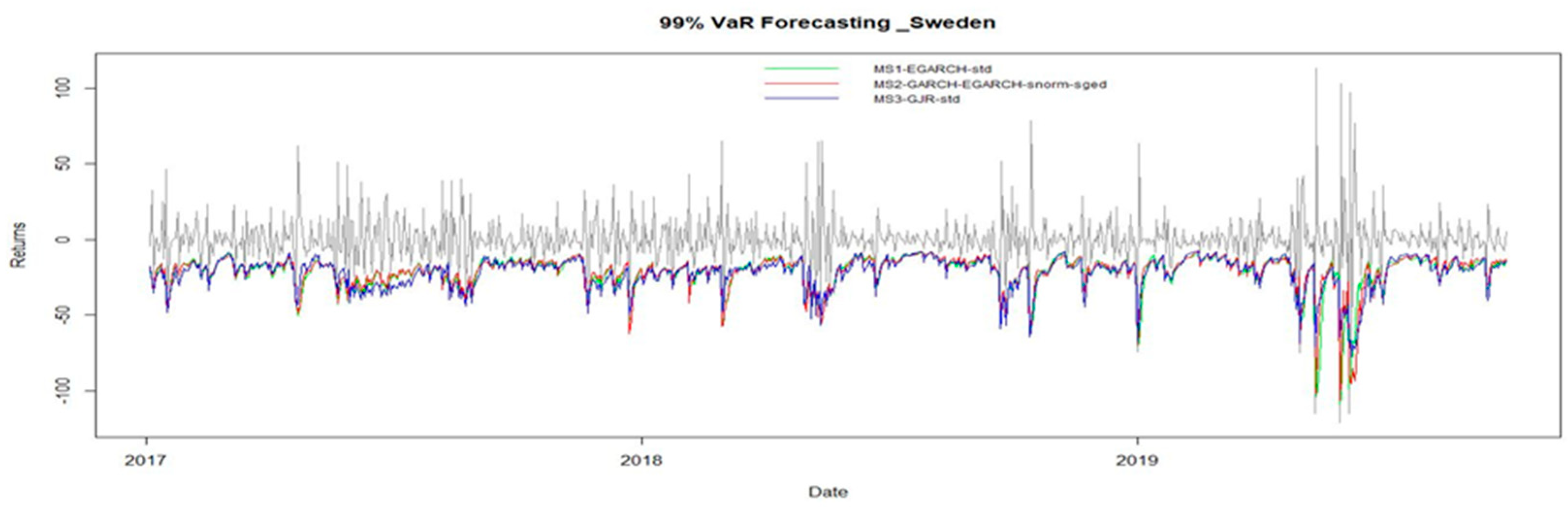
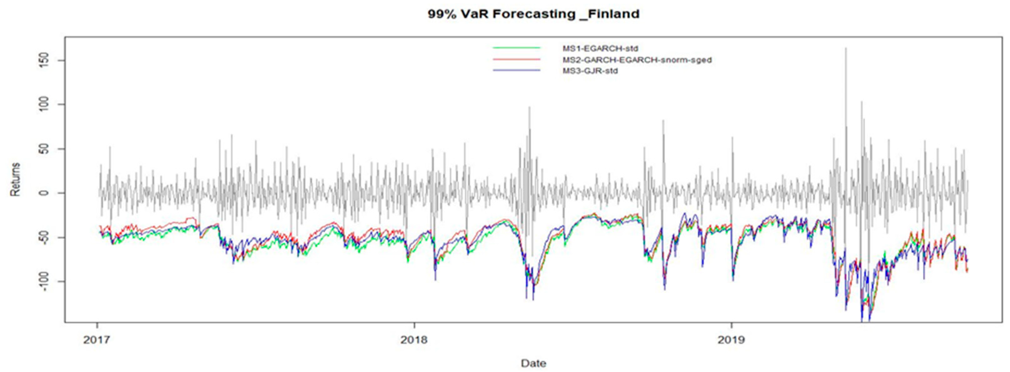
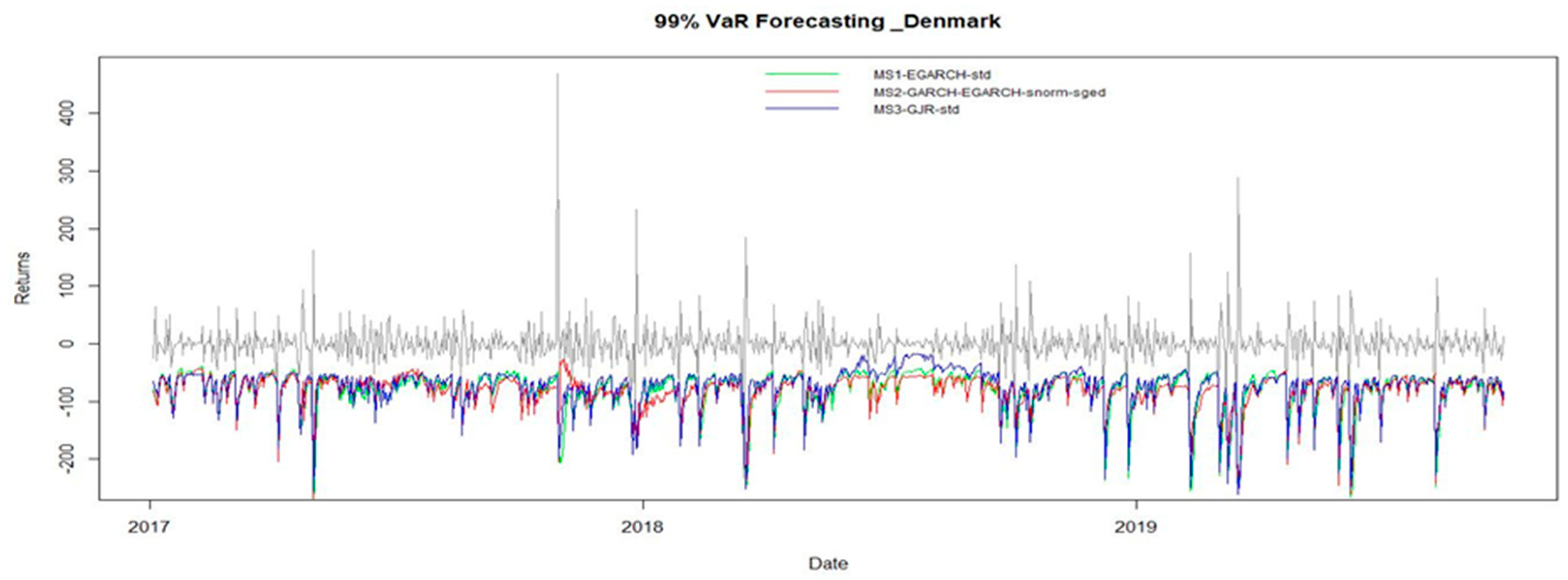
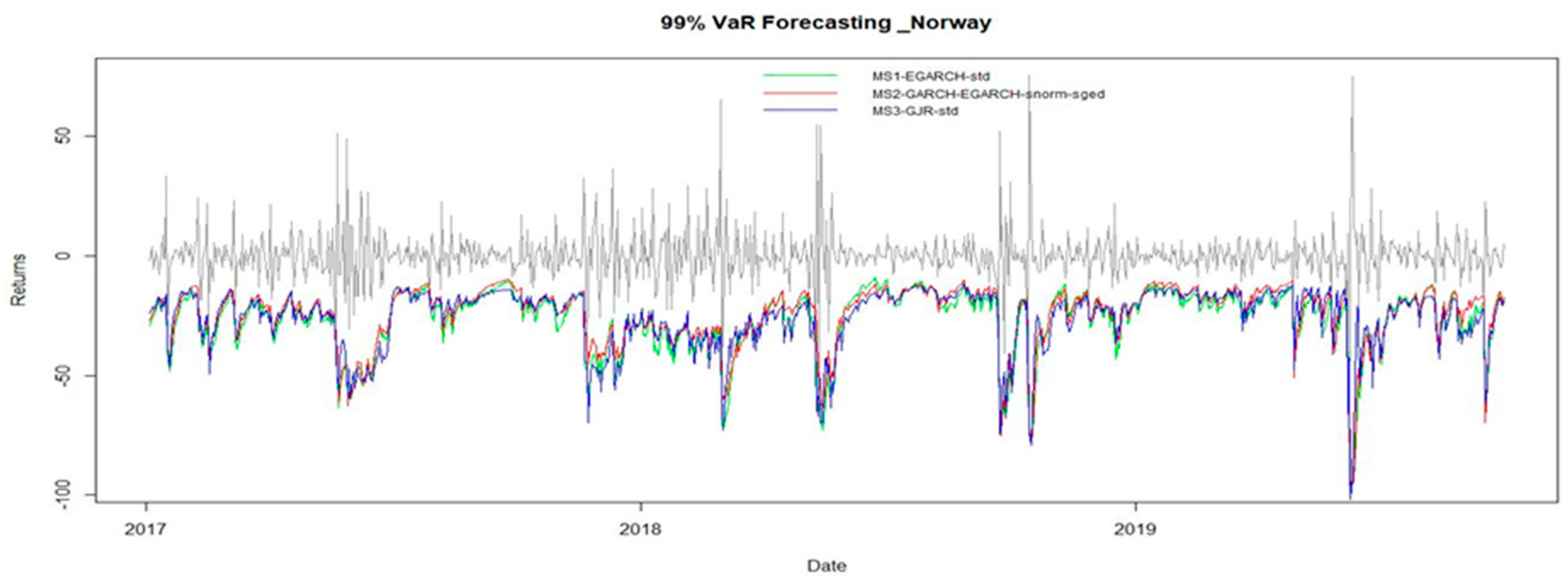
Insights from Value-at-Risk Analysis

Table 3. Value-at-Risk Calculations and 1% and 5% level.

Test	CC Test				DQ Test
Country	Sweden	Finland	Denmark	Norway	Sweden	Finland	Denmark	Norway
Var 1%
Regime 1	0.84	0.39	0.006	0.17	0.99	0.92	0.26	0.003
Regime 2	0.16	0.05	0.003	0.02	0.84	0.34	0.079	0.00
Regime 3	0.71	0.15	0.003	0.17	0.92	0.78	0.067	0.002
Var 5%
Regime 1	0.83	0.36	0.94	0.04	0.75	0.34	0.998	0.14
Regime 2	0.85	0.33	0.28	0.07	0.81	0.25	0.995	0.09
Regime 3	0.67	0.44	0.60	0.26	0.69	0.49	0.999	0.04

Note: The conditional coverage test (CC) and dynamic quantile test (DQ) p-values at 1% and 5% for the one-day ahead Value-at-Risk forecast are shown in the table. We emphasize p-values above 5% in bold.

displays the one-day ahead Value-at-Risk p-values for the CC and DQ tests, which have 1% and 5% risk levels, respectively. We found that, at the 5% level, the multiple regime-switching specification accurately predicted the Value-at-Risk. Therefore, in most cases, the assumption of accurate Value-at-Risk forecasting for multiple regimes MSGARCH models at both the 1% and 5% levels must be addressed. The Value-at-Risk value behavior for all Nordic power prices at the 1% level is also shown in Figure 6, Figure 7, Figure 8 and Figure 9.

6. Conclusions and Policy Implications

The deregulation trend that is revolutionizing the electrical business globally is causing electrical costs to be substantially more volatile than the pricing of other commodities. However, industry and economic development both depend heavily on power. So, the power market could affect the stock market by changing real output and, consequently, the total cash flows. Because of the risks related to the electricity market, investors must devise methods to protect their gains. In this research, we investigate the problem of creating a framework for risk management and hedging strategies in the Nordic market. We investigated regime-switching models to capture electricity spot price events to accomplish this. The characteristics of regime switching in the volatility of the Nord Pool electricity spot prices for Sweden, Finland, Denmark, and Norway are examined in this research. As a result, we demonstrate that the volatility dynamics of Nord pool daily log-returns display regime changes using Markov-switching GARCH models, which are specifications that may take into account structural breaks in GARCH. To evaluate the in-sample analysis of volatility, we fitted a variety of single and multiple regime models to the log returns of each electricity spot price. We compare models using the Akaike information criterion (AIC) for all electrical spot price returns series and select the top models in each regime. Furthermore, the chosen models are used in comparing classic single-regime GARCH models with regime-switching GARCH models for forecasting one-day ahead Value-at-Risk. As a result, the findings of the in-sample analysis demonstrate that regime-switching models consistently outperform their single-regime counterparts. However, the findings of the out-of-sample investigation indicate that the GARCH process is subject to regime changes and show that when estimating the Value-at-Risk for this electricity, regime-switching GARCH models perform better than single-regime GARCH specifications. The regime-switching aspect in the volatility of electricity spot price returns is very important because Value-at-Risk prediction is crucial for risk management and appropriate portfolio allocations. As a result, our results for both in-sample and out-of-sample research point to the fact that including regime-switching in volatility modeling is suitable for risk management related to the price dynamics of electricity prices (but not all) in general.

6.1. Discussion

Our findings related to in-sample analysis and out-of-sample forecasting are consistent with the results of (Zhang et al. 2019). It is crucial to highlight that the bulk of studies emphasize the value of risk management for the decision-making processes employed in the power markets. Understanding the market’s structure and having power pricing models that forecast the market’s future behavior is essential for selecting the appropriate hedging strategy. It is found that by employing hedging tactics that have been effective in the financial and other commodity markets, electricity futures may effectively control risk only for specific time periods. Several instruments are suggested in this context, including forward, bilateral, and futures contracts (Andriosopoulos and Nomikos 2013). Correct VaR computation is essential for all market players in the volatile energy markets for various reasons. Managers can use it to design sensible hedging strategies to protect their investments. Second, the suggested VaR model selection process minimizes modeling risk while meeting strict risk management criteria and control processes by decreasing the possibility of accepting substandard models. Third, many hedge fund managers and alternative investors who have just started paying close attention to and expanding their presence in the energy markets believe that it is crucial to evaluate the risk profile of the energy markets. Last but not least, (Londoño and Velásquez 2023) found that, even though risk management did not prevent a decline in investment portfolios during the recent economic recession, those organizations that had made investments in risk management procedures before the crisis and taken action on their findings performed significantly better than those that did not support the value of good risk management procedures.

6.2. Limitations and Future Research

There are some limitations to this study. It is limited to the Nordic electricity market, which limits the applicability of results to other places or markets. Yet regime-switching GARCH models can capture structural breaks but not necessarily exogenous shocks such as geopolitics or extreme weather. There is also limited analysis on hedging strategies and no attempts to examine whether these strategies can be adapted under different market environments or for different time horizons. In addition, out-of-sample forecasting performance differs across electricity price series, and the potential effects of greater interconnections to other financial or commodity markets are ignored. Future studies could fill these gaps by the application of the proposed methodology to the other electricity markets, integrating external elements such as those reflected in renewable energy and geopolitical risks, as well as investigating interrelationships with other financial or commodity markets. Further improving prediction accuracy might come from trying different modeling techniques like stochastic volatility or machine learning-based approaches. Practical insights would also be derived by devising adaptive hedging strategies and evaluating model performance over different time horizons.

References

1. Andriosopoulos, Kostas, and Nikos Nomikos. 2013. Risk management in the energy markets and Value-at-Risk modelling: A hybrid approach. The European Journal of Finance 21: 548–74. [Google Scholar] [CrossRef]
2. Ardia, David, Keven Bluteau, Kris Boudt, and Leopoldo Catania. 2018. Forecasting risk with Markov-switching GARCH models: A large-scale performance study. International Journal of Forecasting 34: 733–47. [Google Scholar] [CrossRef]
3. Ardia, David, Keven Bluteau, Kris Boudt, Leopoldo Catania, and Denis-Alexandre Trottier. 2019. Markov-switching GARCH models in R: The MSGARCH package. Journal of Statistical Software 91: 1–38. [Google Scholar] [CrossRef]
4. Amaro, Raphael, Carlos Pinho, and Mara Madaleno. 2022. Forecasting the Value-at-Risk of energy commodities: A comparison of models and alternative distribution functions. Applied Econometrics 65: 77–101. [Google Scholar] [CrossRef]
5. Bollerslev, Tim. 1986. Generalized autoregressive conditional heteroskedasticity. Journal of Econometrics 31: 307–27. [Google Scholar] [CrossRef]
6. Cai, Jun. 1994. A Markov model of switching-regime ARCH. Journal of Business & Economic Statistics 12: 309–16. [Google Scholar]
7. Chen, Yi-kuang, Anne Hexeberg, Knut Einar Rosendahl, and Torjus F. Bolkesjø. 2021. Long-term trends of Nordic power market: A review. Wiley Interdisciplinary Reviews: Energy and Environment 10: e413. [Google Scholar] [CrossRef]
8. Christie, Andrew A. 1982. The stochastic behavior of common stock variances: Value, leverage and interest rate effects. Journal of Financial Economics 10: 407–32. [Google Scholar] [CrossRef]
9. Christoffersen, Peter F. 1998. Evaluating interval forecasts. International Economic Review 39: 841–62. [Google Scholar] [CrossRef]
10. Cifter, Atilla. 2013. Forecasting electricity price volatility with the Markov-switching GARCH model: Evidence from the Nordic electric power market. Electric Power Systems Research 102: 61–67. [Google Scholar] [CrossRef]
11. Dhingra, Barkha, Shallu Batra, Vaibhav Aggarwal, Mahender Yadav, and Pankaj Kumar. 2024. Stock market volatility: A systematic review. Journal of Modelling in Management 19: 925–52. [Google Scholar] [CrossRef]
12. Dong, Shuaili, Hailong Li, Fredrik Wallin, Ander Avelin, Qi Zhang, and Zhixin Yu. 2019. Volatility of electricity price in Denmark and Sweden. Energy Procedia 158: 4331–37. [Google Scholar] [CrossRef]
13. Engle, Robert F. 1982. Autoregressive conditional heteroscedasticity with estimates of the variance of United Kingdom inflation. Econometrica: Journal of the Econometric Society 50: 987–1007. [Google Scholar] [CrossRef]
14. Engle, Robert F., and Simone Manganelli. 2004. CAViaR: Conditional autoregressive value at risk by regression quantiles. Journal of Business & Economic Statistics 22: 367–81. [Google Scholar]
15. Franses, Philip Hans, and Dick Van Dijk. 1996. Forecasting stock market volatility using (non-linear) Garch models. Journal of Forecasting 15: 229–35. [Google Scholar] [CrossRef]
16. Glosten, Lawrence R., Ravi Jagannathan, and David E. Runkle. 1993. On the relation between the expected value and the volatility of the nominal excess return on stocks. The Journal of Finance 48: 1779–801. [Google Scholar] [CrossRef]
17. Gray, Stephen F. 1996. Modeling the conditional distribution of interest rates as a regime-switching process. Journal of Financial Economics 42: 27–62. [Google Scholar] [CrossRef]
18. Haas, Markus, Stefan Mittnik, and Marc S. Paolella. 2004a. A new approach to Markov-switching GARCH models. Journal of Financial Econometrics 2: 493–530. [Google Scholar] [CrossRef]
19. Haas, Markus, Stefan Mittnik, and Marc S. Paolella. 2004b. Mixed normal conditional heteroskedasticity. Journal of Financial Econometrics 2: 211–50. [Google Scholar] [CrossRef]
20. Hamilton, James D. 1989. A new approach to the economic analysis of nonstationary time series and the business cycle. Econometrica: Journal of the Econometric Society 57: 357–84. [Google Scholar] [CrossRef]
21. Hamilton, James D. 1994. Time Series Econometrics. Princeton: Princeton University Press. [Google Scholar]
22. Hamilton, James D., and Raul Susmel. 1994. Autoregressive conditional heteroskedasticity and changes in regime. Journal of Econometrics 64: 307–33. [Google Scholar] [CrossRef]
23. Hasanov, Akram Shavkatovich, Robert Brooks, Sirojiddin Abrorov, and Aktam Usmanovich Burkhanov. 2024. Structural breaks and GARCH models of exchange rate volatility: Re-examination and extension. Journal of Applied Econometrics 39: 1403–7. [Google Scholar] [CrossRef]
24. Hillebrand, Eric. 2005. Neglecting parameter changes in GARCH models. Journal of Econometrics 129: 121–38. [Google Scholar] [CrossRef]
25. Kim, Chang-Jin, and Charles R. Nelson. 1999. Has the US economy become more stable? A Bayesian approach based on a Markov-switching model of the business cycle. Review of Economics and Statistics 81: 608–16. [Google Scholar] [CrossRef]
26. Kosater, Peter, and Karl Mosler. 2006. Can Markov regime-switching models improve power-price forecasts? Evidence from German daily power prices. Applied Energy 83: 943–58. [Google Scholar] [CrossRef]
27. Londoño, Adriana A., and Juan D. Velásquez. 2023. Risk Management in Electricity Markets: Dominant Topics and Research Trends. Risks 11: 116. [Google Scholar] [CrossRef]
28. Loutfi, Ahmad Amine, Mengtao Sun, Ijlal Loutfi, and Per Bjarte Solibakke. 2022. Empirical study of day-ahead electricity spot-price forecasting: Insights into a novel loss function for training neural networks. Applied Energy 319: 119182. [Google Scholar] [CrossRef]
29. Marcucci, Juri. 2005. Forecasting Stock Market Volatility with Regime-Switching GARCH Models. Studies in Nonlinear Dynamics & Econometrics 9. [Google Scholar] [CrossRef]
30. McNeil, Alexander J., Rüdiger Frey, and Paul Embrechts. 2015. Quantitative Risk Management: Concepts, Techniques and Tools-Revised Edition. Princeton: Princeton University Press. [Google Scholar]
31. Naeem, Muhammad, Aviral Kumar Tiwari, Sana Mubashra, and Muhammad Shahbaz. 2019. Modeling volatility of precious metals markets by using regime-switching GARCH models. Resources Policy 64: 101497. [Google Scholar] [CrossRef]
32. Nelson, Daniel B. 1991. Conditional heteroskedasticity in asset returns: A new approach. Econometrica: Journal of the Econometric Society 59: 347–70. [Google Scholar] [CrossRef]
33. Peña, Juan Ignacio, Rosa Rodríguez, and Silvia Mayoral. 2020. Tail risk of electricity futures. Energy Economics 91: 104886. [Google Scholar] [CrossRef]
34. Queiroz, Rhenan G. S., and Sergio A. David. 2023. Performance of the Realized-GARCH Model against Other GARCH Types in Predicting Cryptocurrency Volatility. Risks 11: 211. [Google Scholar] [CrossRef]
35. Ren, Xiaohang, Jingyao Li, Feng He, and Brian Lucey. 2023. Impact of climate policy uncertainty on traditional energy and green markets: Evidence from time-varying granger tests. Renewable and Sustainable Energy Reviews 173: 113058. [Google Scholar] [CrossRef]
36. Shen, Zhiwei, and Matthias Ritter. 2016. Forecasting volatility of wind power production. Applied Energy 176: 295–308. [Google Scholar] [CrossRef]
37. Szczygielski, Jan Jakub, and Chimwemwe Chipeta. 2023. Properties of returns and variance and the implications for time series modelling: Evidence from South Africa. Modern Finance 1: 35–55. [Google Scholar] [CrossRef]
38. Teterin, Pavel, Robert Brooks, and Walter Enders. 2016. Smooth volatility shifts and spillovers in US crude oil and corn futures markets. Journal of Empirical Finance 38: 22–36. [Google Scholar] [CrossRef]
39. Urom, Christian, Julien Chevallier, and Bangzhu Zhu. 2020. A dynamic conditional regime-switching GARCH CAPM for energy and financial markets. Energy Economics 85: 104577. [Google Scholar] [CrossRef]
40. Vaissalo, Joonas Tapani. 2021. Volatility Dynamics Between EU ETS and Nordic Electricity Market. Available online: https://urn.fi/URN:NBN:fi-fe2021062139345 (accessed on 18 April 2024).
41. Viterbi, Andrew. 1967. Error bounds for convolutional codes and an asymptotically optimum decoding algorithm. IEEE Transactions on Information Theory 13: 260–69. [Google Scholar] [CrossRef]
42. Wu, Xiaofei, Shuzhen Zhu, and Junjie Zhou. 2020. Research on RMB Exchange Rate Volatility Risk Based on MSGARCH-VaR Model. Discrete Dynamics in Nature and Society 2020: 8719574. [Google Scholar] [CrossRef]
43. Xiao, Yang. 2020. The risk spillovers from the Chinese stock market to major East Asian stock markets: A MSGARCH-EVT-copula approach. International Review of Economics & Finance 65: 173–86. [Google Scholar]
44. Zhang, Yue-Jun, and Lu Zhang. 2015. Interpreting the crude oil price movements: Evidence from the Markov regime switching model. Applied Energy 143: 96–109. [Google Scholar] [CrossRef]
45. Zhang, Yue-Jun, Ting Yao, Ling-Yun He, and Ronald Ripple. 2019. Volatility forecasting of crude oil market: Can the regime switching GARCH model beat the single-regime GARCH models? International Review of Economics & Finance 59: 302–17. [Google Scholar]
Figure 1. Electricity spot prices return for Nord pool.
Risks 13 00058 g001
Figure 2. Computed Smoothed Probabilities and Filtered Conditional Volatilities for Sweden.
Risks 13 00058 g002
Figure 3. Computed Smoothed Probabilities and Filtered Conditional Volatilities for Finland.
Risks 13 00058 g003
Figure 4. Computed Smoothed Probabilities and Filtered Conditional Volatilities for Denmark.
Risks 13 00058 g004
Figure 5. Computed Smoothed Probabilities and Filtered Conditional Volatilities for Norway.
Risks 13 00058 g005
Figure 6. VaR for Sweden.
Risks 13 00058 g006
Figure 7. VaR for Finland.
Risks 13 00058 g007
Figure 8. VaR for Denmark.
Risks 13 00058 g008
Figure 9. VaR for Norway.
Risks 13 00058 g009