Driving Behavior and Insurance Pricing: A Framework for Analysis and Some Evidence from Italian Data Using Zero-Inflated Poisson (ZIP) Models

Abstract

Usage-Based Insurance (UBI), also referred to as telematics-based insurance, has been experiencing a growing global diffusion. In addition to being well established in countries such as Italy, the United States, and the United Kingdom, UBI adoption is also accelerating in emerging markets such as Japan, South Africa, and Brazil. In Japan, telematics insurance has shown significant growth in recent years, with a steadily increasing subscription rate. In South Africa, UBI adoption ranks among the highest worldwide, with market penetration placing the country among the top three globally, just after the United States and Italy. In Brazil, UBI adoption is expanding, supported by government initiatives promoting road safety and innovation in the insurance sector. According to a MarketsandMarkets report of February 2025, the global UBI market is expected to grow from USD 43.38 billion in 2023 to USD 70.46 billion by 2030, with a compound annual growth rate (CAGR) of 7.2% over the forecast period. This growth is driven by the increasing adoption of both electric and internal combustion vehicles equipped with integrated telematics systems, which enable insurers to collect data on driving behavior and to tailor insurance premiums accordingly. In this paper, we analyze a large dataset consisting of trips recorded over five years from 100,000 policyholders across the Italian territory through the installation of black-box devices. Using univariate and multivariate statistical analyses, as well as Generalized Linear Models (GLMs) with Zero-Inflated Poisson distribution, we examine claims frequency and assess the relevance of various synthetic indicators of driving behavior, with the aim of identifying those that are most significant for insurance pricing.

1. Introduction

The black box, a commonly used term for in-vehicle telematics devices, is well known to have several positive effects on claims experience. These include a self-selection of policyholders, leading to the formation of a portfolio with lower-risk insureds; an improvement in claims frequency and severity, as policyholders are aware that their driving behavior is being monitored; and various benefits arising from claims monitoring and post-accident cost control.

To reinforce this process and enhance system efficiency, thus improving not only the portfolio-level loss experience but also the overall market performance, it is essential to actively involve policyholders by providing them with clear feedback on the consequences of their driving behavior.

This paper investigates policyholder driving behavior with the aim of identifying the factors that most significantly affect individual claims experience. Once identified and quantified, these risk factors allow for the construction of composite driving behavior indicators that strongly influence loss experience and may serve as rating variables (risk characteristics or risk factors) for tariff models. The ultimate objective is to design a pricing structure in which premiums are closely aligned with the specific expected claims frequency and claims ratio of each insured risk.

The methodological approach relies on actuarial pricing techniques to identify innovative frameworks capable of producing transparent and behavior-linked tariffs. Examples include “pay-per-use” contracts, where the insured knows the exact cost per kilometer under different driving conditions, or point-based schemes such as “pay-as-you-drive”, where policyholders consume part of a points balance according to their driving style.

The empirical analysis is based on data provided by a leading global company in the telematics services market for motor insurance, capable of recording and processing statistical information on habits of drivers through black box installation. A major challenge was to define and share with the company a data architecture capable of capturing all relevant variables for each recorded trip, starting from continuously available telematics streams. The dataset employed in this study was extracted according to specifications agreed upon in this shared data framework.

Leveraging both the granularity and depth of the extracted dataset, we conducted statistical analyses under two distinct exposure definitions: a traditional approach, where exposure is represented by the time the contract remains in force during the observation period, and a usage-based approach, where exposure is defined by the actual driving activity, measured in terms of kilometers driven or hours spent driving. For both approaches, statistical models were estimated to evaluate claims experience and to test the significance of non-traditional rating factors for use in premium calculation or renewal adjustment.

The present work is structured into three sections. The first provides an overview of the insurance telematics market and a literature review on studies concerning the use of black boxes, telematics-based insurance products, and the impact of driving behavior on claims experience. The second section outlines some well-established theoretical concepts that serve to contextualize the subsequent empirical analysis and practical application. The third section presents the results of the empirical application, obtained using real-world data.

2. Background

2.1. Market View

The digitalization of processes, together with the diffusion of the Internet of Things (IoT) and Big Data, has led to a profound transformation of the insurance sector. Digital innovation connects individuals, integrates data, automates processes, and enables the development of new products and distribution channels. The MarketsandMarkets Report of February 2025 (MarketsandMarkets Report 2025) estimates that the global Usage-Based Insurance (UBI) market will increase from USD 43.38 billion in 2023 to USD 70.46 billion by 2030, corresponding to a compound annual growth rate (CAGR) of 7.2% over the forecast period. The anticipated expansion is largely attributable to the growing prevalence of both electric and conventional vehicles equipped with built-in telematics technologies, which allow insurers to gather comprehensive information on driving behavior and to personalize premium structures accordingly.

The growth of telematics in recent years has been remarkable and is largely driven by three main factors.

The first factor is the increasing willingness of governments to mandate specific telematics services, such as emergency call functionalities, which is already occurring in the European Union and in Russia. In fact, regulators in many countries are requiring telematics technology under specific circumstances. For example, the European Union has made the eCall system mandatory for all new vehicles registered from March 2018 onwards. This system is expected to accelerate emergency response times by 40% in urban areas and by 50% in rural areas, leading to an estimated reduction in fatalities of at least 4% (European Commission, retrieved 2025, https://transport.ec.europa.eu/transport-themes/smart-mobility/road/its-directive-and-action-plan/interoperable-eu-wide-ecall_en, accessed on 6 May 2025). Similarly, Russia introduced a comparable system for all new vehicles by the end of 2017, while Mexico required mandatory Radio Frequency Identification (RFID) tags to strengthen vehicle anti-theft systems. Several other countries, including China, Germany, Singapore, and South Africa, have voluntary systems in place that provide incentives for the adoption of UBI products. In Italy, the Monti Law of 2012 significantly contributed to the diffusion of telematics insurance by requiring all insurers to offer discounted telematics-based contracts alongside traditional policies.

The second factor is the growing consumer demand for enhanced vehicle connectivity and intelligence. A 2018 report by McKinsey & Company revealed that 13% of car buyers were no longer interested in purchasing a new vehicle without Internet access, and that 25% already prioritized connectivity over traditional features such as engine power and fuel efficiency.

The third factor is the wide range of products and services that can be tailored to specific needs of customers, enabled by the development of Usage-Based Insurance and the growing number of market segments that are increasingly targeted by telematics-based products and services

2.2. Literature Review

In recent years, models such as Pay-As-You-Drive (hereafter “PAYD”), in which policyholders pay a premium calculated on the basis of actual kilometers driven, have received particular attention in the literature. It is worth noting, however, that as early as 1968 the economist Vickrey (1968) had criticized the lump-sum payment system in the automobile sector, proposing a marginal insurance cost for each mile driven. He recommended distance-based pricing, that is, basing premiums directly on annual vehicle mileage.

In the following years, numerous authors addressed the issue of elasticity in transportation and the difficulties associated with the introduction of a PAYD system, despite its evident benefits. Bordoff and Noel (2008), for example, studied the elasticity of vehicle miles traveled with respect to gasoline prices and highlighted regulatory constraints, such as the prohibition in California of using mileage verification as a rating factor. Edlin (2003) considered the short-term elasticity of aggregate gasoline demand with respect to the cost of driving, deriving a “miles elasticity” and examining the impact of economic barriers. Litman (2010) provides an extensive discussion and methods for calculating elasticity, while Guensler (2003) investigated regulatory obstacles in insurance, such as the prohibition of retrospective pricing schemes.

Ferreira and Minikel (2010), adopting the approach of Bordoff and Noel (2008), found a significant correlation between miles driven and risk, confirming mileage as an accurate predictor of risk and laying the groundwork for alternative auto insurance pricing models based on distance. Overall, their study confirmed the actuarial soundness of Pay-As-You-Drive (PAYD) pricing and indicated that this approach would significantly reduce vehicle miles traveled, automobile accident losses, insurance costs, fuel consumption (by about 5–10%), and greenhouse gas emissions, creating a mutual benefit for insurers, policyholders, and the environment. Weiss and Markov (2015) describe best practices for preparing telematics data for modeling and selecting the most appropriate algorithms for such data.

Several authors have studied the effect of telematics-based insurance products for young and inexperienced drivers in reducing accident rates. Albert et al. (2014) conducted a comparison of telematics and self-reported data from newly licensed drivers, finding that drivers tended to perceive themselves as somewhat safer than telematics data suggested. Ayuso et al. (2014) compared GPS data from a major Spanish insurer on young inexperienced drivers versus young experienced drivers and, analyzing 16,000 policyholders, found that drivers who covered more than 10% of their kilometers above the speed limit were less likely to be involved in an accident than those who drove less than 10% of their kilometers above the speed limit. Zantema et al. (2008) modeled the impact of different forms of PAYD insurance at a population level, estimating that mandatory PAYD for young drivers would reduce crashes by about 2%.

All these studies provide valuable insights into driver exposure and risk, including young and inexperienced drivers, but do not allow definitive conclusions on the effectiveness of PAYD policies.

Authoritative studies have shown that telematics can reduce behaviors associated with risky driving (e.g., Carney et al. 2010; Farmer et al. 2010). However, some of these studies also suggest that the benefits may fade when monitoring and feedback end and may depend heavily on parental involvement. Indeed, several studies have examined the dynamics between parents, young drivers, and telematics monitoring systems, identifying both advantages and disadvantages (Lerner et al. 2010). The evidence suggests that telematics systems can influence the behavior of young inexperienced drivers, but that parental engagement is crucial to their effectiveness.

More recently, confirmation has come from a 2023 study conducted by the AAA Foundation, which analyzed the effectiveness of weekly feedback combined with telematics apps. Results showed a significant reduction in risky driving behaviors, specifically a 13% decrease in speeding, a 21% decrease in harsh braking, and a 25% decrease in rapid accelerations, with effects persisting even after the removal of active feedback. Quintero et al. (2020) further explored how personalization and transparency of feedback can influence acceptance and effectiveness of telematics technologies, highlighting that a clear but non-intrusive approach is positively perceived by both young drivers and their parents.

Other studies have examined the broader effects of telematics use on policyholders’ driving behavior and the potential positive impact on the insurance system as a whole. In this regard, Toledo et al. (2008), Donmez et al. (2007), and Bolderdijk et al. (2011) suggest that feedback and sustained driver engagement are crucial aspects of using telematics devices to improve safety-related driving behavior. Reese and Pash-Brimmer (2009) analyzed a PAYD insurance incentive program in Texas, in which customers were financially encouraged to reduce overall mileage, and concluded that such incentives led to a statistically significant reduction in distance traveled. In line with these approaches, Soleymanian et al. (2019) demonstrated that UBI programs can lead to measurable behavioral improvements without reducing mobility: harsh braking decreased by 21% with unchanged mileage. Their study found stronger effects among young drivers and women, emphasizing the role of negative feedback and financial incentives.

Some researchers have studied methods for constructing UBI premiums by incorporating driving behavior factors. Boquete et al. (2010) adopted a pricing approach based on how much (mileage), where (area), when (day/night), and how (speeding, harsh accelerations, number of passengers, phone use) a vehicle is driven, calculating the premium as the sum of a base rate and the linear combination of indicators with their coefficients. Iqbal and Lim (2006) also incorporated into their pricing model the risks associated with weather and lighting conditions, rush hour, road network characteristics, and speeding, determining the premium as the product of a base rate and the risk factors of each indicator.

Wamwea et al. (2015) identified the Zero-Inflated Negative Binomial model as the most appropriate framework for pricing. Using a Generalized Linear Model and data from a Kenyan insurer, they related total aggregate claims cost to four variables (vehicle make, annual mileage, engine capacity, and vehicle model). Other authors have employed GLM models to predict the relationship between annual claims frequency and given risk factors (see McCullagh and Nelder 1989; Antonio et al. 2012; Kafkova and Krivankova 2014; David 2015). GLM methods that are particularly useful for actuarial practice in pricing are described in detail by several authors (e.g., Jong and Heller 2008; Ohlsson and Johansson 2015).

Beyond predictive modeling, some research has focused on prevention tools. Risk prevention models based on interpretable algorithms have been applied to provide personalized feedback to drivers, actively contributing to the reduction in dangerous behaviors (Li et al. 2023).

Finally, driving behavior has also been incorporated into scoring systems integrated into vehicles or mobile apps, as shown by recent projects implemented by automakers such as Renault or studies sponsored by the AAA Foundation. These systems provide continuous feedback to drivers and allow for dynamic adaptation of insurance premiums based on individual risk profiles (AAA Foundation 2024; The Times 2024).

Since distance is not the only relevant factor, the development of multivariate exposure-based insurance models will become increasingly necessary. In this regard, the present study, thanks to the detail and depth of the data collected and organized, investigates the most significant risk factors, including indicators of driving behavior, for identifying risk profiles and constructing a tariff structure. In the empirical application, several models are employed, among which the Zero-Inflated Poisson distribution is used, a method previously applied in other contexts (Lambert 1992; Bohning et al. 1999; Hall 2000) and subsequently in the analysis of insurance claim frequency data (Yip and Yau 2006; Flynn 2009; Bermudez and Karlis 2011; Mouatassim and Ezzahid 2012; Sarul and Sahin 2015).

The reviewed literature has expanded the understanding of how distance-based and telematics-based insurance systems influence risk exposure and driving behavior. Early studies (Bordoff and Noel 2008; Ferreira and Minikel 2010) confirmed the link between mileage and risk, although they primarily relied on aggregated or simulated data, limiting their applicability to real-world telematics contexts. Subsequent research focusing on young or inexperienced drivers (Ayuso et al. 2014; Albert et al. 2014) highlighted the potential of feedback-based interventions, yet also showed that behavioral improvements often diminish once monitoring ends. Moreover, evidence is sometimes inconsistent, for example regarding the relationship between speeding and accident risk, which varies across datasets and driver populations.

From a methodological perspective, much of the traditional literature relies on descriptive or correlational approaches, while only a few studies have applied advanced models, such as Generalized Linear Models (GLMs) or Zero-Inflated Poisson (ZIP), to quantify the relationship between driving behavior and claims frequency (for example Antonio et al. 2012). More recently, Meng et al. (2022) demonstrated the predictive value of telematics car driving data for claims frequency, showing that integrating multiple driving features into GLM and machine learning models improves risk prediction and provides actionable insights for insurance pricing.

Even more recent research, combining telematics and artificial intelligence, has developed sophisticated models for claims prediction. For instance, Zhang et al. (2025) proposed a group-based ZIP approach using ADAS data to predict near-miss events, identifying latent behavioral clusters among drivers. Duval et al. (2023) applied combined actuarial and neural network models to longitudinal and cross-sectional claims data, while Jiang and Shi (2024) used hidden Markov models to estimate insurance losses from driving features. These studies demonstrate that integrating behavioral indicators and real-time information can enhance risk prediction, enable dynamic pricing, and encourage safer driving behaviors.

However, even these studies have limitations. Although they employ complex methodologies, they rarely fully integrate behavioral, temporal, and exposure-based variables within a unified modeling framework directly applicable to insurance pricing. Our study overcomes these limitations by using a large dataset of Italian policyholders and applying a combined GLM and ZIP approach that simultaneously considers behavioral characteristics, temporal variables, and multiple exposure measures. In particular, the ZIP models are applied to black box data through both a traditional approach, where exposure is represented by the time the contract remains in force during the observation period, and a usage-based approach, where exposure is defined by the kilometers driven. This allows the analysis of claims frequency across a broad population while integrating multiple exposure measures and behavioral variables. Furthermore, the work develops analyses that may support the design of alternative pricing schemes, which do not rely solely on classical claim frequency but instead on alternative indicators that provide valuable information, enabling the construction of innovative, flexible, and personalized insurance products. Unlike Zhang et al. (2025), who focus on near-miss events and latent behavioral clusters using ADAS data, and Meng et al. (2022), who demonstrate predictive modeling of claims frequency using telematics features, our approach produces results directly applicable to the design of flexible and personalized insurance pricing structures, representing a significant advancement over previous literature.

3. Telematics Devices and Usage-Based Insurance

Traditionally, motor insurance contracts have relied on the bonus-malus system, in which policyholders receive premium discounts based on a favorable claims history. However, this approach is gradually being replaced or complemented by telematics technologies, which allow insurers to calculate premiums more objectively. Through GPS devices and telematics systems, vehicle usage can be measured in terms of distance traveled, speed, time of day, and driving locations, thereby enabling sophisticated pricing models such as pay-as-you-drive (PAYD) and pay-how-you-drive (PHYD). These solutions, though increasingly offered by insurers, still face barriers related to privacy concerns and limited customer awareness.

Telematics combines telecommunications and informatics to collect and process data, and devices generally fall into three categories: professionally installed black boxes, plug-in units using the On-Board Diagnostics (OBD) port, and smartphones or dongles connected through mobile networks. In the United States, OBDII devices have become widespread thanks to the standardized diagnostic port required in all vehicles produced since 1996, which provides direct access to a broad set of engine and vehicle parameters. In contrast, in Europe and particularly in Italy—where no standard OBDII port is available—professionally installed devices are more common, as they are better suited for claims management, theft prevention, and fraud control.

The most relevant innovation in this field is represented by Usage-Based Insurance (UBI), a form of motor insurance where the premium depends on vehicle usage and driving behavior. UBI relies on telematics data collected from in-vehicle devices, making it possible to evaluate driver habits and incorporate them into actuarial pricing models. Unlike traditional insurance, UBI rewards policyholders with premium reductions if their driving style is objectively assessed as prudent. Premium determination typically depends on variables such as kilometers driven, driving time bands, road types, driver age, and risky maneuvers such as harsh braking or rapid acceleration. By continuously monitoring behavior, UBI encourages safer driving and provides multiple benefits: for policyholders, more personalized pricing, enhanced security features such as vehicle geolocation in case of accidents, and increased awareness while driving; for insurers, reduced legal costs, fewer fraudulent claims, and improved risk segmentation. UBI can also produce indirect benefits for society by reducing mileage, fuel consumption, and emissions, thereby contributing to environmental sustainability.

Internationally, telematics-based products are increasingly tailored to specific customer segments. For instance, policies targeting young or inexperienced drivers often include restrictions on mileage or night-time driving, since accident frequency and severity are higher between 11 p.m. and 6 a.m. Other insurers have developed products designed for female drivers, based on empirical evidence showing, on average, safer driving behavior compared to males. In this way, UBI has become a cornerstone of modern insurance innovation, allowing for data-driven, actuarially fair, and transparent pricing systems.

4. Insurance Pricing

4.1. A Priori and a Posteriori Personalization

In order to identify an appropriate tariff structure, it is advisable to differentiate premiums across homogeneous risk groups, so that each tariff class can be assigned appropriate technical bases. By grouping risks with similar characteristics into sufficiently large groups, it is possible to obtain reasonably accurate forecasts of the claims frequency for the entire group.

In general, the tariff model to be defined (by classes) represents a function that assigns a fair premium to each risk class. This function depends on the discriminating parameters of risk, also referred to as relativities, which are estimated from the available data.

At this stage, the goal is to identify parameters that are sensitive to risk. First, a priori personalization is applied, through which the premium is differentiated according to a set of observable risk characteristics available ex ante. Risk classes are thus defined by identifying a certain number of risk factors that are presumed to influence the potential claims frequency of the insured (and the corresponding vehicle). Each risk factor is then assigned its own modalities.

In the subsequent stage, following a priori tariffing, the acquisition of additional data and information makes it possible to recalibrate the risk assessment on the basis of past experience. In fact, there are several latent risk factors (for example, kilometers driven or the driver’s safety level) which, although not identifiable a priori, are responsible for the residual heterogeneity of subgroups defined by primary risk factors. This stage is referred to as a posteriori personalization, or experience rating, and it is based on the individual claims history of each insured. In this way, the system moves from a collective class premium, assessed in the first stage, to a premium based on individual experience, thereby determining a tariff that better reflects the actual claims experience of the insured.

The ex post adjustment of the premium can be carried out either on a collective basis or on an individual basis. A typical example of a model that adjusts the premium on the basis of individual experience is the bonus-malus system, which relies on a dynamic mechanism assigning each insured to a merit class, or risk class, according to past experience. In particular, under the bonus-malus system the premium is recalibrated according to the number of claims reported during the most recent policy year, as well as the value of a parameter—the merit class—that summarizes the claims history over all previous policy years. In this sense, bonus-malus systems implement a process of a posteriori classification, which is usually combined with an a priori classification based on risk factors that can be observed at the inception of the insurance contract.

4.2. Per-Kilometer Premium

Before the use of telematics devices, the information available to insurers was limited to objective data concerning the vehicle or the policyholder; therefore, the only element traditionally considered for tariff purposes in measuring the insured’s risk exposure was the duration of insurance coverage.

It is well known that the heterogeneity of risk in motor liability contracts is strongly correlated with the actual use of the vehicle, which can be measured in terms of kilometers driven or hours spent driving. With the availability of telematics data collected through black boxes, it becomes possible to define a claims frequency adjusted for the effect of higher or lower vehicle usage.

In this work, we therefore introduce the concept of claims frequency per kilometer, as defined below. Starting from the classical premium calculation formula,

$$Q={\displaystyle \frac{m}{r}}\cdot {\displaystyle \frac{z_1+z_2+\cdots +z_m}{m}}={\displaystyle \frac{m}{r}}\cdot \overline{z}=f\cdot \overline{z}$$

(1)

where

• r is the number of risks (exposures);
• m is the number of observed claims;
• z₁, z₂, …, z_m represent the claim amounts recorded for the observed claims;
• f represents the loss ratio (very often improperly referred to as claims frequency), i.e., the average number of claims per risk during the exposure period;
• $\overline{z}$ represents the average claim cost, i.e., the average compensation per claim.

By dividing and multiplying by the number of kilometers driven, Formula (1) can be rewritten as follows:

$$Q=f\cdot \overline{z}={\displaystyle \frac{m}{Km}}\cdot {\displaystyle \frac{Km}{r}}\cdot \overline{z}=f^{Km}\cdot \stackrel{--}{Km}\cdot \overline{z}$$

(2)

where

f^Km represents the claims frequency per kilometer driven, that is, the average number of claims occurring for each kilometer traveled;

Km represents the total distance traveled in one year (in kilometers);

$\stackrel{--}{Km}$ is the average annual distance traveled per policyholder.

From the above, we can derive the loss cost (and therefore the premium) per kilometer:

$$Q^{km}=f^{Km}\cdot \overline{z}$$

(3)

which represents the cost of insurance coverage per kilometer driven. Such cost can already be differentiated a priori according to various risk factors, such as the type of road on which the kilometer is traveled, the time band during which the vehicle is driven, and so on.

This framework will be illustrated numerically in the practical case study, allowing the premium to be expressed in terms of a price for insurance coverage that is not exclusively anchored to the time factor. The introduction of telematics devices enables, in addition to defining a premium linked to the actual use of the vehicle, the discrimination among policyholders and therefore a more accurate personalization of the premium, which can also depend on variables summarizing the driver’s style.

The most significant variables, definable on the basis of the data collected and analyzed in this section, are as follows:

• Number of harsh and mild accelerations;
• Number of harsh and mild brakings;
• Number of sharp and mild turns;
• Number of times the speed limit has been exceeded;
• Number of kilometers driven above speed limits;
• Total kilometers driven, differentiated by time bands, road types, or days of the week.

4.3. Zero-Inflated Poisson Model

The use of Generalized Linear Models aims to identify the probability distribution (or simply the first two moments) of the number of claims for a policyholder over a given time horizon (for example, one year). Traditional methods, such as the Poisson and Negative Binomial distributions, have been complemented by the Zero-Inflated Poisson (ZIP) model, which is particularly suitable for analyzing phenomena, such as insurance portfolios, that exhibit a high proportion of zero-valued observations.

The ZIP model was proposed by Lambert (1992) to address situations with excess zeros, that is, when most of the data are concentrated around zero. In such cases, the data-generating process has two states:

• A state in which only structural zeros are observed;
• A second state governed by a Poisson or Negative Binomial distribution, in which both non-zero values and some additional zeros are observed.

In the ZIP regression model, the response variables $Y={\left(Y_1,\dots ,Y_n\right)}^T$ are independent and such that

$$\left\{\begin{array}{c}{Y}_i~0 with robability p_i\\ { Y}_i~Poisson \left({\lambda }_i\right) with robability \left(1-p_i\right), i=1,\dots ,n\end{array}\right.$$

Thus,

$$\left\{\begin{array}{c}{Y}_i=0 with robability p_i+\left(1-p_i\right)e^{{-ʎ}_i}\\ Y_i=k with robability \left(1-p_i\right)e^{{-ʎ}_i}{\lambda }_i^k/k!k=1,2,\dots \end{array}\right.$$

Moreover, the parameters λ = (λ₁, …, λ_n)^T and p = (p₁, …, p_n)^T may depend on covariates and are modeled using the canonical link functions for the Poisson and binomial models. Therefore, the parameters satisfy the following equalities:

$$log\left(\lambda \right)=B\beta$$

and

$$logit\left(p\right)=log{\displaystyle \frac{p}{1-p}}=G\gamma$$

where B and G are regression matrices not necessarily identical, λ is the mean of the Poisson distribution, and p is the probability that the response variable takes the value zero.

Since the parameters of interest for interpreting the ZIP model are λ and p, it is possible to obtain the explicit expressions for the parameters as follows:

$$\lambda =exp\left(B\beta \right)$$

and

$$p={\displaystyle \frac{exp\left(G\gamma \right)}{1+exp\left(G\gamma \right)}}$$

g is interpreted as the effect of the level of factors or covariates on the probability of success, while the interpretation of β is related to the effect of number of failures on the mean.

5. Empirical Application

5.1. Definition of Data Structure and Sample

A very time-consuming phase was the definition of the basic statistical unit and of the data structure to be analyzed. Companies that collect telematics data generally record all the information related to individual trips (hereafter referred to as “trips”) for each policyholder. Each trip begins with the ignition of the vehicle and ends with its shutdown. Therefore, the black box records all the information related to the vehicle between these two instants. Such information is manifold and is also synthesized according to the needs of the company or its clients (insurance companies).

For the analyses reported below, a data structure was defined in which each record is represented by all the information regarding trips, aggregated for each policyholder, for each day, for each time band considered, and for each province crossed during the day.

For each crash, all the information regarding the “Characteristics of the policyholder” and the “Characteristics of the vehicle” is available, making it possible to associate each crash with the individual policyholder/vehicle as well as with the corresponding record in the data structure.

It should be noted that the crash detected does not exactly coincide with the insurance claim. The crash is automatically detected by the black box based on certain predefined parameters. In this specific case, a crash was defined as any event registering a variation, measured in g, greater than a fixed threshold value set at 3. Therefore, it often occurs that a crash is not associated with any claim, or that a claim is not detected as a crash (for example, claims occurring with the vehicle switched off or with impacts not exceeding the threshold). However, for a smaller sample, information regarding actual insurance claims was also provided in order to verify the relationship between the two events.

In the proposed application, it was decided not to use all the traditional information normally employed by insurance companies for rating purposes, which are usually easily available, such as engine displacement, fuel type, fiscal horsepower, or the policyholder’s occupation.

With regard to the definition of the sample, this was mainly influenced by the information available to the company and by the constraints related to their dissemination and confidentiality.

Therefore, all the information available for this study was analyzed, despite some heterogeneity in terms of numerical size and time span. In particular, the sample related to the analyzed portfolio consists of all trips recorded for 100,000 Italian policyholders over a period of five years. With respect to claim costs, the analyzed sample consists of data regarding claims (both caused and incurred) for approximately 11,000 policyholders. The dataset pertains to Italy and was provided by a major telematics service provider collaborating with leading national insurance companies. The randomly selected sample is broadly representative of the Italian motor insurance market. The analyses properly account for each policyholder’s actual exposure, in terms of coverage duration and distance traveled, as well as the specific regulatory context of the period, during which black-box installation was mainly promoted for fraud-prevention purposes. Furthermore, telematics data are processed in compliance with Italian privacy regulations, using aggregated or anonymized information for insurance premium calculations.

5.2. Exploratory Analyses

Before proceeding with the evaluation of the rating coefficients used in the model, as well as the selection of the rating variables, an exploratory analysis of the available data and variables was carried out. All variables were analyzed considering as response variables both the claims frequency and the average cost of a single claim.

For some variables, such as Year of Registration, Age of the Policyholder, and Territorial Area, a grouping of the modalities into classes was performed. In particular, the classes related to the Territorial Areas were derived through a cluster analysis. The classification of these variables was carried out using the k-means method. Specifically, since the number of provinces was greater than 100, a hierarchical procedure would have been difficult to read and interpret.

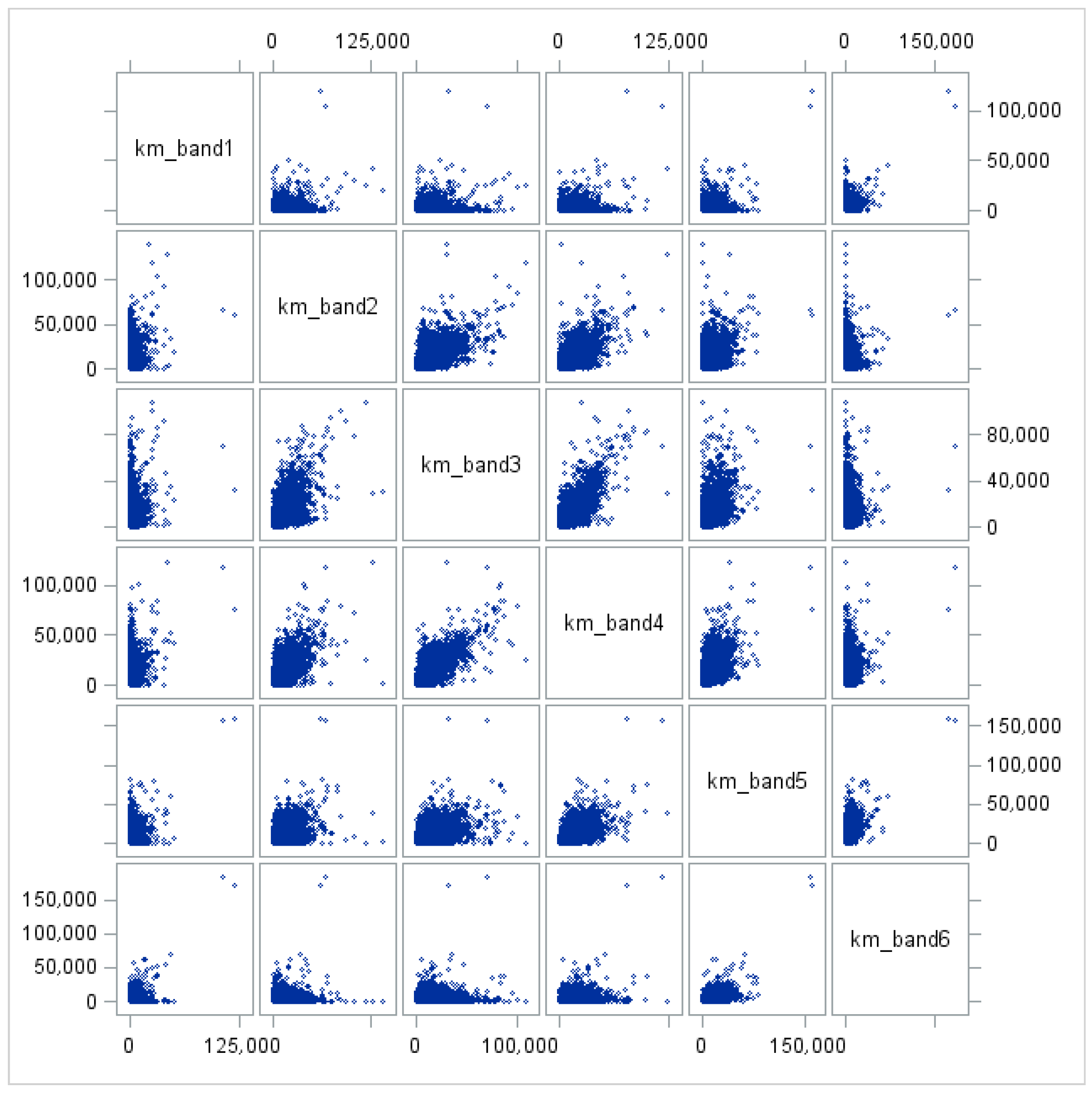
One element that emerged from the initial exploratory analyses is the strong correlation among the variables considered, as can be observed from the graphs reported below in Figure 1, Figure 2 and Figure 3.

Figure 1: Km_urb, Km_ext and Km_hig denote the number of kilometers traveled on urban roads, extra-urban roads, and highways, respectively; n_over_urb, n_over_ext and n_over_hig denote the number of speed limit violations recorded on urban roads, extra-urban roads, and highways, respectively; and Km_over_urb, Km_over_ext and Km_over_hig denote the number of kilometers driven above the speed limits on urban roads, extra-urban roads, and highways, respectively.

Figure 2: Km_band1, Km_band2, Km_band3, Km_band4, Km_band5 and Km_band6 denote the number of kilometers traveled in the following time bands, respectively: 2–5, 6–9, 10–13, 14–17, 18–21, and 22–01.

Figure 3: Tot_SA_urb, Tot_SB_urb and Tot_SC_urb represent, respectively, the number of mild accelerations, the number of mild brakings, and the number of mild turns recorded on urban roads; Tot_HA_urb, Tot_HB_urb and Tot_HC_urb represent, respectively, the number of harsh accelerations, the number of harsh brakings, and the number of harsh turns recorded on urban roads.

Correlation structures (Figure 4) very similar to those reported previously in Figure 2 also emerge from the analysis carried out on the events recorded on extra-urban roads and highways, although their graphical representation is omitted her.

Figure 4: Km_MON, Km_TUE, Km_WED, Km_THU, Km_FRI, Km_SAT and Km_SUN represent, respectively, the number of kilometers traveled by the policyholders on Monday, Tuesday, Wednesday, Thursday, Friday, Saturday, and Sunday.

It should be noted that the correlations observed in the previous graphs must be regarded as spurious, since they are dependent on a third common variable. The third variable influencing all the others can be identified as the total kilometers traveled by the policyholder/vehicle. In fact, as one would logically expect, as the number of kilometers traveled annually by the policyholder increases, the exposure to risk also increases, and consequently all the values of those variables expressed in kilometers traveled or in the number of related recorded events (for example, the number of brakings performed in a year) also increase.

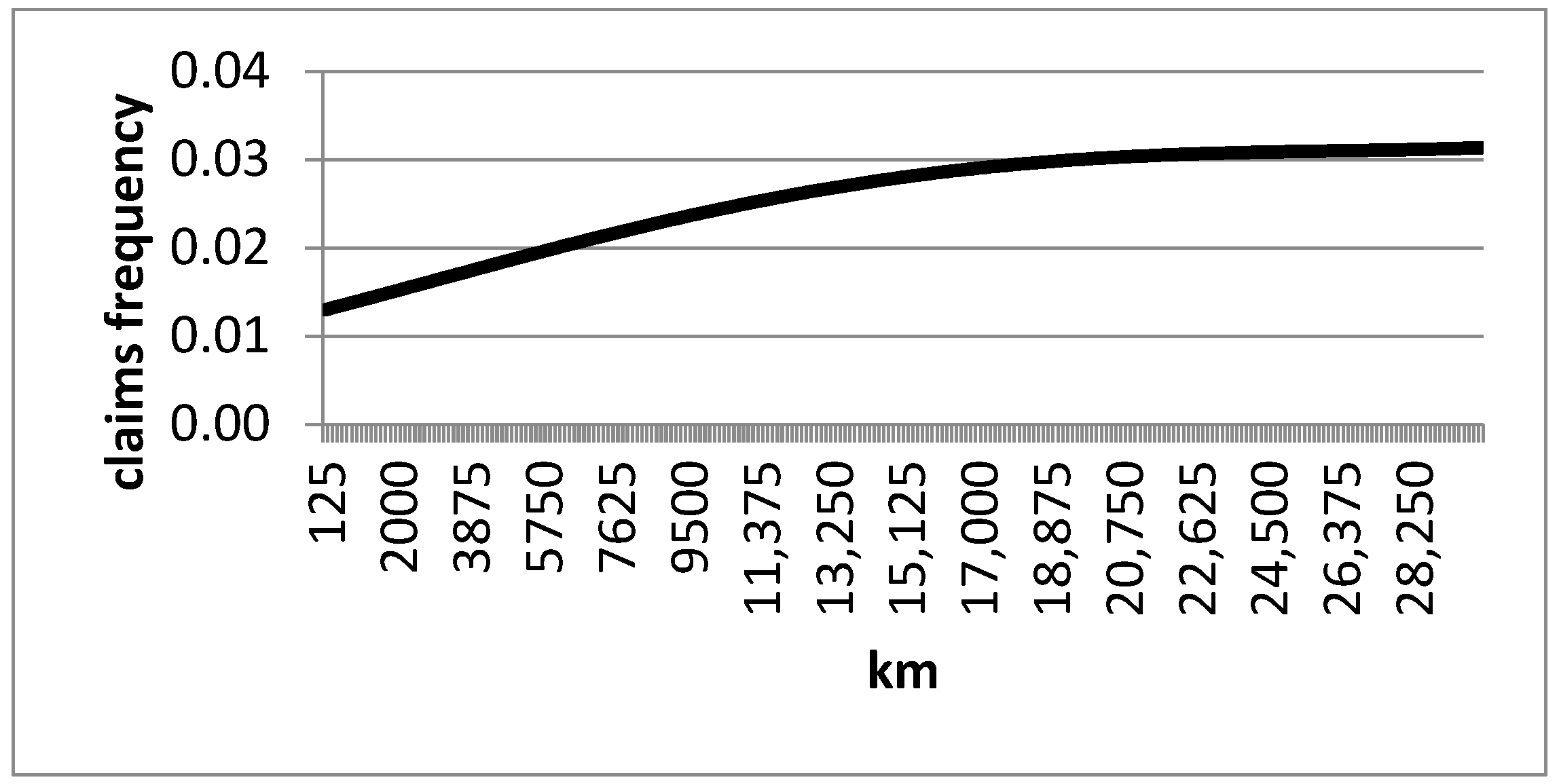
Below (Figure 5), we report the graph representing the crash frequency recorded for the different classes of annual kilometers traveled. It should be noted that the annual claim frequency increases as the annual number of kilometers traveled increases, but in a less than proportional way. This phenomenon might suggest that driving experience, and thus traveling many kilometers per year, has a relatively positive effect on claims frequency. In reality, as will be shown in the multivariate analyses, this phenomenon could be due to the kilometers traveled on highways, since those who drive many kilometers per year typically do so on highways.

In addition to this type of correlation, correlations were also found among similar variables related to the policyholder’s driving behavior: for example, those who brake frequently exhibit high values both for the variable “mild brakings” and for “harsh brakings,” and the same applies to accelerations and turns. The correlation among brakings, accelerations, and turns across different road types, however, is less evident.

These aspects have been duly taken into account in the multivariate analyses, applying transformations of the variables in order to avoid multicollinearity problems.

In order to pursue the primary objective of the rating phase, namely to determine a premium (in particular the fair premium) as closely as possible aligned with the specific claims experience of each assumed risk, univariate analyses of the variables were first carried out. These analyses made it possible to investigate the significance of the variables with respect to the claims experience of the risks under consideration.

Moreover, the variables were studied by considering separately, as response variables, the claims frequency and the average cost per claim.

Below are reported some of the variables examined for each model adopted:

• Model on claims frequency;
• Model on average costs.

5.2.1. Claims Frequency

For each variable, the claims frequencies were determined (considering as risk exposure the vehicles/years), the claims frequencies per 100,000 km traveled, and the claims frequencies per 100 h of driving.

The latter indicator was subsequently disregarded, as it does not provide additional information compared to the frequency per kilometer, being strongly correlated with it.

The following three tables (

Table 1. Age Classes—Claims Frequency.

Age	No. of Claims	No. of Policyholders	Policy/Years	Claims Frequency
G	197.00	7320.00	8792.46	2.24%
Under 21	26.00	594.00	457.76	5.68%
Under 24	166.00	2738.00	3807.02	4.36%
Under 30	379.00	8952.00	11,563.24	3.28%
Under 35	272.00	9613.00	12,254.86	2.22%
Under 45	600.00	23,451.00	26,503.91	2.26%
Under 55	610.00	23,976.00	26,018.34	2.34%
Under 60	234.00	9941.00	11,148.27	2.10%
Under 70	273.00	14,061.00	15,253.55	1.79%
Over 70	133.00	7068.00	7197.61	1.85%
Overall Total	2890.00	107,714.00	122,997.02	2.35%

,

Table 2. Age Classes—Claims Frequency per 100,000 km traveled.

Age	No. of Claims	No. of Policyholders	Km Traveled	Claims Frequency
G	197.00	7320.00	1568.39	12.56%
Under 21	26.00	594.00	49.03	53.03%
Under 24	166.00	2738.00	432.26	38.40%
Under 30	379.00	8952.00	1447.30	26.19%
Under 35	272.00	9613.00	1500.73	18.12%
Under 45	600.00	23,451.00	3051.04	19.67%
Under 55	610.00	23,976.00	3021.25	20.19%
Under 60	234.00	9941.00	1243.11	18.82%
Under 70	273.00	14,061.00	1484.60	18.39%
Over 70	133.00	7068.00	526.96	25.24%
Overall Total	2890.00	107,714.00	14,324.69	20.17%

and

Table 3. Age Classes—Claims per 100 driving hours.

Age	No. of Claims	No. of Policyholders	Driving Hours	Claims Frequency
G	197.00	7320.00	40,619.05	0.48%
Under 21	26.00	594.00	1581.10	1.64%
Under 24	166.00	2738.00	13,085.36	1.27%
Under 30	379.00	8952.00	41,480.39	0.91%
Under 35	272.00	9613.00	41,944.94	0.65%
Under 45	600.00	23,451.00	90,242.84	0.66%
Under 55	610.00	23,976.00	91,834.93	0.66%
Under 60	234.00	9941.00	37,716.49	0.62%
Under 70	273.00	14,061.00	46,961.98	0.58%
Over 70	133.00	7068.00	17,845.43	0.75%
Overall Total	2890.00	107,714.00	423,312.50	0.68%

) highlight a higher claims frequency for young drivers. Moreover, while the claims frequency determined using vehicle-years shows a sharp decrease for age classes above 30 years, this trend is less pronounced when considering the values reported per kilometers traveled and per hours of driving.

Finally, the data related to company cars present contrasting results when comparing the claims frequency calculated in the traditional way with those calculated on the basis of kilometers and hours of driving. In fact, the claims frequency of class G is in line with the average claims frequency of the portfolio, whereas the other two frequencies are well below the average.

One could conclude that the higher riskiness of company cars depends exclusively on their greater usage and, from the perspective of a per-kilometer tariff, this category should pay a lower premium than the portfolio average, disregarding for the moment the average cost per claim.

Below, we report the distribution of claims recorded in our sample, as well as the claims frequencies for each road type.

From

Table 4. Claims Distribution by Road Type.

Road Type	No. of Claims	% Claims Distribution	Km Traveled	Claims Frequency km	Driving Hours	Claims Frequency h
Urban	579	59.08%	177,931,864	32.54%	7783,735	0.74%
Extra-urban	373	38.06%	235,382,613	15.85%	5465,227	0.68%
Highway	28	2.86%	109,482,426	2.56%	1301,792	0.22%
Overall Total	980	100.00%	522,796,903	18.75%	14,550,753	0.67%

, it can be observed that the claims frequency on urban roads is higher than on other road types, since more driving hours are spent on this type of road. It should be noted that the claims frequency per kilometer on highways is very low, but it tends to increase compared to other road types when exposure is measured in driving hours. This trend is easily explained by the fact that on highways more kilometers are traveled in less time.

In this case, a low claims frequency is observed for the classes of policyholders who drive few kilometers per year. However, these policyholders prove to be very risky when the kilometers traveled are taken into account, showing claims frequencies per kilometer much higher than the portfolio average (

Table 5. Urban Roads: Annual Kilometers Traveled Class.

Annual Km Traveled	No. of Policyholders	No. of Claims	Policy/Years	Km Traveled	Claims Frequency	Claims Frequency Km
0–400	17,559	175	13,603.35	58.89	1.29%	297.15%
400–2500	22,162	459	28,429.70	1980.34	1.61%	23.18%
2500–5000	32,324	1002	42,704.36	5023.62	2.35%	19.95%
5000–10,000	29,325	1029	32,576.59	5679.69	3.16%	18.12%
>10,000	6344	225	5683.02	1582.14	3.96%	14.22%
Overall Total	107,714	2890	122,997.02	14,324.69	2.35%	20.17%

).

The same considerations made for urban roads also apply to extra-urban roads and highways, as reported in the following two tables (

Table 6. Extra-Urban Roads: Annual Kilometers Traveled Class.

Annual Km Traveled	No. of Policyholders	No. of Claims	Policy/Years	Km Traveled	Claims Frequency	Claims Frequency Km
0–400	20,980.00	264.00	16,724.35	185.43	1.58%	142.37%
400–2500	20,745.00	533.00	24,197.12	1589.24	2.20%	33.54%
2500–5000	28,037.00	806.00	35,845.14	3782.47	2.25%	21.31%
5000–10,000	23,276.00	778.00	29,732.94	4526.09	2.62%	17.19%
>10,000	14,676.00	509.00	16,497.47	4241.47	3.09%	12.00%
Overall Total	107,714.00	2890.00	122,997.02	14,324.69	2.35%	20.17%

and

Table 7. Highway: Annual Kilometers Traveled Class.

Annual Km traveled	No. of Policyholders	No. of Claims	Policy/Years	Km Traveled	Claims Frequency	Claims Frequency Km
0–200	38,297.00	696.00	35,424.48	1945.49	1.96%	35.78%
200–1000	19,299.00	646.00	25,305.66	2429.08	2.55%	26.59%
1000–4000	29,938.00	935.00	38,867.58	4898.03	2.41%	19.09%
4000–8000	12,307.00	395.00	14,933.80	2581.28	2.65%	15.30%
>8000	7873.00	218.00	8465.49	2470.80	2.58%	8.82%
Overall Total	107,714.00	2890.00	122,997.02	14,324.69	2.35%	20.17%

).

With regard to the analysis of the days of the week, after an initial examination of the individual days and based on the indications provided by the corresponding correlations, it was considered appropriate to group them into only two classes: “weekdays” (Monday to Friday) and “weekends” (Saturday and Sunday).

Below, the claims frequencies calculated for each class of annual kilometers traveled are reported separately for weekdays (

Table 8. Weekdays: Annual Kilometers Traveled Class.

Annual Km Traveled	No. of Policyholders	No. of Claims	Policy/Years	Km Traveled	Claims Frequency	Claims Frequency Km
0–500	16,676.00	161.00	12,504.09	25.30	1.29%	636.40%
500–3500	15,130.00	261.00	16,770.65	598.47	1.56%	43.61%
3500–8000	31,559.00	913.00	40,883.51	3489.77	2.23%	26.16%
8000–13000	24,194.00	847.00	30,519.77	4392.94	2.78%	19.28%
>13,000	20,155.00	708.00	22,318.99	5818.21	3.17%	12.17%
Overall Total	107,714.00	2890.00	122,997.02	14,324.69	2.35%	20.17%

) and weekends (

Table 9. Weekends: Annual Kilometers Traveled Class.

Annual Km Traveled	No. of Policyholders	No. of Claims	Policy/Years	Km Traveled	Claims Frequency	Claims Frequency Km
0–500	21,830.00	264.00	17,705.85	259.24	1.49%	101.84%
500–2000	21,941.00	518.00	27,035.48	1831.22	1.92%	28.29%
2000–4000	29,052.00	956.00	37,975.85	4289.31	2.52%	22.29%
4000–6000	19,262.00	663.00	24,152.17	3934.46	2.75%	16.85%
>6000	15,629.00	489.00	16,127.67	4010.46	3.03%	12.19%
Overall Total	107,714.00	2890.00	122,997.02	14,324.69	2.35%	20.17%

).

Also in this case, after an initial analysis of the individual time bands and based on the indications provided by the corresponding correlations, they were grouped into three classes: “day” (from 06:00 to 13:59), “evening” (from 14:00 to 21:59), and “night” (from 22:00 to 05:59).

Below, the claims frequencies calculated for each class of annual kilometers traveled are reported separately for the three variables “day” (

Table 10. Day: Annual Kilometers Traveled Class.

Annual Km Traveled	No. of Policyholders	No. of Claims	Policy/Years	Km Traveled	Claims Frequency	Claims Frequency Km
0–400	17,666.00	194.00	13,368.49	38.34	1.45%	505.94%
400–2500	20,036.00	491.00	23,736.24	1199.69	2.07%	40.93%
2500–5000	29,837.00	941.00	39,220.53	3879.05	2.40%	24.26%
5000–10,000	29,336.00	931.00	35,018.03	5669.20	2.66%	16.42%
>10,000	10,839.00	333.00	11,653.74	3538.40	2.86%	9.41%
Overall Total	107,714.00	2890.00	122,997.02	14,324.69	2.35%	20.17%

), “evening” (

Table 11. Evening: Annual Kilometers Traveled Class.

Annual Km Traveled	No. of Policyholders	No. of Claims	Policy/Years	Km Traveled	Claims Frequency	Claims Frequency Km
0–400	17,422.00	176.00	13,149.92	37.32	1.34%	471.58%
400–3000	20,161.00	409.00	23,450.49	1065.42	1.74%	38.39%
3000–6000	29,563.00	889.00	38,817.04	3700.37	2.29%	24.02%
6000–10,000	25,426.00	920.00	31,476.86	4954.44	2.92%	18.57%
>10,000	15,142.00	496.00	16,102.71	4567.13	3.08%	10.86%
Overall Total	107,714.00	2890.00	122,997.02	14,324.69	2.35%	20.17%

), and “night” (

Table 12. Night: Annual Kilometers Traveled Class.

Annual Km Traveled	No. of Policyholders	No. of Claims	Policy/Years	Km Traveled	Claims Frequency	Claims Frequency Km
0–100	29,034.00	351.00	24,731.91	818.66	1.42%	42.88%
100–500	24,254.00	574.00	29,522.91	2712.10	1.94%	21.16%
500–1500	28,088.00	848.00	36,563.46	4764.92	2.32%	17.80%
1500–3000	15,624.00	620.00	19,907.20	3228.69	3.11%	19.20%
>3000	10,714.00	497.00	12,271.54	2800.33	4.05%	17.75%
Overall Total	107,714.00	2890.00	122,997.02	14,324.69	2.35%	20.17%

).

In general, exceeding the legally imposed speed limits is considered to be among the main causes of road accidents. In the following two tables (

Table 13. Annual Km Traveled above the Speed Limit.

Annual Km Over Limit	No. of Policyholders	No. of Claims	Policy/Years	Km Traveled	Claims Frequency	Claims Frequency Km
0–300	27,156.00	376.00	23,667.86	560.87	1.59%	67.04%
300–1000	24,248.00	620.00	29,234.59	2203.52	2.12%	28.14%
1000–3000	32,996.00	1125.00	42,394.93	5355.96	2.65%	21.00%
>3000	23,314.00	769.00	27,699.63	6204.33	2.78%	12.39%
Overall Total	107,714.00	2,890.00	122,997.02	14,324.69	2.35%	20.17%

and

Table 14. Annual Number of Speed Limit Violations.

Annual No. Over Limit	No. of Policyholders	No. of Claims	Policy/years	Km traveled	Claims Frequency	Claims Frequency Km
0–150	26,727.00	361.00	22,672.23	438.46	1.59%	82.33%
150–700	27,781.00	730.00	34,017.86	2700.33	2.15%	27.03%
700–2000	30,801.00	1047.00	39,993.20	5225.11	2.62%	20.04%
>2000	22,405.00	752.00	26,313.74	5960.79	2.86%	12.62%
Overall Total	107,714.00	2890.00	122,997.02	14,324.69	2.35%	20.17%

), the claims frequencies are reported, calculated on the basis of the annual kilometers traveled above the limits and on the number of speed limit violations recorded in a year.

Both variables show a claims frequency that increases with the number of kilometers traveled above the speed limit and with the number of speed limit violations, whereas the claims frequency per kilometer decreases as the annual kilometers and the annual number of speed limit violations increase. This latter result is strongly influenced by the fact that policyholders who drive more kilometers in a year exhibit a lower claims frequency per kilometer. This phenomenon may depend on the greater driving experience of the policyholder or on the fact that many of these kilometers are traveled on highways.

Below (

Table 15. Km Traveled in a Year: Annual Km Traveled Class.

Annual Km Traveled	No. of PolicyHolders	No. of Claims	Policy/Years	Km Traveled	Claims Frequency	Claims Frequency Km
0–250	11,369.00	96.00	8465.14	6.48	1.13%	1481.68%
250–4000	15,384.00	246.00	14,989.32	305.78	1.64%	80.45%
4000–7000	13,745.00	344.00	17,734.27	1011.89	1.94%	34.00%
7000–9000	10,147.00	289.00	13,590.56	1112.43	2.13%	25.98%
9000–12,000	14,931.00	483.00	19,680.04	2104.03	2.45%	22.96%
12,000–15,000	12,260.00	424.00	15,629.40	2137.48	2.71%	19.84%
15,000–20,000	13,819.00	481.00	16,157.11	2825.34	2.98%	17.02%
>20,000	16,059.00	527.00	16,751.20	4821.27	3.15%	10.93%
Overall Total	107,714.00	2890.00	122,997.02	14,324.69	2.35%	20.17%

), the claims frequencies calculated for different classes of annual kilometers traveled are reported.

For each of the other factors aimed at capturing the policyholder’s driving style (accelerations, brakings, and turns), two variables were created based on the severity of the recorded event. Accordingly, the variables analyzed are: mild and harsh accelerations (

Table 16. Harsh accelerations (HA).

Annual No. of HA	No. of Policyholders	No. of Claims	Policy/Years	Km Traveled	Claims Frequency	Claims Frequency Km
0	2726.00	56.00	908.67	37.89	6.16%	147.81%
>0	217.00	6.00	72.33	5.57	8.29%	107.62%
Overall Total	2943.00	62.00	981.00	43.46	6.32%	142.65%

), mild and harsh brakings (

Table 17. Harsh brakings (HB).

Annual No. of HB	No. of Policyholders	No. of Claims	Policy/Years	Km Traveled	Claims Frequency	Claims Frequency Km
0	909.00	10.00	303.00	3.25	3.30%	307.56%
0–50	1346.00	27.00	448.67	22.72	6.02%	118.82%
>50	688.00	25.00	229.33	17.49	10.90%	142.97%
Overall Total	2943.00	62.00	981.00	43.46	6.32%	142.65%

), mild and harsh turns (

Table 18. Harsh turns (HT).

Annual No. of HT	No. of Policyholders	No. of Claims	Policy/Years	Km Traveled	Claims Frequency	Claims Frequency Km
0	855.00	8.00	285.00	2.19	2.81%	365.58%
0–30	893.00	22.00	297.67	13.28	7.39%	165.70%
>30	1195.00	32.00	398.33	28.00	8.03%	114.30%
Overall Total	2943.00	62.00	981.00	43.46	6.32%	142.65%

).

Below, the univariate analyses carried out on these variables defined as “harsh” are reported.

For these latter variables as well, a dependency on the number of kilometers traveled can be observed. In particular, for most variables it is noted that the claims frequency increases with the number of recorded DB events, but once the frequency is adjusted for the effect of kilometers traveled, the relationship between claims frequency and the number of DB events is reversed.

For each individual variable previously examined, the Wald test was performed in order to verify their statistical significance. Specifically, each variable was related to the response variables (claims frequency and claims frequency per kilometer) within a univariate model. Below (

Table 19. Wald Test for Univariate Analyses.

Variables	p-Value (Policy/Years)	p-Value (Km)
Age Class	<0.0001	<0.0001
Territorial Area	<0.0001	<0.0001
Vehicle Registration Year	0.0272	<0.0001
Urban Km Class	<0.0001	<0.0001
Extra-Urban Km Class	<0.0001	<0.0001
Highway Km Class	<0.0001	<0.0001
Weekday Km Class	<0.0001	<0.0001
Weekend Km Class	<0.0001	<0.0001
Daytime Km Class	<0.0001	<0.0001
Evening Km Class	<0.0001	<0.0001
Night Km Class	<0.0001	<0.0001
Mild Acceleration Class	0.0006	0.0701
Mild Braking Class	0.0968	0.7172
Mild Turning Acceleration Class	0.2028	0.0065
Harsh Acceleration Class	0.5531	0.5427
Harsh Braking Class	0.0106	0.3641
Harsh Turning Acceleration Class	0.0736	0.2082
Kilometers Traveled Over Limit	<0.0001	<0.0001
Number of Over Limit	<0.0001	<0.0001
Annual Kilometers Class	<0.0001	<0.0001

), the p-values resulting from the tests are reported.

All the variables considered individually, with the exception of some DB variables, turn out to be significant. It should be emphasized once again that this result is strongly influenced by the spurious correlation existing among the variables. With regard to DB variables, the only significant one is “harsh brakings”.

5.2.2. Average Claim Cost

Starting from the sample data on claim costs, the total cost borne by the company for each claim was calculated. In the analysis of average costs, the direct compensation system was taken into account.

For all the variables studied, the Kruskal–Wallis test was performed in order to verify their statistical significance. The Kruskal–Wallis test, also known as the nonparametric analysis of variance for a single classification factor, can be regarded as an extension of the Wilcoxon–Mann–Whitney test, based on ranks.

Below (

Table 20. Kruskal–Wallis Test.

Variables	p-Value
Age Class (Figure 7)	0.0185
Territorial Area	0.1836
Vehicle Registration Year	0.1359
Urban Km Class	0.0093
Extra-Urban Km Class	0.3855
Highway Km Class	0.842
Weekday Km Class	0.096
Weekend Km Class	0.0318
Daytime Km Class	0.386
Evening Km Class	0.55
Night Km Class	0.1126
Kilometers Traveled Over Limit	0.1128
Number of Over Limit	0.0261
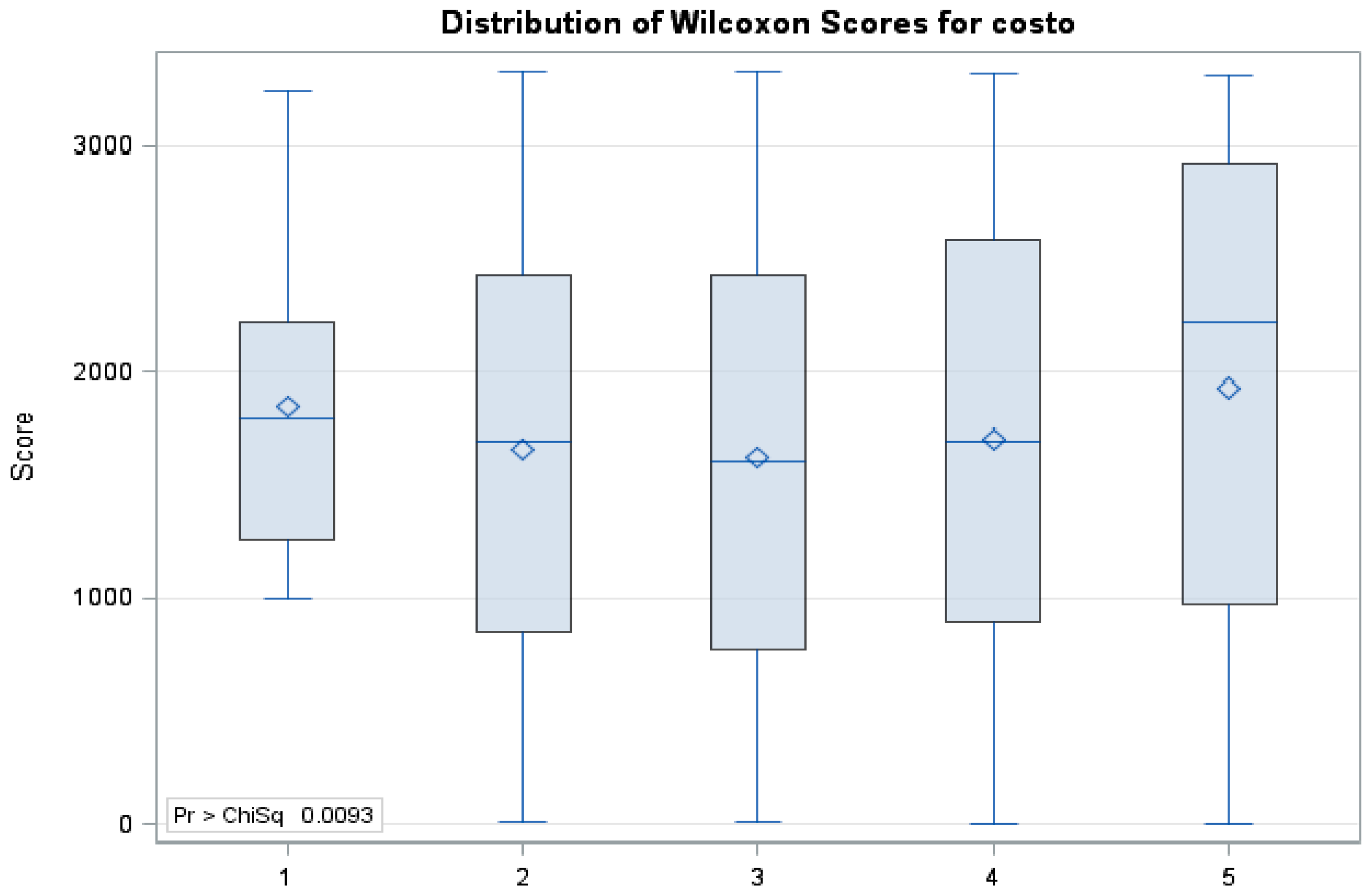
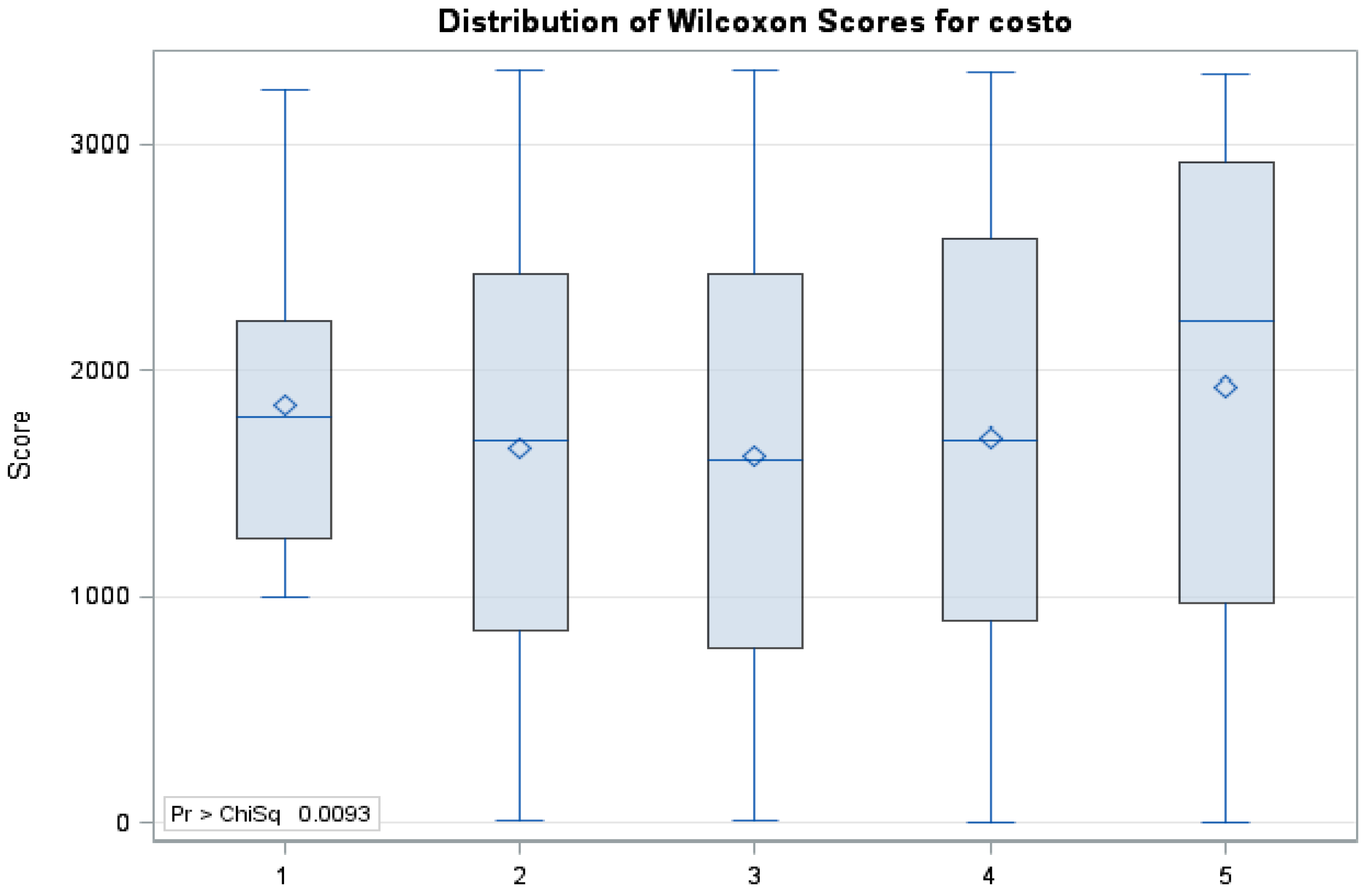
Annual Kilometers Class	0.1018

), the results of the Kruskal–Wallis test performed on each individual variable are reported. In addition, for the variables found to be significant, the corresponding box plots (Figure 6, Figure 7, Figure 8, Figure 9) are provided.

Classes 1–5 (Figure 6) shown in the previous chart are decoded as follows: 0–400; 400–2500; 2500–5000; 5000–10,000, and greater than 10,000.

Figure 7. Box Plot—Age Class.

Figure 7. Box Plot—Age Class.

Classes 1–4 (Figure 8) shown in the following chart are decoded as follows: 0–150; 150–700; 700–2000, greater than 2000.

Figure 8. Box Plot—No. Over Limit.

Figure 8. Box Plot—No. Over Limit.

Classes 1–5 (Figure 9) shown in the following chart are decoded as follows: 0–500; 500–2000; 2000–4000; 4000–6000, and greater than 6000.

Figure 9. Box Plot—Kilometers Traveled on Weekends.

Figure 9. Box Plot—Kilometers Traveled on Weekends.

5.3. Tariff Modeling Analysis

Two separate statistical models were constructed for claims frequency and for average claim cost. The models employed fall within the framework of Generalized Linear Models (GLMs) and, depending on the scope of the analysis, provide nonlinear regressions for the two phenomena.

In particular, for claims frequency three different distributions were examined:

Poisson Model:

GLM with logarithmic link function and Poisson probability structure:

$$\mathrm{Pr}\left(Y=y\right)={\displaystyle \frac{e^{-\lambda }{\lambda }^y}{y!}}$$

Negative Binomial Model:

GLM with logarithmic link function and Negative Binomial probability structure:

$$Pr\left(Y=y\right)=\left(\begin{array}{c}y-1\\ k-1\end{array}\right)p^k{\left(1-p\right)}^{y-k}\hspace{1em}\hspace{1em}\forall y=k, k+1, \dots$$

Zero-Inflated Poisson Model:

GLM with logarithmic link function and probability structure given by the mixture of a degenerate distribution at zero and a Poisson distribution:

$$Pr\left(Y=y\right)=\left\{\begin{array}{c}\varphi +\left(1-\varphi \right)e^{-\lambda }\hspace{1em}\hspace{1em}\hspace{1em}y=0\\ \left(1-\varphi \right){\displaystyle \frac{e^{-\lambda }{\lambda }^y}{y!}}\hspace{1em}\hspace{1em}\hspace{1em}y\ne 0\end{array}\right.$$

Moreover, in order to account not only for exposure expressed in vehicles/year but also for that expressed in kilometers traveled, the following offset variables were introduced for each GLM: vehicles/year and kilometers traveled (divided by 100,000).

All baseline models were constructed considering the following variables:

• Age class;
• Vehicle registration Year;
• Total kilometers traveled in a year by each policyholder;
• Geographical area, constructed through a cluster analysis on the provinces included in the dataset;
• Number of times the speed limit is exceeded per 1000 km on the three different types of roads (urban, extra-urban, highway);
• Percentages of kilometers traveled on the three different types of roads relative to total kilometers traveled;
• Percentages of kilometers traveled above the speed limit relative to total kilometers traveled on the three different types of roads;
• Percentages of kilometers traveled on weekdays relative to the total kilometers traveled during the week;
• Percentages of kilometers traveled on weekends relative to the total kilometers traveled during the week;
• Percentages of kilometers traveled during daytime relative to the total kilometers traveled over 24 h;
• Percentages of kilometers traveled during evening relative to the total kilometers traveled over 24 h;
• Percentages of kilometers traveled during nighttime relative to the total kilometers traveled over 24 h.

The selection procedure used to determine a subset of significant explanatory variables was the backward method. Therefore, from the adopted model, variables whose inclusion did not increase, or even decreased, explanatory power to explain the variability of the phenomenon were eliminated.

Below (

Table 21. Poisson Model—Exposure in Vehicles/Year—Final Set of Variables.

Variables	p-Value
Age Class	<0.0001
Annual Kilometers Class	<0.0001
Territorial Area	<0.0001
% of Kilometers Traveled on Urban Roads	<0.0001
% of Kilometers Traveled on Highways	0.0125
% of Kilometers Traveled Above the Speed Limit on Urban Roads	0.0357
% of Kilometers Traveled on Weekdays	<0.0001
% of Kilometers Traveled During Daytime	<0.0001
% of Kilometers Traveled During Night	0.0001

and

Table 22. Negative Binomial Model—Exposure in Vehicles/Year—Final Set of Variables.

Variables	p-Value
Age Class	<0.0001
Annual Kilometers Class	<0.0001
Territorial Area	<0.0001
% of Kilometers Traveled on Urban Roads	<0.0001
% of Kilometers Traveled on Highways	0.013
% of Kilometers Traveled Above the Speed Limit on Urban Roads	0.0417
% of Kilometers Traveled on Weekdays	<0.0001
% of Kilometers Traveled During Daytime	<0.0001
% of Kilometers Traveled During Nighttime	0.0002

), the Wald tests performed for all models constructed with the final variables are presented.

With regard to the models based on the Poisson and the Negative Binomial distributions, it should be noted that the final models are very similar to each other, both in terms of the variables selected and the p-values obtained for each variable. In both cases, among the most significant variables, as expected, are the total annual kilometers, age, and geographical area.

The model based on the ZIP distribution also highlights the same variables found to be significant in the other two models. It should be noted, in the tables reported below (

Table 23. ZIP Model—Exposure in Vehicles/Year—Final Set of Variables.

Variables	p-Value
Age Class	<0.0001
Territorial Area	<0.0001
% of Kilometers Traveled on Urban Roads	<0.0001
% of Kilometers Traveled Above the Speed Limit on Urban Roads	0.0147
% of Kilometers Traveled Above the Speed Limit on Extra-Urban Roads	<0.0001
% of Kilometers Traveled Above the Speed Limit on Highway	0.0153
Number of Over-Limit Events on Urban Roads	0.0026
% of Kilometers Traveled on Weekdays	<0.0001
% of Kilometers Traveled During Nighttime	<0.0001
Variables—Zero Inflation Model	p-Value
Annual Kilometers Class	<0.0001
% of Kilometers Traveled Above the Speed Limit on Extra-Urban Roads	<0.0001
Number of Over-Limit Events on Urban Roads	<0.0001
Number of Over-Limit Events on Highway	<0.0001
% of Kilometers Traveled on Weekdays	0.0125
% of Kilometers Traveled During Evening	<0.0001
% of Kilometers Traveled During Nighttime	0.0001

and

Table 24. Comparison of Models for Claims Frequency per Vehicles/Year.

Measures	Poisson	Negative Binomial	ZIP
Deviance	18,734.15	16,991.92	24,182.09
Log-Likelihood	−12,040.26	−12,014.76	−11,976.03
AIC	24,394.55	24,345.54	24,316.09
Scaled Pearson	127,111.29	124,889.73	122,283.24

), that the variable “total annual kilometers” is significant only for the “zero-inflation” component, i.e., for explaining the probability of having zero claims, whereas the “geographical area” is significant only for the Poisson component.

Above (Table 24) are reported the goodness-of-fit measures calculated for the purpose of comparing the models. Based on the results of the calculated measures, it can be concluded that the model based on the ZIP distribution is better able to explain the variability of the phenomenon, presenting a lower value of both the AIC and the Scaled Pearson statistic, and a higher value of the log-likelihood.

In the following tables (

Table 25. Poisson Model—Exposure in kilometers—Final Set of Variables.

Variables	p-Value
Age Class	<0.0001
Annual Kilometers Class	<0.0001
Territorial Area	<0.0001
% of Kilometers Traveled on Urban Roads	<0.0001
% of Kilometers Traveled on Highways	0.0002
% of Kilometers Traveled on Weekends	<0.0001
% of Kilometers Traveled During Daytime	<0.0001
% of Kilometers Traveled During Night	0.001

and

Table 26. Negative Binomial Model—Exposure in kilometers—Final Set of Variables.

Variables	p-Value
Age Class	<0.0001
Annual Kilometers Class	<0.0001
Territorial Area	<0.0001
% of Kilometers Traveled on Urban Roads	<0.0001
% of Kilometers Traveled on Highways	0.0002
% of Kilometers Traveled on Weekends	<0.0001
% of Kilometers Traveled During Daytime	<0.0001
% of Kilometers Traveled During Night	0.001
Age Class	<0.0001

), the tests are reported using kilometers traveled as the exposure, in order to identify the set of significant variables for claims frequency per kilometer.

As was highlighted for the models with exposure in vehicles/year, these latter two models (Poisson and Negative Binomial) also present the same variables in the final model, with very similar p-values.

In this latter model (

Table 27. ZIP Model—Exposure in kilometers—Final Set of Variables.

Variables	p-Value
Age Class	<0.0001
% of Kilometers Traveled on Urban Roads	<0.0001
% of Kilometers Traveled Above the Speed Limit on Urban Roads	0.0029
% of Kilometers Traveled Above the Speed Limit on Extra-Urban Roads	<0.0001
% of Kilometers Traveled on Weekdays	<0.0001
% of Kilometers Traveled During Night	<0.0001
Variables—Zero Inflation Model	p-Value
% of Kilometers Traveled on Urban Roads	<0.0001
% of Kilometers Traveled Above the Speed Limit on Urban Roads	<0.0001
% of Kilometers Traveled Above the Speed Limit on Extra-Urban Roads	<0.0001
% of Kilometers Traveled on Weekdays	<0.0001
% of Kilometers Traveled During Nighttime	00.0491

), for the zero-inflation component, variables widely used in personalization techniques adopted by insurance companies—age and geographical area—did not result as significant. Age is significant only for the Poisson component.

It should be emphasized, however, that this model is less capable of explaining portfolio variability compared to the Poisson and Negative Binomial models, as can be seen from the following tables (

Table 28. Comparison of Models for Claims Frequency per Kilometer.

Measures	Poisson	Negative Binomial	ZIP
Deviance	19,231.55	19,231.55	25,264.48
Log-Likelihood	−12,288.96	−12,288.96	−12,517.23
AIC	24,881.96	24,883.96	25,370.48
Scaled Pearson	252,014.01	252,014.03	417,747.32

).

Below (

Table 29. Average claim cost—Final Set of Variables.

Variables	p-Value
% of Kilometers Traveled on Urban Roads	0.031
% of Kilometers Traveled on Extra-Urban Roads	0.0215

) is reported the Wald test performed for the model on average claim costs.

Given that the sum of the percentages of kilometers traveled on urban roads, extra-urban roads, and highways equals 1, one of the three was removed from the model in order to avoid multicollinearity issues. Therefore, it can be concluded that the only significant information is that related to mileage on the different types of roads.

6. Conclusions and Insights

Numerous insights and reflections emerge from the analyses carried out, as well as from further future analyses that may be conducted on telematics data.

Among the main advantages of the use and dissemination of black boxes, we can certainly highlight the opportunity to broaden the range of products offered to policyholders, thereby improving market competition. As shown by the study, black box data find their most effective application in the design phase of the pricing scheme. Not only is it possible to discriminate risks more accurately at portfolio entry, but it also becomes possible to construct a clear and transparent pricing scheme in which costs depend on the actual risk exposure of the policyholder and, therefore, on how, when, and how much the policyholder drives.

For example, using the information extracted from the black box and the results obtained from the analysis, it was possible to construct merit/demerit indices based not only on the number of claims that occurred, but also on policyholder behaviors that affect the probability of a claim occurring.

Below is reported one possible example of the merit/demerit index, obtained by selecting only two variables for simplicity: the number of kilometers driven at night and the total annual kilometers driven. Clearly, this represents just one of the many possible solutions that can be derived from the analysis.

From

Table 30. Merit/Demerit Index.

Merit Class	Merit/Demerit Indices	Km Traveled Night			Annual Km Traveled
		0–20%	20–60%	>60%	0–5000	5000–10,000	>10,000
1	0.27	X			X
2	0.37	X				X
3	0.43		X		X
4	0.48	X					X
5	0.55			X	X
6	0.60		X			X
7	0.77		X				X
8	0.87			X		X
9	1.00			X			X

, it can be observed, for example, that the merit index to be applied to a policyholder who drives annually between 0 and 5000 km, of which at most 20% are driven at night, is equal to 0.27.

In the same way, it is possible to construct the merit/demerit index by selecting two or more variables different from total kilometers driven and kilometers driven at night.

In general, a priori rating is performed by differentiating policyholders through traditional variables that can already be observed at the time of signing the first insurance contract. These variables generally describe the objective characteristics of the policyholder and the vehicle.

If information on mileage and/or driving behavior of policyholders were available, it would be possible to include “experience variables” already in a priori personalization, thus allowing the use of the models analyzed in the previous sections also at policy inception.

In any case, using information obtained from the black box, it is possible to construct merit/demerit indicators (bonus/malus) based not exclusively on occurred claims, but on policyholder behaviors that increase or decrease the probability of a claim occurring. Once a model is defined that distinguishes between “good” and “bad” policyholders, a new bonus/malus variable can be introduced into the set of variables used for personalized premium determination.

Moreover, in the case of a mileage-based pricing schemes, some experience variables could be incorporated into the a priori rating, defining a cost per kilometer that varies according to where and/or when the kilometer is driven (for example, by assigning a different premium for kilometers traveled at night compared to those traveled during the day).

This additional information could foster the development of innovative insurance solutions for motor liability contracts, such as the following:

• Prepaid kilometer schemes, where the policyholder knows the cost per kilometer under different driving conditions and they pay in advance for coverage of a fixed number of kilometers rather than for a time period;
• Pay-per-bill schemes, where the policyholder pays at regular intervals (e.g., every one/two months) based on the kilometers driven, taking into account how, where, and when they were driven;
• Points-based schemes, where coverage is gradually consumed depending on driving style (e.g., points are reduced for harsh accelerations, sharp turns, kilometers driven under adverse conditions, or other predefined DB events).

7. Future Benefits and Developments

The availability of richer technical data could also enable companies that do not use telematics data directly for pricing purposes not only to select a portfolio of safer policyholders, but also to gain a better understanding of their portfolio, monitoring its riskiness through black box data.

Moreover, models based on estimates derived from GLMs could be employed for determining the best estimate of unearned premium reserves, as well as the corresponding SCR and Fair Value.

Additional advantages should not be overlooked from the information that can be obtained ex post from black boxes after an accident occurs, which could both reduce fraud and provide further insights for calculating reserves. For example, one can imagine a model that, based on black box data—such as impact severity, vehicle model, accident dynamics, and point of impact—can estimate the claim amount, useful both for fraud detection and for reserving purposes.

Further advantages from the use of black boxes can be observed at the level of the entire insurance system: benefits would accrue, both directly and indirectly, to citizens in terms of greater road safety and reduced environmental impact, contributing to lower CO₂ emissions and improved driving behavior, thus reducing accident incidence and its consequences.

The improvement in claims experience within the insurance system can be attributed to two interconnected factors: fraud reduction and optimization of driving behavior. The use of black boxes allows for objective and continuous monitoring of driving dynamics, reducing opportunities for insurance fraud by providing verifiable data that either confirm or contradict policyholder statements. This leads to a decrease in claims frequency and, consequently, a reduction in average claim costs. At the same time, real-time feedback encourages drivers to modify risky behaviors, resulting in fewer accidents and an overall improvement in road safety, with positive systemic effects on insurance costs.