1. Introduction
This survey offers a concise overview of the General Framework of Portfolio Theory (GFPT). Developed in the 1950s, portfolio theories primarily followed two schools of thought. The first, championed by
Markowitz (
1959), emphasizes portfolio selection as a trade-off between reward and risk. The second focuses on seeking the optimal portfolio for maximum growth (see
Kelly 1956;
Lintner 1965;
MacLean et al. 2011). However, as portfolio theories evolved, it became evident that Markowitz’s use of variance as a risk measure was not entirely satisfactory. The single-minded pursuit of portfolio returns without adequately addressing risk posed its own set of dangers. Consequently, the analysis of risk measures gained prominence among researchers and practitioners, leading to a fruitful area of financial analysis, cf.
Artzner et al. (
1999);
Carr and Zhu (
2018). The GFPT unifies these three areas of research, and establishes a robust mathematical foundation. It is noteworthy that the concavity of the reward management function, driven by risk aversion, and the convexity of the risk measure, attributed to the risk-reducing effects of diversification, make convex analysis and duality central to this framework (see
Carr and Zhu 2018;
Maier-Paape et al. 2023).
Furthermore, practical problems, such as bank balance sheet management dealing with multiple risks of different properties, necessitate the extension of the theory to encompass the analysis of vector risks. Our goal here is to provide readers with a quick guided tour of the most important results from the General Framework of Portfolio Theory and demonstrate its practical applications. We aim to emphasize key ideas without delving into excessive technical details, refraining from providing proofs. Instead, we highlight selected proof concepts and direct interested readers to the monograph (
Maier-Paape et al. 2023) for in-depth details.
Forerunner of this monograph with respect to laying the basic ideas of the General Framework of Portfolio Theory has been the work of
Maier-Paape and Zhu (
2018a), followed by
Maier-Paape and Zhu (
2018b) and
Maier-Paape et al. (
2019), the latter two including drawdown risk and multi-period markets. Furthermore,
Platen (
2018) contributed significantly to the GFPT by his modular approach, before lastly
Maier-Paape et al. (
2023) picked up all these ideas, brought them together and crucially extended them by allowing vector risk.
To limit the length of the paper, we have chosen to focus on the main ideas and results of GFPT, necessitating the omission of several important related topics. These include portfolio theory for continuous stochastic market models (cf.
Fouque et al. 2017;
Merton 1992), as well as issues related to hedging and replicating financial derivatives. Additionally, we have not covered strategies for limiting the risk of growth-optimal portfolios over a finite time horizon, which involves analyzing nonconcave reward functions (see
Dewasurendra et al. 2019;
Lopez de Prado et al. 2019;
Vince and Zhu 2015).
In the next section, we embark on a detailed exploration of the historical underpinnings of the GFPT. We then turn our attention into the simpler case, which involves scalar risk alone.
Section 3 will elucidate the efficient frontier, while
Section 4 will examine the associated efficient portfolios. Additionally,
Section 5 will analyze the behavior of the efficient frontier at its boundaries. Moving forward to
Section 6, we will explore the broader scope of portfolio theory, incorporating vector risk. Our survey culminates in
Section 7. To aid readers, two appendices have been included, offering reviews on semi-continuity and financial markets for added clarity and convenience.
3. The Efficient Frontier within the General Framework of Portfolio Theory for Scalar Risk
In this and the following two sections, we outline the basics of the General Framework of Portfolio Theory (GFPT) for scalar risk. Our exposition is based on the recent book of
Maier-Paape et al. (
2023). Here, however, we restrict ourselves to presenting the main results and some main ideas of proofs. Central to this theory are so-called “admissible” portfolios with
components,
:
Definition 2 (Admissible portfolios;
Maier-Paape et al. 2023, Definition 2.7)
. We say that is a set of admissible portfolios
, provided that A is Notation 1 (Risky parts of portfolios;
Maier-Paape et al. 2023, Notation 2.8)
. We define the risky parts
of the admissible portfolios as The theory will always deal with portfolios from the admissible set
, where we distinguish for
the component
, which stands for a risk-free investment, and
, which stands for
M risky investments. This models a financial market consisting of a scalar risk-free bond and
M risky assets (see Definition A3 in
Appendix A).
The other two ingredients for the General Framework of Portfolio Theory are risk and utility functions, both of which are defined on the set of admissible portfolios. Hence, we continue with the abstract definition of a risk function and include some relevant properties, before we follow up with the definition of a utility function.
Assumption 1 (Risk functions;
Maier-Paape et al. 2023, Assumption 2.20)
. Consider an extended-valued risk function
on the admissible portfolios (cf. Definition 2). We always assume risk functions to be lower semi-continuous (see Definition A1 in Appendix A). Furthermore, we will often use some of the following properties:- (r1)
(Riskless asset contributes no risk) The risk function is a function of only the risky part of the portfolio, where , i.e., (cf. Notation 1).
- (r1n)
(Non-negativity and normalization) The risk function is non-negative, i.e., for all , and there is at least one portfolio of purely bonds in A. Furthermore, if and only if contains only a riskless bond, i.e., for some .
- (r2)
(Diversification reduces risk) The risk function is proper convex.
- (r2s)
(Diversification strictly reduces risk) The risk function is strictly convex on its .
Remark 1 (Usual assumptions regarding risk functions in GFPT). For a valid risk function in terms of the GFPT, it has to satisfy either (r2) or (r2s). However, the conditions (r1) and (r1n) are not necessary for the theory presented here to hold, although they are often satisfied in applications.
Assumption 2 (Utility functions;
Maier-Paape et al. 2023, Assumption 2.29)
. Consider an extended-valued utility function
on the admissible portfolios A (cf. Definition 2). We will always assume utility functions to be upper semi-continuous (see Remark A2 in Appendix A). Furthermore, we often use some of the following properties:- (u2)
(Diminishing marginal utility) The utility function is proper concave.
- (u2s)
(Strict diminishing marginal utility) The utility function is strictly concave on its domain .
Example 1 (Markowitz risk and utility)
. The probably most well-known utility function is expected return
from Markowitz,where is the risky part of the payoff of a one-period financial market (cf. Definitions A3 and A4 in Appendix A). Note that is linear in x, such that (u2)
is satisfied, but not (u2s)
. On the other hand, using Notation A1 in Appendix A, we definewhich is known as Markowitz volatility
. It satisfies (r1)
and (r2)
. However, under further assumptions on the financial market, such as the so-called “no nontrivial riskless portfolio” condition (cf. Definition A5 in Appendix A), and with from (7), even (r1n)
is satisfied, and satisfies (r2s)
on its domain (see Example A1 in Appendix A for more details). We provide further examples of utility and risk functions in Examples A2 and A3 in Appendix A, respectively. Using a set of admissible portfolios A (cf. Definition 2), as well as an extended-valued risk function and an extended-valued utility function , the following compactness assumption is essential for most of the results of the GFPT (see also Assumption 4).
Assumption 3 - (a)
;
- (b)
For all , the setsare compact in .
Points
, which may be represented as
contribute to the so-called “
risk–utility space”
defined in (
10) below. We continue with some basic properties of
.
Proposition 1 (Basic properties of
;
Maier-Paape et al. 2023, Proposition 2.58)
. Assume that is a set of admissible portfolios, as in Definition 2. Moreover, assume the risk function satisfies (r2)
in Assumption 1, and assume the utility function satisfies (u2)
in Assumption 2. We claim:- (a)
- (b)
- (c)
Assume furthermore that Assumption 3(b) holds. Then, the set is closed.
Investors generally prefer portfolios either with lower risk for a given utility value, or with higher utility for a given risk value. Thus, portfolios which cannot be “improved” are called efficient.
Definition 3 (Efficient portfolios;
Maier-Paape et al. 2023, Definition 2.59)
. We say that a portfolio with and is Pareto efficient
(for the risk function , the utility function , and admissible portfolios A), provided that there does not exist any , such that eitherorholds. Definition 4 (Efficient frontier;
Maier-Paape et al. 2023, Definition 2.60)
. We call the set of images of all efficient portfolios in the two-dimensional risk–utility space, i.e.,the efficient frontier.
Analogously as in standard portfolio theory, the efficient frontier is essential in the GFPT as well. We continue with some basic and straight forward properties of the efficient frontier , and some relations to the risk–utility space .
Theorem 1 (Efficient frontier properties;
Maier-Paape et al. 2023, Theorem 2.61)
. Assume again the situation of Proposition 1. Then, the following holds true:- (a)
Efficient portfolios represented in the two-dimensional risk–utility space all lie on the boundary of .
- (b)
cannot contain vertical or horizontal line segments (of positive length).
- (c)
In the case where furthermore Assumption 3(b) holds, then has the following representation:
The so-called “standing assumptions” below collect these assumptions on and , which are necessary for the main results on the efficient frontier to come.
Assumption 4 (Standing assumptions for
and
;
Maier-Paape et al. 2023, Assumption 2.64)
. We assume the following properties:- (a)
is a set of admissible portfolios, according to Definition 2.
- (b)
is a lower semi-continuous extended-valued risk function satisfying (r2) in Assumption 1.
- (c)
is an upper semi-continuous extended-valued utility function satisfying (u2) in Assumption 2.
- (d)
Assumption 3, concerning compact level sets, holds for and .
The following proposition states that, under the standing assumptions, the risk–utility space and the efficient frontier are non-empty. It furthermore defines and investigates some auxiliary functions and . These will become very important, since parts of the graphs of and will lead to a representation of the efficient frontier below in Theorem 2.
Proposition 2 (Auxiliary functions
and
;
Maier-Paape et al. 2023, Proposition 2.68)
. Assume, for a set of admissible portfolios, as well as for extended-valued risk and utility functions and , that Assumption 4 is given. Then, the following holds true:- (a)
.
- (b)
The functionis well-defined, increasing, lower semi-continuous, and convex, andis well-defined, increasing, upper semi-continuous, and concave. - (c)
.
Proof. We just give some ideas; for details, see
Maier-Paape et al. (
2023). Obviously,
, because
by Assumption 4(d). Similarly, using a point from
and improving it until improvement is no longer possible, yields
(see also Lemma 1 for a detailed proof). Furthermore, some of the properties of
and
are more or less easy to obtain. For instance, the increasing property follows immediately from the definitions of
and
. Moreover, for instance convexity of
is a consequence of
so that the epigraph of
is a convex set by Proposition 1(a). Hence,
is convex as well. □
Next, we define the projections of to the r- and -axes, and investigate these sets.
Corollary 1 (Projection of
to the axes;
Maier-Paape et al. 2023, Corollary 2.71)
. Assume, for a set of admissible portfolios, as well as for extended-valued risk and utility functions and , that Assumption 4 is given. Then, we define the projections of to the axes, i.e.,andThen, the following holds true:
- (a)
.
- (b)
.
Corollary 2 (Topological structure of
;
Maier-Paape et al. 2023, Corollary 2.73)
. Assume, for a set of admissible portfolios, as well as for extended-valued risk and utility functions and , that Assumption 4 holds. Then, the efficient frontier is a single point or a path-connected continuous curve (one-sided continuous at finite endpoint(s)). Thus,
is a path-connected continuous curve, unless it is just a single point. In particular, the proof of the path-connectedness is by no means trivial, and therefore, we refer the reader to consult
Maier-Paape et al. (
2023) for more details. However, with the path-connectedness of
at hand, it follows easily that the sets
I and
J, defined in (13) and (14), respectively, are intervals.
Corollary 3 (
I and
J are intervals;
Maier-Paape et al. 2023, Corollary 2.74)
. Assume, for a set of admissible portfolios, as well as for extended-valued risk and utility functions and , that Assumption 4 is given. Then, the following holds true:- (a)
The projections of the efficient frontier to the axes, , as well as from (13) and (14), respectively, are intervals. - (b)
Either , and J are all just single points, or otherwise, I and J are both nondegenerate intervals, i.e., with positive length.
With all these notations and properties at hand, we may conclude this section with the main theorem on the parameterizations of as graphs of on I, as well as on J.
Theorem 2 (Parameterization of
as graphs on
I and
J;
Maier-Paape et al. 2023, Theorem 2.76)
. Assume, for a set of admissible portfolios, as well as for extended-valued risk and utility functions and , that Assumption 4 holds. Then, for I and J, defined in (13) and (14), as well as ν and γ, defined in (12) and (11), respectively, that the following holds true:- (a)
and are continuous (one-sided continuous at finite endpoints).
- (b)
Furthermore, and are strictly increasing, bijective, and inverse to each other, i.e., - (c)
has the representationwhere the “exchange operator” is defined asusing .
We note that, with Theorem 2, the properties of restricted to J, as well as restricted to I, improve significantly compared to and defined on the whole set , as in Proposition 2. For instance, we obtain here continuity versus semi-continuity beforehand. Similarly, the increasing property beforehand improves to strictly increasing, and, most importantly, and are inverse to each other, and their graphs represent . Observe that, since the graphs of and represent , it is evident from Theorem 1(b) that and have to increase strictly.
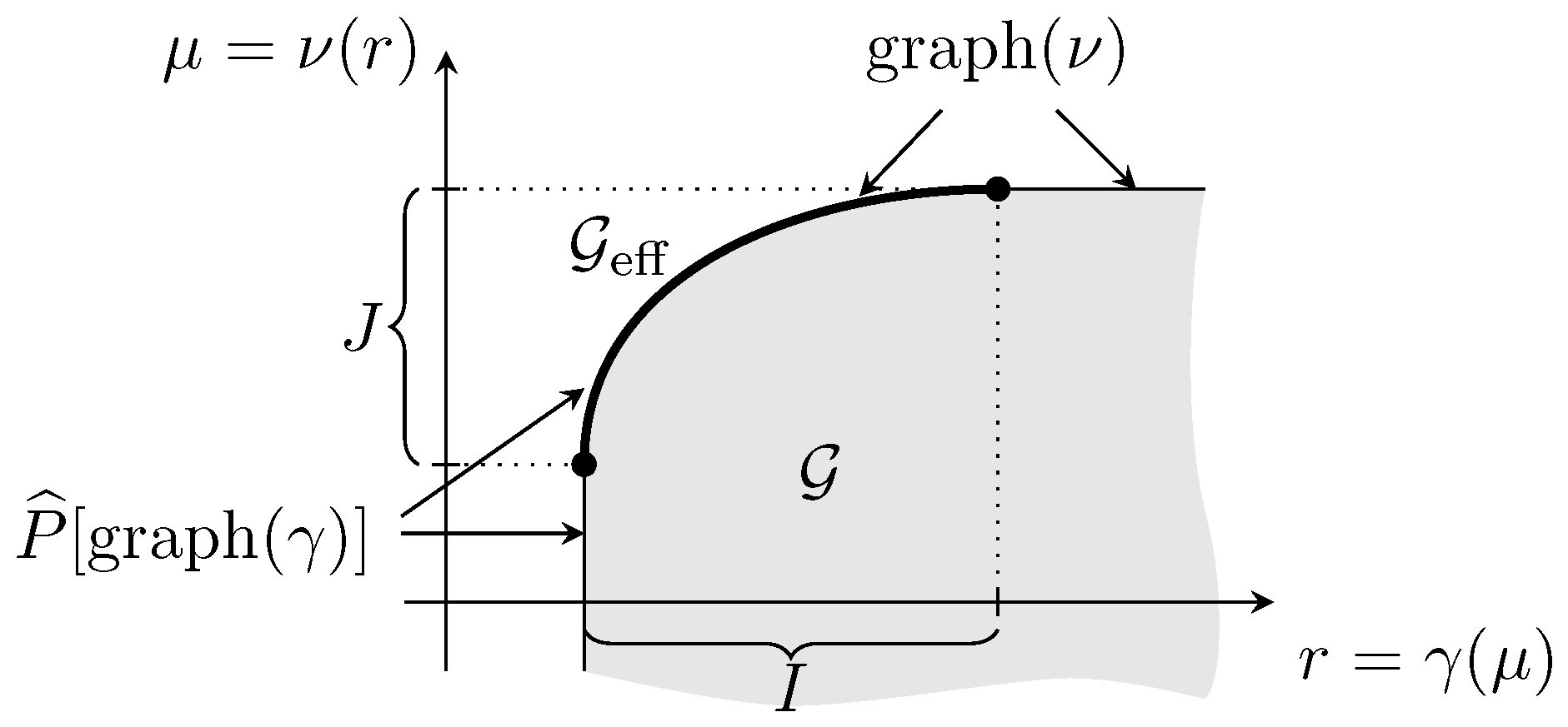
A typical situation of Theorem 2 may be viewed in
Figure 1, where
I and
J are both bounded and closed. Notice that, in this example, the graph of
and
do not coincide.
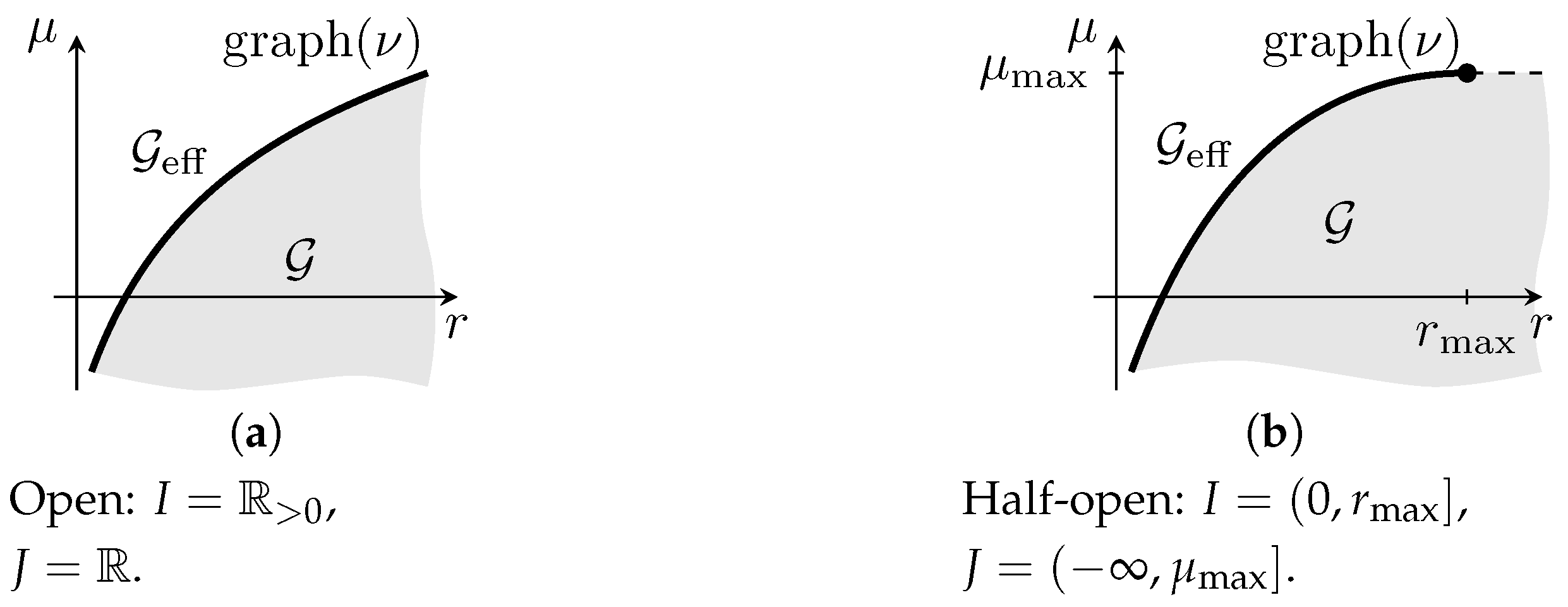
However, the intervals
I and
J may also be open, or half-open to either side (cf.
Figure 2).
With the “endpoints” of I and J being included or not, it appears that there should be at least sixteen different possibilities for the tuple , and thus for . In reality, however, we will see in Corollary 4(e) that there are only four different options for concerning the endpoints of I and J.
4. Efficient Portfolios within the General Framework of Portfolio Theory for Scalar Risk
Having investigated the efficient frontier in detail in
Section 3, we now turn our focus to related efficient portfolios granted within the GFPT.
Theorem 3 (Continuous efficient portfolio map;
Maier-Paape et al. 2023, Theorem 2.79)
. Assume, for a set of admissible portfolios, as well as for extended-valued risk and utility functions and , that Assumption 4 holds. Suppose additionally that either is strictly concave on , i.e., (u2s)
in Assumption 2 holds, or is strictly convex on , i.e., (r2s)
in Assumption 1 holds. Then, the following holds true:- (a)
Each point , with from Definition 4, corresponds to a unique efficient portfolio realizing the risk–utility values .
- (b)
The mappingis injective and continuous (one-sided continuous at finite endpoint(s) of ). Therefore, the efficient portfolios lie on a continuous curve with no self-intersections. Furthermore, X is surjective onto the set of efficient portfolios in A. - (c)
Moreover, efficient portfolios have the continuous representationsandon intervals I and J defined in (13) and (14), respectively, where ν and γ are defined in (12) and (11).
Under the standing assumptions from Assumption 4, a direct consequence of Definition 4 is that the existence part in Theorem 3(a) is obvious. Uniqueness, however, follows from the strictness conditions of either or .
Apparently, with Theorem 3, all efficient portfolios lie on a (path-connected) curve. This is essential for applications. It guarantees that little changes in
for the minimum risk optimization problem
lead to minor adaptions of the corresponding efficient portfolio solving (
18) (cf. the representation (
17), as well as the continuity of
due to Theorem 2(a), and the continuity of
X on
due to Theorem 3(b)). Thus, fund managers are able to adjust such strategies continuously. A similar remark applies to the efficient portfolios solving the maximum utility optimization problem for given
, i.e.,
For illustration purposes, we give a simple example.
Example 2 (Case of an efficient pure bond portfolio realizing minimum risk)
. Let and satisfy the assumptions of Theorem 3. Furthermore, should satisfy (r1n)
from Assumption 1 and A should contain only portfolios with unit initial cost (see Definition A4 in Appendix A). Then, the set contains exactly one element, which is the pure bond portfolio
with a minimal possible risk value . In the case where its utility value is finite, then is in fact an efficient portfolio, so that . Hence, . Following on from Proposition 2(c), we briefly explain here how to find an efficient portfolio for a given point , whose risk is not higher than r and whose utility is not lower than .
Lemma 1 (Construction of an efficient portfolio)
. Let the situation of Proposition 2 be given. Furthermore, let . Then, there exists an efficient portfolio , such that Proof. The proof of this lemma goes back to ideas provided in the proof of
Maier-Paape et al. (
2023), Proposition 2.68(c). Because of its importance, we here give the following quick argument: Since
,
follows. Then, by lowering
r and increasing
, while staying in
, one finally reaches a point
, which cannot be improved, so
results. This is a consequence of
for all
and
for all
, according to Proposition 2(b). By construction,
and
is valid, and, since
, there exists an efficient portfolio
such that
as claimed. □
5. Endpoints of the Efficient Frontier within the General Framework of Portfolio Theory for Scalar Risk
Apparently, the sets
I and
J, defined in Corollary 1, are of great interest for this theory, since they may be used for parameterizations of the efficient frontier (see Theorem 2) and the efficient portfolios (cf. (
16) and (
17)). In this section, we investigate the “endpoints” of these intervals (cf. Corollary 3).
Definition 5 (“Endpoints” of I and J;
Maier-Paape et al. 2023, Definition 2.81)
. For the intervals and , defined in (13) and (14) as projections of to the axes, we set: The above defined values may or may not lie in
, because
I or
J might be unbounded. Notice that all above representations are evident using the definitions in (
13) and (
14), as well as Corollary 1(a) and (b). The next proposition, however, is a bit more involved (cf.
Maier-Paape et al. 2023).
Proposition 3 (Alternative representations of “endpoints” of I and J;
Maier-Paape et al. 2023, Proposition 2.82)
. Assume, for a set of admissible portfolios, as well as extended-valued risk and utility functions and , that Assumption 4 holds. Then, using , the following holds true: With these representations at hand, and using some technical argumentation, it is possible to show several nontrivial relations between and on the one hand, and between and on the other hand (see below).
Corollary 4 (“Endpoint” properties;
Maier-Paape et al. 2023, Corollary 2.83)
. In the situation of Proposition 3 with and , defined in (13) and (14), we have:- (a)
, if and only if .
- (b)
If , then and .
- (c)
, if and only if .
- (d)
If , then and .
- (e)
- (i)
If and , then and .
- (ii)
If and , then and .
- (iii)
If and , then and .
- (iv)
If and , then and .
In particular, as already noted at the end of
Section 3, according to Corollary 4(e), we obtain only four different possibilities for the tuple
, and thus for
.
Thus,
Maier-Paape et al. (
2023) have examined the behavior and properties of
and
on
J and
I, respectively, (cf., e.g., Theorem 2) as well as the intervals
J and
I themselves (cf., e.g., Corollary 4) in detail. We will conclude with a brief look at how
and
behave outside
J and
I, respectively (cf.
Figure 1 for an illustration). Although the respective graphs outside
J and
I do not contribute to the efficient frontier, the behavior of
and
there is often of technical value.
Lemma 2 (Behavior of
or
outside of
J or
I)
. In the situation of Proposition 3, with and defined in (13) and (14), the following holds:- (a)
If , then and for all .
- (b)
If , then and for all .
- (c)
- (i)
If , then for all .
- (ii)
If and , then for all .
- (d)
- (i)
If , then for all .
- (ii)
If and , then for all .
Proof. We only have to consider (a) and (c) because (b) and (d) are symmetric statements.
ad(a). Let
. Then, by Corollary 4(c), (d),
with
follows. Furthermore, since
holds, and
is increasing by Proposition 2(b), we obtain
for all
.
ad(c). These assertions can be shown straight forwardly with the help of Lemma 1 by using the definitions of
in (
20) and of
in (
12). □
6. Generalizations of the General Framework of Portfolio Theory for Vector Risk
In this section, the risk function is assumed to be vector-valued, while the utility function remains to be scalar and, as before,
is a set of admissible portfolios. The results of the General Framework of Portfolio Theory (GFPT) for this case are taken from
Maier-Paape et al. (
2023, chap. 3). However, in contrast to the theory developed there for
dimensional risk vectors, we restrain ourselves here for simplicity and visualization reasons to
.
Assumption 5 (Conditions on the vector risk functions; see Assumption 1 and
Maier-Paape et al. 2023, Assumption 3.1)
. Consider a vector risk function , with lower semi-continuous components and , where is a set of admissible portfolios according to Definition 2. We say that:- (a)
satisfies one (or more) of the conditions (r1), (r1n), or (r2) if and satisfy (r1), (r1n), or (r2) from Assumption 1, respectively;
- (b)
satisfies (r2s) if or satisfies (r2s) from Assumption 1.
In the following we simplify notation by using ≤ and ≥ componentwise; i.e., for two vectors , we have , if and only if for (analogously for the other operator).
Remark 2 (Risk–utility as row vectors; see
Maier-Paape et al. 2023, Remark 3.3)
. Here, and in the following, it is convenient to have risk vectors as row vectors. Similarly, the risk–utility vectors are assumed to be row vectors, which is in contrast to our portfolio vectors , which are always column vectors. Similarly to Assumption 3, for the scalar risk case, we rely here on compactness assumptions as well.
Assumption 6 (Compact level sets in vector risk case; see
Maier-Paape et al. 2023, Assumption 3.4)
. We assume for a vector-valued risk function , as in Assumption 5, and a scalar-valued utility function , as in Assumption 2, that:- (a)
;
- (b)
For all , the setsare compact.
The next proposition lifts Proposition 1 to the vector risk case.
Proposition 4 (Properties of
; cf.
Maier-Paape et al. 2023, Proposition 3.6)
. Assume that is a set of admissible portfolios, as in Definition 2. In addition, assume that the vector risk function satisfies (r2)
in Assumption 5, and the utility function satisfies (u2)
in Assumption 2. We then have:- (a)
The set of valid risk and utility valuesis convex. - (b)
implies that, for any , we have and .
- (c)
Assume furthermore that Assumption 6(b) holds. Then, is closed.
With all that notation at hand, we can now define efficient portfolios and the efficient frontier in the vector risk case.
Definition 6 (Efficient portfolios in vector risk case; see
Maier-Paape et al. 2023, Definition 3.7)
. We say that a portfolio with finite risk and utility values is Pareto efficient
(for given vector risk function , scalar utility function , and admissible portfolios A), provided that there does not exist any portfolio such that eitherorholds. For better understanding, it is worthwhile to compare Definition 6 with the one of the scalar risk case; see Definition 3.
Definition 7 (Efficient frontier in vector risk case; see Definition 4 and
Maier-Paape et al. 2023, Definition 3.8)
. We call the set of (risk–utility) images of all efficient portfolios in the three-dimensional risk–utility space the efficient frontier
, and denote it by . Similarly to some of the properties of the efficient frontier for the scalar risk case given in Theorem 1, we obtain the following for the vector risk case.
Theorem 4 (Efficient frontier properties in vector risk case; confer Theorem 3.9 in
Maier-Paape et al. 2023)
. Efficient portfolios represented in the three-dimensional risk–utility space are all located on the boundary of the set . In case the boundary of contains a line segment parallel to any of the three coordinate axes, on such a line segment lies, at most, one efficient portfolio. The analog of the “standing” Assumption 4 for the scalar risk case is given for the vector risk case next.
Assumption 7 (Standing assumptions for efficient trade-off in vector risk case; see
Maier-Paape et al. 2023, Assumption 3.11)
. We assume the following properties:- (a)
is a set of admissible portfolios, according to Definition 2.
- (b)
is a lower semi-continuous extended-valued vector risk function satisfying (r2) in Assumption 5.
- (c)
is an upper semi-continuous extended-valued scalar utility function satisfying (u2) in Assumption 2.
- (d)
Assumption 6 concerning compact level sets holds for , and .
From now on, we use the following notations for risk values
:
i.e., we have
.
While we only had two auxiliary functions and for the scalar risk case (see Proposition 2), we now obtain three auxiliary functions for two-dimensional vector risk.
Proposition 5 (Auxiliary functions related to the efficient frontier in vector risk case; see
Maier-Paape et al. 2023, Proposition 3.12)
. Assume, for a set of admissible portfolios, as well as for extended-valued vector risk and scalar utility functions and , that Assumption 7 holds. Then, the following holds true:- (a)
.
- (b)
The functions , defined byand , defined byfor , are well-defined extended-valued functions. Moreover, the function is decreasing in , increasing in μ, and lower semi-continuous as well as proper convex. The function ν is increasing (coordinate-wise), upper semi-continuous, and proper concave. - (c)
.
In the following, using the definitions in (
26), we define the projections
for
and
as well as some kind of permutation mappings
for
.
We now shift our focus to projections of the efficient frontier
from the three-dimensional risk–utility space to planes built by two of the three variables
. This result is along the lines of Corollary 1 and Theorem 2(c) for the scalar risk case. In particular, the definitions in (
32) and (
35) below should be compared with the definitions of the sets
I and
J in (
13) and (
14).
Theorem 5 (Representation of efficient frontier in vector risk case; see Theorem 3.14 in
Maier-Paape et al. 2023)
. Assume, for a set of admissible portfolios, that the vector risk function and the scalar utility function satisfy Assumption 7. Then, the following holds true:- (a)
- (b)
For arbitrary but fixed , we set
Note that Equations (
34) and (
36) provide representations of
as graphs of the auxiliary functions
and
, respectively. In particular, we clearly obtain from (
34) and (
36) that
but also that the following holds true using, e.g., (
33) and (
34):
This can also be seen in the following example which we provide for illustration purposes.
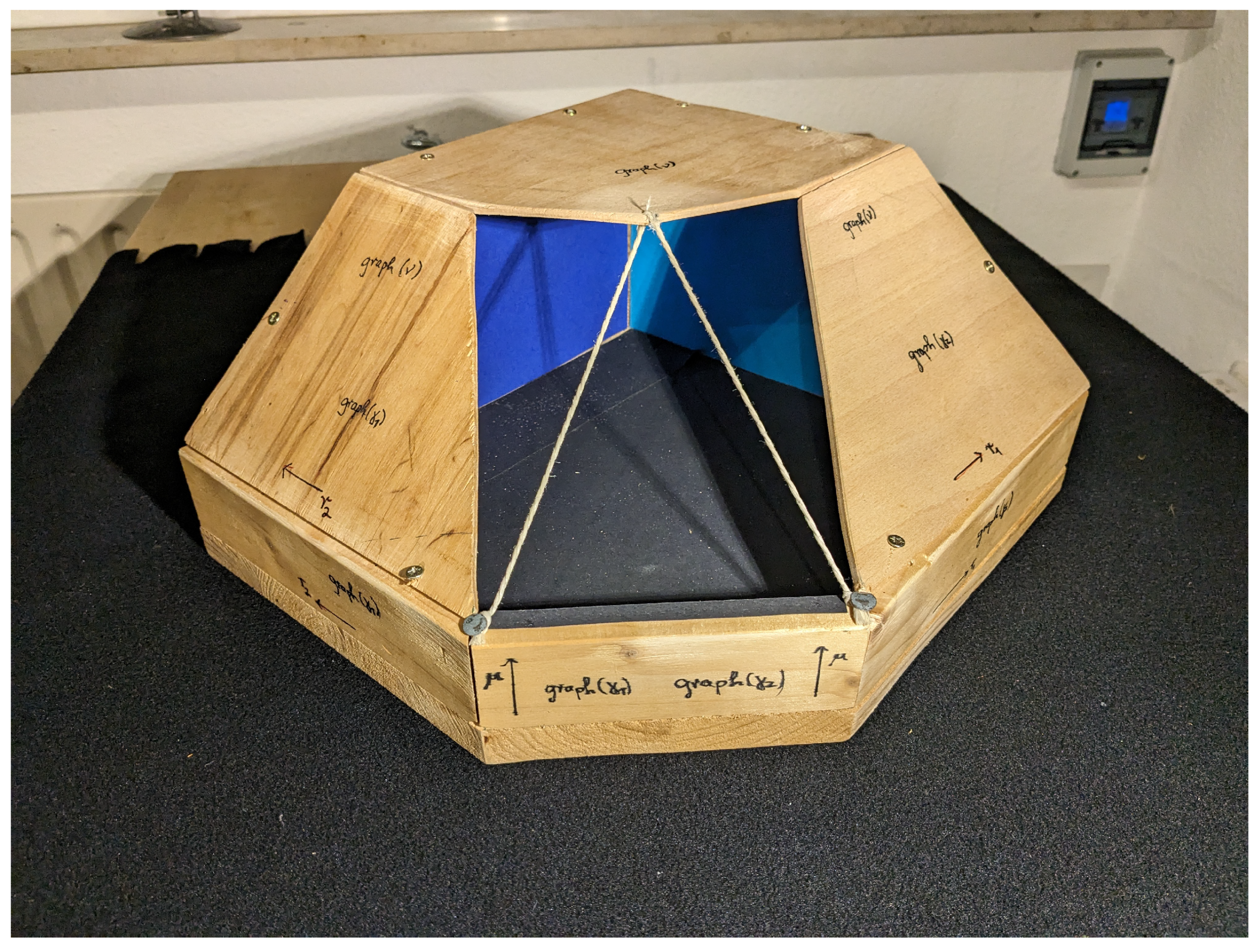
Example 3 (Non-convex projections of
)
. In Figure 3, we see a wooden model to illustrate the boundary of a possible set and its efficient frontier for the vector risk case and some fixed risk and utility functions, and , as well as a fixed set of possible admissible portfolios (whose specific forms are all irrelevant for now).Of course, the black “ground plate” of the wooden model in Figure 3 is just there to hold the construction. The extensions of the side lines of the ground plate to the left and to the right should be viewed as - and -axis. Perpendicular to these axes and upwards directed is the μ-axis. Note that, e.g., the facets on top or to the right and to the left have to be extended in - and/or -direction to to obtain all of . Similarly, the facets below are to be extended in μ-direction to . Also, the three transparent facets in front mimicked by a cord are part of . In fact, it is easy to see that only these three cord facets build . Moreover, the reader should be able to imagine, for this example, the set , i.e., the projection of to the -plane, which is a path-connected set, but is not convex in the case. This is remarkable because it is in contrast to the scalar risk case, where the projections of the efficient frontier to the axes, i.e., the sets I and J from (13) and (14) are always convex (see Corollary 3). It should be furthermore noted that the representations of
in (
34) and (
36) are an analog of Theorem 2(c) for the vector risk case. An analog of Theorem 2(b) for the vector risk case holds as well (see (
38) and (
39) below). However, continuity of
and
is no longer granted unconditionally, although, for scalar risk, this was no problem (see Theorem 2(a)).
In consensus with definition (
26), in the following, we use the convention that
followed by
is to be interpreted as a completed vector in
, i.e.,
for
.
Theorem 6 (Representation of efficient frontier 2 in the vector risk case; see
Maier-Paape et al. 2023, Corollary 3.15)
. Under the same assumptions as in Theorem 5, the following holds true:- (a)
is strictly increasing in each component; is strictly increasing in μ and strictly decreasing in (coordinate-wise) for .
- (b)
and are inverse to each other in the following sense: - (c)
and are (for fixed ) inverse to each other in the following sense:
Remark 3 (Continuity of
and
in the interior of their domains)
. As provided in Proposition 5, ν is upper semi-continuous and concave, and is lower semi-continuous and convex for . At least in the (relative) interior of their domains, both ν and are even continuous (cf. Rockafellar 1972, Theorem 10.1). Nevertheless, discontinuities on the boundary are possible (see Maier-Paape et al. 2023, Example 3.16, for a counterexample to continuity at the boundary). Path-connectedness of the efficient frontier in the scalar risk case was already not completely obvious (cf. Corollary 2). For the vector risk case, however, path-connectedness turns out to be a really subtle question. For that result, a few more assumptions are necessary.
Assumption 8 (Standing assumptions for connectedness in the vector risk case; see
Maier-Paape et al. 2023, Assumption 3.27)
. Assume for a set of admissible portfolios (cf. Definition 2) that the vector risk function and the scalar utility function satisfy Assumption 7. In particular, Assumption 6, concerning compact level sets, holds as well. We assume furthermore:- (a)
The components of the risk vector are all non-negative, i.e., , for .
- (b)
Either (r2s) holds for all (see Assumption 1), or satisfies (u2s) in Assumption 2.
With this relatively strong assumption, the path-connectedness of
follows from a quite lengthy geometric proof (cf.
Maier-Paape et al. 2023, sct. 3.2).
Theorem 7 (Path-connected efficient frontier in vector risk case; see Corollary 3.41 as well as Remark 3.29 from
Maier-Paape et al. 2023)
. Let Assumption 8 hold true, and let the components be continuous on . Then, the set is path-connected. Finally, we report results on the uniqueness of efficient portfolios and properties of the efficient portfolio map (cf. Theorem 3 for the scalar risk case).
Theorem 8 (Uniqueness of efficient portfolios for the vector risk–utility trade-off; see
Maier-Paape et al. 2023, Theorem 3.46)
. Let Assumption 7 be satisfied. Denote by the set of efficient portfolios corresponding to . Then, is an upper semi-continuous multifunction (cf. Definition A2 in Appendix A) on its domain .In addition, suppose that either the vector risk function satisfies (r2s) in Assumption 5, or the scalar utility function satisfies condition (u2s) in Assumption 2. Then, is single-valued and continuous. In particular, is also injective.
Theorem 9 (Topological properties of the efficient portfolio set; see Corollary 3.47 in
Maier-Paape et al. 2023)
. In the situation of Theorem 5 and Theorem 7, the sets from (32) and , from (35) are path-connected. Furthermore, the efficient portfolio map , from Theorem 8 is continuous in this situation and, thus, the set of efficient portfolios is path-connected as well. Moreover, the efficient portfolios can be parameterized as a graph over or , respectively, i.e., bothandyield all efficient portfolios for given , and A. Thus, according to Remark 3, and are continuous in the relative interior of N and for , respectively. Having the path-connectedness of
at hand, it is again worthwhile to note that this enables fund managers to adjust their strategies continuously, at least when parameters from the relative interior of
or
are used. The corresponding optimization problems to find efficient portfolios are similar to (
18) and (
19): firstly, the maximum utility problem
and, secondly, the two minimum risk optimization problems
In conclusion, although the notation and proofs are a bit more involved for the vector risk case, many of the results for scalar risk remain valid for the vector risk case as well.


