Trading Option Portfolios Using Expected Profit and Expected Loss Metrics

Abstract

When trading in the call and put contracts of option chains, the portfolios of strikes must be selected. The trader must also decide whether to take long or short positions at the selected strikes. Dynamic strategies for making these decisions are discussed in this paper. On any day, the strategies estimate the drift and volatility parameters of the future probability distribution of the price of the underlying asset. From this distribution, the trader can further estimate the future expected profit and expected loss that may be experienced for any portfolio of strikes of the call and put contracts. Expected profit and expected loss are the reward and risk metrics of such portfolios. An optimal portfolio can then be selected by making the reward as high as possible under the risk tolerance set by the trader. Extensive back-testing applications to historical data of SPY option chains illustrate the effectiveness of these strategies, particularly when dealing with short-term expiry options and when acting as a seller of put and call options.

1. Introduction

Traders in financial assets regularly need to decide when to take long or short positions in the assets and how large the positions should be. Technical analyses provide some guidance on such decisions. It analyzes the charts of past price movements and interprets their patterns to arrive at possible future movements and corresponding possible trades. The inherent assumption here is that past patterns are predictive of what will happen in the future. This may often be questionable. Another possible approach uses statistical time series models. This approach fits models such as autoregressive time processes to historical price data, predicting possible future prices from the models and base trading rules on the predicted prices. This approach also suffers from the drawback that it is backward-looking in terms of model calibration. When past prices are the only data source involved in trading decisions, this backward-looking drawback is present to some degree.

If options are traded with the given asset as underlying, then additional data in the form of option prices at different strikes are available. This may help to make better trading decisions. Possible future movements of the price of the underlying asset have important consequences for participants in option markets. They have strong incentives to foresee such movements. In the event that they are successful, it may be anticipated that the option prices they set contain information relevant to future price movements. In terms of measures, such as risk and conditional value at risk, the work reported by Barone-Adesi et al. (2018) supports this anticipation. Here, our challenge is rather different, namely, how to extract and exploit information from option prices to enable dynamic trading in the portfolios of option strikes that can achieve cumulative trading profits over time while simultaneously controlling trading risk.

The issue of extracting useful information from option price data has received some attention in the literature, and we review it briefly here. Among the earliest papers are those of Ross (1976), Banz and Miller (1978), and Breeden and Litzenberger (1978). Working in the no-arbitrage framework of the Black and Scholes (1973) formulas for option pricing, Breeden and Litzenberger (1978) showed that the state price density of the underlying asset price can be expressed as the second derivative of the call option price with respect to the strike price. This result suggests an estimate of the state price density which may be helpful when predicting price movements probabilistically. But statistical technical problems arose when estimating the second derivate of the call option price from discretely observed call strike prices. These problems were treated in various ways, and subsequent work produced many proposals for this purpose. Bondarenko (2003), Ait-Sahalia and Lo (2000), Poon and Granger (2003), and others have reviewed and extended the resulting literature. More recent reviews and work along similar lines were conducted by Christoffersen et al. (2013), Fengler and Hin (2015), Crisóstomo and Couso (2018), and others. Particularly notable is the so-called “recovery theorem” of Ross (2015), subsequently extended by Dillschneider and Maurer (2019). Sanford (2022) reported successful applications of this theorem in several optimal asset return portfolio contexts. However, the recovery theorem was also questioned from an empirical point of view by Jackwerth and Menner (2020) as well as Zhu (2020).

As mentioned above, in this paper, we focus on trading portfolios of contracts selected from option chains, given their option price data. As far as we know, the treatment that follows has not been discussed before. Our treatment is extracting relevant information from the option price data by adapting the method of consensus implied drift and volatility estimates discussed by Venter and de Jongh (2022a). This information is used to estimate measures of risk and reward in portfolios of contracts. Optimal portfolios are then selected in terms of balancing their risk and reward measures. We used the expected loss (EL) and expected profit (EP) as risk and reward metrics. This so-called EPEL approach to trading decisions is discussed and motivated extensively by Venter and de Jongh (2022a, 2022b).

For ease of reference, we briefly review the EPEL approach. Denote the profit and loss (P&L) of a prospective trade by the random variable $X$, distributed according to a probability measure $\mathbb{P}$ and let $\mathbb{E}$ denote the expectation under $\mathbb{P}$. If $X$ > 0, the trade results in a profit. Hence, the size of the profit of the trade is the positive part of $X$, denoted by $X^{+}$ = max {$X$, 0}. Similarly, if $X$ < 0, the trade results in a loss, and the size of the loss is the negative part of $X$, denoted by $X^{-}=\mathrm{m}\mathrm{a}\mathrm{x}\{-X,0\}$. Then ${\mathbb{E}X}^{+}$ and ${\mathbb{E}X}^{-}$ are the expected profit (EP) and expected loss (EL) of the trade. They are both expressed in the same monetary terms, which makes them directly comparable and interpretable. If a trade has an EL that is much smaller than its EP, it is an attractive trade. If the EL and EP of a trade satisfy the risk constraint ${\mathbb{E}X}^{-}\le \lambda {\mathbb{E}X}^{+}$, then it is acceptable to a trader operating at a risk tolerance level $\lambda$. Here, $\lambda$ is a number between 0 and 1. If the risk constraint only holds for $\lambda >1$, then the risk of the trade may be larger than its reward. This is typically unattractive to a trader, hence the restriction $\lambda \le 1$. A trader with $\lambda$ just below 1 may be described as risk-tolerant, whereas a trader with a smaller $\lambda$ is less risk-tolerant (or more risk-averse). The risk constraint ${\mathbb{E}X}^{-}\le \lambda {\mathbb{E}X}^{+}$ can be written in terms of the risk-to-reward ratio in the form ${\mathbb{E}X}^{-}/{\mathbb{E}X}^{+}\le \lambda$. A trader operating at a risk tolerance level $\lambda$, looks for trades that have a risk-to-reward ratio below $\lambda$.

The remainder of this paper is organized as follows. Section 2 introduces the notation used here. It contains the detailed expressions and relations required for this application of the EPEL methodology. It also shows that decisions on optimal call and/or put portfolios can be formulated and solved via mixed integer linear programming (MILP). This solution depends on the drift and volatility parameters of the geometric Brownian motion model $GBM(\mu ,\sigma )$ used to model the price movement of the underlying asset. Section 3 deals with the estimation of these parameters using option price data, thus constituting the information extraction aspect mentioned above. Section 4 gives an extensive illustration of the EPEL methodology based on back-testing using historical data of SPY option chains over the period January 2022 to June 2023. Section 5 concludes the paper with an interpretation of the results and a listing of open research opportunities. The major contribution of our paper is that the use of the EPEL methodology enables effective option trading.

2. Selecting Long or Short Call or Put Option Portfolios

Consider an asset and assume that a chain of call and put options trade with the asset as an underlying instrument. Denote the price of the asset at the end of some day $t$ by $S_t$ and the strikes of these options by $\{K_i, i=1,\dots , I$}. Further, let ${\left\{\right(C}_{b,i},C_{a,i}), i=1,\dots , I$} denote the call bid and ask option prices at the strikes, and let ${\left\{\right(P}_{b,i},P_{a,i}), i=1,\dots , I$} denote the put bid and ask prices. Also, assume the option chain will expire at the end of $h$ subsequent days.

The portfolios of options covered in this paper consist of numbers of contracts at the different strikes in which long and/or short positions in the calls and/or puts are taken. A short position at a given strike is taken by selling contracts at the bid price and a long position by buying contracts at the ask price at that strike. Denote the short-call (SC) sub-portfolio positions with ${\{N}_{b,i}, i=1,\dots , I$}, so that $N_{b,i}$ is the number of call contracts sold (or shorted) at the $i$-th strike. Similarly denote the long-call (LC) sub-portfolio positions with ${\{N}_{a,i}, i=1,\dots , I$}, the short-put (SP) sub-portfolio positions with ${\{M}_{b,i}, i=1,\dots , I$} and the long-put (LP) sub-portfolio positions with ${\{M}_{a,i}, i=1,\dots , I$}. In this section, we discuss the EPEL method used to select these portfolio positions.

Assume that the option portfolio positions taken on day $t$ are kept unchanged up to expiry on day $t+h$. On that day, the asset price is $S_{t+h}$ and when the $i$-th call expires, this gives the owner a cash flow of $\mathrm{m}\mathrm{a}\mathrm{x}(0,S_{t+h}-K_i$) per long call. Discounting back to the buying time at the rate $r$ and subtracting the buying cost, the nett P&L per long call contracts at the buying time is $\mathrm{m}\mathrm{a}\mathrm{x}(0,S_{t+h}-K_i$) $e^{-rh}-C_{a,i}$. Similarly, the nett P&L per short call is $-\mathrm{m}\mathrm{a}\mathrm{x}(0,S_{t+h}-K_i$) $e^{-rh}+C_{b,i}$. Hence, summing over all strikes, the P&L of the SC sub-portfolio is given as follows:

$$X_{SC}=-{\sum }_{i=1}^I\left[N_{b,i}\left\{\max \left(0,S_{t+h}-K_i\right)e^{-rh}-C_{b,i}\right\}\right]$$

(1)

and the P&L of the LC sub-portfolio is

$$X_{LC}={\sum }_{i=1}^I\left[N_{a,i}\left\{\max \left(0,S_{t+h}-K_i\right)e^{-rh}-C_{a,i}\right\}\right]$$

(2)

Analogously the P&L-s of the SP and LP sub-portfolios are

$$X_{SP}=-{\sum }_{i=1}^I\left[M_{b,i}\left\{\max \left(0,K_i-S_{t+h}\right)e^{-rh}-P_{b,i}\right\}\right]$$

(3)

and

$$X_{LP}={\sum }_{i=1}^I\left[M_{a,i}\left\{\max \left(0,K_i-S_{t+h}\right)e^{-rh}-P_{a,i}\right\}\right]$$

(4)

Adding these four P&L-s, the total portfolio P&L is

$$Z=X_{SC}+X_{LC}+X_{SP}+X_{LP}$$

(5)

Some constraints on the portfolio position variables must be taken into account. Denote the available volumes of the call contracts at the bid and ask prices by ${\left\{\right(V}_{b,i},V_{a,i}), i=1,\dots , I$} and those of the put contracts by ${\left\{\right(W}_{b,i},W_{a,i}), i=1,\dots , I$}. The position numbers will be integers that must be at least 0 and at most equal to the volumes available, i.e., for $i=1,\dots , I$ we used the constraints

$$0\le N_{b,i}\le V_{b,i}, 0\le N_{a,i}\le V_{a,i}, 0\le M_{b,i}\le W_{b,i}, 0\le M_{a,i}\le W_{a,i}.$$

(6)

We assume that the trader has a capital budget of the amount $A$ to trade with and portions of this budget may be used for the sub-portfolios. For the SC sub-portfolio, the trader receives the amount ${\sum }_{i=1}^I{N}_{b,i}{C}_{b,i}$ when shorting the relevant contracts. This is an exposure that may be lost eventually, should not be too large, and must form part of the overall budget. The capital outlay to buy the contracts of the LC sub-portfolio is ${\sum }_{i=1}^I{N}_{a,i}{C}_{a,i},$ and this, too, forms part of the overall capital budget. Similarly, for the SP and LP sub-portfolios, the budget constraints can be written as

$${\sum }_{i=1}^I{\{N}_{b,i}{C}_{b,i}+N_{a,i}{C}_{a,i}+M_{b,i}{P}_{b,i}+M_{a,i}{P}_{a,i}\}\le A$$

(7)

The EPEL approach entails choosing the position variables to maximize the expected total P&L (EP&L) of the portfolio, subject to the requirement that the EL/EP ratio is below a specified risk tolerance level $\lambda$. This amounts to

$$\mathrm{Maximizing} \mathrm{the} \mathbb{E}Z \mathrm{subject} \mathrm{to} \mathbb{E}{Z}^{-}\le \lambda \mathbb{E}{Z}^{+},$$

(8)

as well as the subject to the constraints (6) and (7).

To calculate the expectations here, we use the $GBM\left(\mu ,\sigma \right)$–model for the asset price’s movement. Under this model, we can write

$$S_{t+h}=S_{t+h}\left(U\right)=S_t\mathrm{e}\mathrm{x}\mathrm{p}(\left(\mu -{\sigma }^2/2\right)h+\sigma \sqrt{h}U)$$

(9)

where the random variable $U$ is $N\left(0,1\right)$–distributed. This expression can be substituted into (1)–(4) to express the P&L as functions of $U$, and then (5) can be expressed as

$$Z\left(U\right)=X_{SC}\left(U\right)+X_{LC}\left(U\right)+X_{SP}\left(U\right)+X_{LP}\left(U\right).$$

(10)

In this notation, we wish to maximize $\mathbb{E}Z\left(U\right)$ subject to $\mathbb{E}{Z\left(U\right)}^{-}\le \lambda \mathbb{E}{Z\left(U\right)}^{+}$. The integrands of these expectations must be multiplied by the unit of normal density and integrated to meet the expectations involved in (8). This turns out to be quite complicated, and the optimization problem becomes highly multi-dimensional and non-linear. Here, the discretization of the normal distribution enables great simplification, turning the entire optimization problem into a mixed integer linear programming (MILP) problem. The discretization of Venter and de Jongh (2022a) will be used. In essence this is a much-simplified version of the approach detailed in Taboga (2016). For ease of reference, it is summarized in Appendix A of this paper. The discretization amounts to replacing the continuous unit normal distribution for $U$ by a uniform discrete distribution over a set of mass points $\left\{u_d, d=1,\dots ,D\right\}$, which is chosen such that the discrete distribution closely approximates a unit of normal distribution. To apply it, let

$$s_d=S_t\exp [\left(\mu -{\sigma }^2/2\right)h+\sigma \sqrt{h}{u}_d] \mathrm{f}\mathrm{o}\mathrm{r} d=1,\dots ,D .$$

(11)

Substituting into (10) gives

$$z_d=Z\left(u_d\right)=X_{SC}\left(u_d\right)+X_{LC}\left(u_d\right)+X_{SP}\left(u_d\right)+X_{LP}\left(u_d\right)$$

$$=x_{SC,d}+x_{LC,d}+x_{SP,d}+x_{LP,d}$$

(12)

where

$$x_{SC,d}=-{\sum }_{i=1}^I\left[N_{b,i}\left\{\max \left(0,s_d-K_i\right)e^{-rh}-C_{b,i}\right\}\right]$$

$$x_{LC,d}={\sum }_{i=1}^I\left[N_{a,i}\left\{\max \left(0,s_d-K_i\right)e^{-rh}-C_{a,i}\right\}\right]$$

$$x_{SP,d}=-{\sum }_{i=1}^I\left[M_{b,i}\left\{\max \left(0,K_i-s_d\right)e^{-rh}-P_{b,i}\right\}\right]$$

$$x_{LP,d}={\sum }_{i=1}^I\left[M_{a,i}\left\{\max \left(0,K_i-s_d\right)e^{-rh}-P_{a,i}\right\}\right]$$

(13)

Define

$$z_d^{+}=\mathrm{m}\mathrm{a}\mathrm{x}\left(0, z_d\right)\hspace{1em}\mathrm{and}\hspace{1em}{z}_d^{-}=\mathrm{m}\mathrm{a}\mathrm{x}\left(0, {-z}_d\right)\hspace{1em}\mathrm{so} \mathrm{that} z_d=z_d^{+}-z_d^{-}$$

(14)

Then, the discrete version of problem (8) is as follows:

$$\mathrm{maximize} {\displaystyle \frac{1}{D}}{\sum }_{d=1}^D{z}_d\hspace{1em}\mathrm{subject} \mathrm{to} {\displaystyle \frac{1}{D}}{\sum }_{d=1}^D{z}_d^{-}\le \lambda {\displaystyle \frac{1}{D}}{\sum }_{d=1}^D{z}_d^{+}.$$

(15)

The sets of variables of interest at this stage are the position variables ${\left\{\right(N}_{b,i},N_{a,i},M_{b,i},M_{a,i}), i=1,\dots , I$} and the positive and negative parts of the overall P&L $\left\{{(z}_d^{+},z_d^{-}), d=1,\dots ,D\right\}$. They are linearly related by (13) and (14) and linearly constrained by (6) and (7). The objective function in (15) is also linear, implying that the discrete approximation turns the optimization problem into a MILP problem.

In addition to the considerations above, the trader may wish to have control over the number of strikes within each sub-portfolio to which capital is allocated and undertake this in an optimal way. To enable such control, four sets of new {0, 1} variables, ${\left\{\right(J}_{SC,i},J_{LC,i},J_{SP,i},J_{LP,i}), i=1,\dots , I$} can be introduced, taking the value 0 if nothing is to be allocated at the relevant strike and 1 otherwise. Then, it is required that

$$\begin{gathered} N_{b,i}{C}_{b,i}\le A{J}_{SC,i}, N_{a,i}{C}_{a,i}\le A{J}_{LC,i}, \\ {M}_{b,i}{P}_{b,i}\le A{J}_{SP,i},\hspace{1em}{M}_{a,i}{P}_{a,i}\le A{J}_{LP,i},\hspace{1em}for i=1,\dots , I \end{gathered}$$

(16)

and if the constraints are added,

$$\begin{gathered} {\sum }_{i=1}^I{J}_{SC,i}\le {Num}_{SC}, {\sum }_{i=1}^I{J}_{LC,i}\le {Num}_{LC}, \\ {\sum }_{i=1}^I{J}_{SP,i}\le {Num}_{SP}\hspace{1em}\mathrm{and}\hspace{1em}{\sum }_{i=1}^I{J}_{LP,i}\le {Num}_{LP}, \end{gathered}$$

(17)

then the number of strikes in the sub-portfolios can be limited to prespecified values ${Num}_{SC}, {Num}_{LC}, {Num}_{SP}$ and ${Num}_{LP}$. For example, if ${Num}_{SC}={Num}_{LC}={Num}_{SP}={Num}_{LP}=1$, then capital should be allocated to at most one strike in each sub-portfolio. Note that these additional constraints on the number of strikes are all linear so that the MILP solution method can still be used.

The trader may also be interested in the EP and EL of individual trades at each possible strike in the sub-portfolios. Taking all position variables as 0, except for $N_{b,i}$ which is taken as one, $Z$ becomes equal to $X_{SC,i}=\left\{C_{b,i}-\max \left(0,S_{t+h}-K_i\right)e^{-rh}\right\}$. For this individual SC trade at the $i$-th strike only, the EP and EL are given by

$$\begin{gathered} {EP}_{SC,i}=\mathbb{E}{\left\{C_{b,i}-\max \left(0,S_{t+h}-K_i\right)e^{-rh}\right\}}^{+}\hspace{1em}\mathrm{and} \\ {EL}_{SC,i}=\mathbb{E}{\left\{C_{b,i}-\max \left(0,S_{t+h}-K_i\right)e^{-rh}\right\}}^{-}. \end{gathered}$$

(18)

The ratio ${EL}_{SC,i}/{EP}_{SC,i}$ serves as a metric of the quality of this individual trade. Using the discrete normal approximation, the expressions in (18) can be approximated by

$$\begin{gathered} {EP}_{SC,i}={\displaystyle \frac{1}{D}}{\sum }_{d=1}^D{\left\{C_{b,i}-\max \left(0,s_d-K_i\right)e^{-rh}\right\}}^{+}\hspace{1em}\mathrm{and} \\ {EL}_{SC,i}={\displaystyle \frac{1}{D}}{\sum }_{d=1}^D{\left\{C_{b,i}-\max \left(0,s_d-K_i\right)e^{-rh}\right\}}^{-}\hspace{1em}\mathrm{respectively}. \end{gathered}$$

(19)

This is similar for LC, SP, and LP individual trades.

This completes the description of the EPEL method applied to options trading portfolio selection, except for one aspect, namely that $s_d$ in (11) depends on the (unknown) values of the parameters $\mu$ and $\sigma$ in the $GBM\left(\mu ,\sigma \right)$–model for the price process of the underlying asset. The calculations above can only be carried out once suitable estimates of these parameters are obtained. This is where the extraction of information from the option prices comes in, and we attend to this in the next section.

3. Estimating the Drift and Volatility Parameters

Here, we describe the estimation of the parameters of the $GBM\left(\mu ,\sigma \right)$–model needed for $s_d$ in (12). This is conducted by an adaptation of the method of consensus-implied estimates discussed by Venter and de Jongh (2022a).

The discounted cash flow at time t of the call contract at the $i$-th strike is max{0, $e^{-rh}\left(S_{t+h}-K_i\right)\}$. Under the $GBM\left(\mu ,\sigma \right)$–model for the asset price, the expectation of this cash flow is given by Equation (6.2) by Venter and de Jongh (2022a). Adjusted to the notation here and using (9), this becomes

$$C_i\left(\mu ,\sigma \right){=e}^{-rh}{\int }_{b_i}^{\infty }{(S}_t{e}^{\left(\mu -{\sigma }^2/2\right)h+\sigma \sqrt{h}u}-K_i)\phi (u)du$$

$$=S_t{e}^{\left(\mu -r\right)h}\left[1-\mathsf{\Phi }\left(b_i-\sigma \sqrt{h}\right)\right]-K_i{e}^{-rT}\mathsf{\Phi }\left(-b_i\right)$$

(20)

with $b_i=\left\{\mathrm{l}\mathrm{o}\mathrm{g}(K_i/S_t)-\left(\mu -{\sigma }^2/2\right)h\right\}/\sigma \sqrt{h}$. Similarly, the discounted cash flow at time t of the put contract at the $i$-th strike is max{0, $e^{-rh}\left(K_i-S_{t+h}\right)\}$ and under the $GBM\left(\mu ,\sigma \right)$–model, the expectation of this cash flow is

$$P_i\left(\mu ,\sigma \right){=e}^{-rh}{\int }_{-\infty }^{b_i}{(K_i-S}_t{e}^{\left(\mu -{\sigma }^2/2\right)h+\sigma \sqrt{h}u})\phi (u)du$$

$$=-S_t{e}^{\left(\mu -r\right)T}\mathsf{\Phi }\left(b_i-\sigma \sqrt{T}\right)+K_i{e}^{-rT}\mathsf{\Phi }\left(b_i\right)$$

(21)

Venter and de Jongh’s (2022a) estimates are composed of $\mu$ and $\sigma$ which are chosen to minimize the weighted sum of squared differences over strikes between the “observed” prices and their expected counterparts under the $GBM\left(\mu ,\sigma \right)-$model. However, for both calls and puts, we had two “observed” prices, namely the bid and ask prices. We took a combination of the bid and ask prices to compare against the expected counterparts. The matching criterion was then given by

$$\begin{gathered} SSD\left(\mu ,\sigma ,\eta \right)={\sum }_{i=1}^I{w_i\{\left[\eta C_{b,i}+\left(1-\eta \right)C_{a,i}-C_i\left(\mu ,\sigma \right)\right]}^2+ \\ {\left[\eta P_{b,i}+\left(1-\eta \right)P_{a,i}-P_i\left(\mu ,\sigma \right)\right]}^2\} \end{gathered}$$

(22)

where $\eta$ is the combination parameter. Then, this criterion was minimized over the three parameters $\mu ,\sigma ,\eta$. The resulting estimates of $\mu$ and $\sigma$ were denoted by ${\widehat{\mu }}_t$ and ${\widehat{\sigma }}_t$, respectively. A suitable choice for the weights $w_i$ at the different strikes in (22) is

$$w_i=\mathrm{e}\mathrm{x}\mathrm{p}(-f\left|K_i-S_t\right|)/{\sum }_{j=1}^I\mathrm{e}\mathrm{x}\mathrm{p}(-f\left|K_j-S_t\right|)$$

(23)

where $f>0$ is a tuning constant. This places more weight on the strikes near to the money (i.e., near to the current price of the underlying asset). The tuning constant can be chosen to control the extent of the weight concentration near the money. Other possible weight choices may be the trade volumes or open interests at the strikes, normalized to a sum of one. Thus, the differences at the strikes with high volume-wise market attention count more than those at strikes with lower attention, a reasonable consideration to apply. For any possible choice of weights, the minimization problem to obtain ${\widehat{\mu }}_t$ and ${\widehat{\sigma }}_t$ can be handled using a non-linear programming solver.

These estimates constitute the information on price drift and volatility extracted from the option data. As noted previously, to the extent that the option market participants are forward-looking in their price settings, these estimates may be assumed to be relevant to subsequent price movements, at least in the near future. Under this assumption, we can substitute ${\widehat{\mu }}_t$ and ${\widehat{\sigma }}_t$ into Equation (11) and then solve the MILP problems to obtain explicit predictions and judgments of the optimal portfolio position variables. In the next sections, we explore the effectiveness of this trading method by back-testing, using empirical option price data.

4. Empirical Illustration When Trading SPY Option Chains

In this section, we illustrate the EPEL option trading strategy explained above. Back-testing is performed, using historical SPY option chain data obtained from the CBOE data shop (see CBOE (2023)). These data cover the period from 3 January 22 to 30 June 23. For each trading day and all active option chains, it contains the daily strikes together with the bid-ask prices and volumes of contracts at the strikes, both for calls and for puts at 15:45 pm and at the end of the trading day.

The detailed back-testing results are presented in an extensive Excel file, linked as SPY Results Aug 24. This file provides Supplementary Material to this paper. It contains fifteen spreadsheets showing the important stages and findings of this back-testing study. Extracts from these spreadsheets are incorporated and discussed in this section of the paper.

Sheet 1: 4 January 22 Cons Ests. As stated above, we anticipate that information extracted from past option data will only be useful for near-term trading. Therefore, the back-testing will focus on options with one day to expiry, i.e., with $h=1$. In view of this very short term, we take the interest rate as $r=0$. Until further notice, we will work with end-of-day (EOD) data. The first sheet is entitled ‘4 January 22 Cons Ests’. It serves to illustrate the option data used and the consensus estimation step to obtain ${\widehat{\mu }}_2$ and ${\widehat{\sigma }}_2$ for day 2, as explained above in Section 3. We chose 4 January 22 since this is the first trading day with an option chain expiring one day forward. The illustration uses normalized weights as in (23) above with the tuning constant $f=0.5$. Under these weights, strikes outside the range from 460 to 500 play an insignificant role, and the data of such strikes are effectively dropped. Column A shows the strikes used, and columns B to E show the corresponding closing bid-ask call and put option prices. The weights are in column F. With these data, the non-linear programming solver NLPQN in PROC IML of SAS delivers the minimizing consensus values of ${\widehat{\mu }}_2=-0.00038$ and ${\widehat{\sigma }}_2=0.00638$ and the combination parameter estimate $\widehat{\eta }=0.5$. The latter implies that we are effectively working with mid-bid-ask prices, as shown in columns G and I. Columns H and J show the corresponding fitted expected call and put prices from Equations (20) and (21). Clearly, observed and fitted prices agree well. The drift and volatility parameter estimates can be used as inputs into the EPEL formulas and calculations for 4 January 22.

Sheet 2: 4 January 22 EPEL metrics. This sheet provides an illustration of the individual trades at each possible strike, as discussed at the end of Section 2. It has four blocks, each showing the EP, EL, and the EL/EP ratio estimated by the equations in (19). For example, if the trader contemplates selling one call contract at strike 474 with a price of 3.60, the expected profit (EP) would be 1.13, and the expected loss (EL) would be 1.10; the EL/EP ratio is 0.98, which would mean that the trader operates at a high-risk tolerance level with this trade. In contrast to this, there is the possible trade of selling one put contract at strike 472 with a price of 0.13. It has an EP of 0.13, EL of 0.04, and a ratio of 0.33; therefore, the trader will be operating at a low-risk tolerance level. Thus, this possible trade on its own does appear attractive.

Sheet 3: P&L-s Lam one. Moving on to the portfolio back-testing process itself, calculations for the consensus drift and volatility parameter estimates were performed every day, and the results were applied in the EPEL portfolio context, as explained in Section 2. We started by assuming that the trader was risk-tolerant and set $\lambda =1$. Also, until further notice, we assumed that the trader selected at most one contract per sub-portfolio on each trading day. In terms of the parameters in Section 2, this meant that ${Num}_{SC}={Num}_{LC}={Num}_{SP}={Num}_{LP}=1$. Sheet 3 provides back-testing results under these trading assumptions. Columns A and B show the dates and numbers of the trading days. Column C shows the closing price of SPY on the days, and column D shows the number of days to expiry for the option chain with the nearest time to expiry. Columns E to H show the realized P&L-s for each of the sub-portfolios when executing the EPEL rules, and column I show their sum. Trading reflected by non-zero entries occur only on days where expiry is only one day away. Moreover, no trading in some sub-portfolios may occur on a trading day (see, e.g., E8 and H8). Columns K to O show the accumulated P&L over days. Graphs of the cumulative P&L-s over time are displayed in the sheet; we return to them below.

Sheet 4: Trades Lam one. More details on the portfolio trades are shown in Sheet 4. For example, on the second day, the entries in the long calls columns I, J, and K show that 956 call contracts were bought at strike 480 and at the price of 0.28 per contract. This entailed a capital allocation of 267.68 for that trade. The close price of SPY on the next trading day (5 January 22, column C5) was 468.38. Since this was below the strike of 480, the long call expired worthlessly, and the trade yielded a loss of the capital employed, i.e., the P&L of this trade was −267.68. This is the entry shown in the “P&L-s Lam one” sheet for 4 January 22 in column F3. As another example, in the “Trades Lam one” sheet, the entries in columns Q, R, and S for 4 January 22 show that 31 put contracts at strike 479 were bought at the price of 2.20 each. This entailed a capital allocation of 68.20 for that trade. As shown above, the close price of SPY on the next trading day was 468.38, which is 10.62 below the strike of 479. Hence, this trade delivered a profit of 31 × (10.62 − 2.20) = 261.02. This is the entry in column H3 of the sheet “P&L-s Lam one”. This is similar to the other trades recorded in the sheet “Trades Lam one”.

Another short put trade that produced a very poor result was on 17 May 22, day number 94. Columns M, N, O, and P show that 609 contracts at strike 401 were sold at the price of 0.47 each. The next day, SPY closed at 391.86, which was 9.14 below the strike of 401. Consequently, that trade delivered a loss of 609 × (9.14 − 0.47) = 5280.03. We will return to this trade again when discussing Sheet 9 below.

Note that for the sake of simplicity, the P&L-s of trades are recorded against the day when the trade was executed, although the actual money flow may occur only at the end of the next day. Since the interest rate is taken as zero, this convention makes no difference to the results reported here.

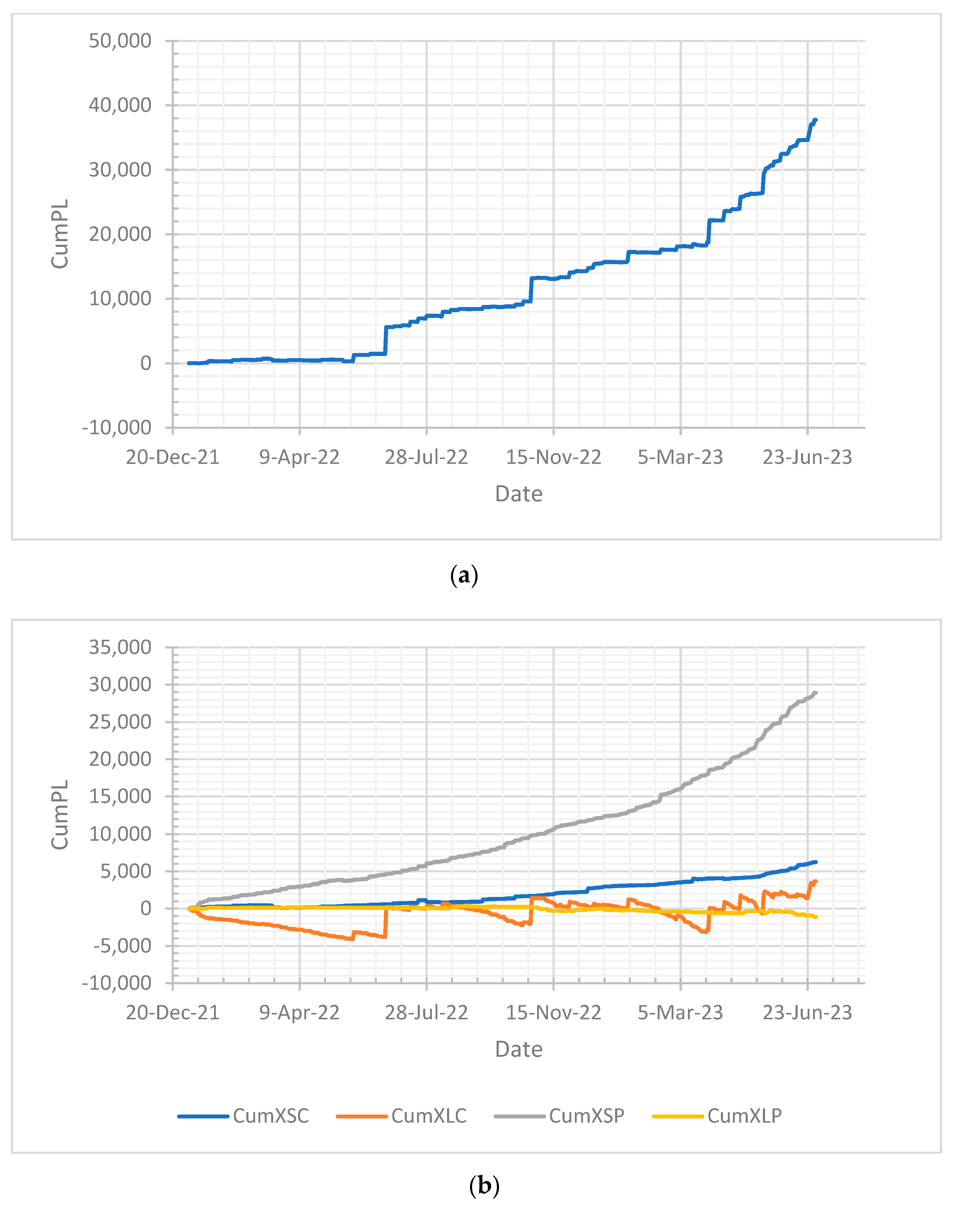
Returning to the sheet “P&L-s Lam one”, its graphs are extracted in Figure 1 below. The top panel shows the graph for the total portfolio cumulative P&L-s over time, and the bottom panel shows the graphs of the four sub-portfolio cumulative P&L-s. Over the first seven months of this period, the portfolio total did not show a definite trend, but after that, the EPEL rules performed very well in terms of producing a steadily growing cumulative total P&L. Relatively large drawdowns occurred (e.g., at the start of trading and also on 17 May 22, which is the trade referred to above) but apart from these, the total P&L grew quite consistently over time. From the bottom panel, it is evident that the short-put (SP) sub-portfolio was the major contributor to this performance. The two long sub-portfolios performed rather poorly.

Sheet 5: Realized Stats Lam one. This sheet tables and compares empirical versions of the EPEL trade metrics. The calculations are performed for the P&L-s produced over time in the back-testing process rather than from daily GBM assumptions—hence the term “Realized Stats”. This table is repeated here as

Table 1. Trade statistics of sub-portfolios compared.

Realized Trading Stats	SC	LC	SP	LP	Total
Number of profit events	176	34	211	49	120
Number of loss events	24	180	4	99	95
% profit events	88.00	15.89	98.14	33.11	55.81
% loss events	12.00	84.11	1.86	66.89	44.19
Ave profit size per profit event	88.39	1236.19	193.06	200.20	594.17
Ave loss size per loss event	334.98	206.79	3622.54	139.48	386.60
Ave profit size per trade day	77.80	196.42	189.47	66.31	331.64
Ave loss size per trade day	40.22	173.94	67.41	93.32	170.84
Realized Risk to Reward ratio	0.52	0.89	0.36	1.41	0.52
Ave PL per trade	37.59	22.47	122.07	−27.02	160.80
Ave Capital used per trade	137.81	206.68	194.10	177.48	650.18

below. The second and third lines of the table show the numbers of trades that resulted in profit and loss, respectively. The fourth and fifth lines express these frequencies in percentage terms and may be interpreted as the empirical estimates of the probabilities of profitable and losing trades, respectively. In these frequency terms, the two short sub-portfolios outperformed the two long sub-portfolios substantially. Lines six and seven show the average sizes of the profit and loss events. In contrast to the frequency terms, in size terms, the two long sub-portfolios performed better than the two short ones. The size and frequency terms are combined into one metric by taking their products; the results are shown in lines nine and ten, and their ratios are in line 11. These metrics may be thought of as empirical realized estimates of the EP, EL, and EL/EP ratio of the EPEL method. The results confirm again that the SP sub-portfolio was best, with the realized risk-to-reward ratio quite low at 0.36, followed by SC (0.52), LC (0.89), and LP (1.41). These numerical findings are in line with the impression conveyed by the graphs in the bottom panel of Figure 1. The last two lines of Table 1 show the average P&L per trade and the average size of the capital involved per trade over the period. Here, the SP sub-portfolio delivered the remarkable result of producing about 122 units of profit per trade, involving only 194 units of capital outlay.

Sheets 6–8: P&L-s Lam half, quart, eighth. Thus, far back-testing was performed when trading under the maximal risk tolerance level $\lambda =1$. Next, we look at lower risk tolerance specifications, namely $\lambda =0.5, 0.25$ and 0.125. The results are given in the sheets entitled “P&L-s Lam half”, “P&L-s Lam quart”, and “P&L-s Lam eighth”. Their layouts and contents are like those of “P&L-s Lam one”. Moving from sheet to sheet, it can be noted that as $\lambda$ becomes smaller, the EPEL rules deliver cumulative P&L results, and the graphs become less noisy, especially over the early part of the period and for the SC and SP sub-portfolios. Moreover, they tend to succeed in avoiding larger drawdowns while retaining their overall growth tendency. Thus, it is evident that smaller choices of $\lambda$ produce risk-reduced trading without seriously affecting the desirable P&L growth performance over time. Figure 2 illustrates the favorable results for the chosen $\lambda =0.125$.

Sheet 9: Trades Lam eighth. It is particularly interesting to look at the trades on 17 May 2022, which are referred to when discussing Sheet 4 above. Recall that with the choice $\lambda =1$, a large drawdown of 5134.53 occurred, mostly due to the loss of 5280.04 from the SP trade (see day 94 of “P&L-s Lam one”). Then, with the choice $\lambda =0.125$, the drawdown size was only 238.94, with 153.57 coming from the SP trade (see day 94 of “P&L-s Lam eighth”). Sheet 9 shows more details of this trade. Columns M, N, O, and P show that 1706 contracts at strike 392 were sold at the price of 0.05 each. The next day, SPY closed at 391.86, which was only 0.14 below the strike of 392. Consequently, the trade delivered a small loss of 1706 × (0.14 − 0.05) = 153.54. Thus, with the choice $\lambda =0.125$, the EPEL algorithm avoided the large drawdown experienced under the choice $\lambda =1$. Column Z of “Trades Lam eighth” shows that the prespecified EL/EP ratio of 0.125 was binding in the optimization solution. Compare this to the corresponding value of 0.4696 found during the optimization solution with the $\lambda =1$ specification (day 94 of “Trades Lam one” column Z). In that case, the trader operated with a high-risk tolerance and thought that achieving an EL/EP ratio of 0.4696 was attractive. The result was that the large draw-down that was actually experienced was not anticipated. The strike selected to trade in was too close to the money and led to a large loss. The upshot is that trading at a low-risk tolerance setting helps to avoid such large, though infrequent, losses.

Sheet 10: P&L-s 1545 data. Up to this point, we used the end-of-day (EOD) prices and volumes to find optimal EPEL allocations and assumed that the trader could execute simultaneously at closing time. From a practical point of view, this is a rather unrealistic assumption. Next, we will base the EPEL metrics on the 15:45 pm data of option prices and volumes to select the trades to be performed at EOD. Those trades will then be conducted at EOD prices and at the smallest of the optimal 15:45 volumes and the EOD volumes. Such assumptions may be more realistic from a practical point of view. The best results reported so far were obtained with the risk tolerance parameter $\lambda =0.125$, and we continue with this choice here. Moreover, trading in the two long sub-portfolios did not improve the total portfolio results, and we reported only for trading in the two short sub-portfolios, SC and SP. We still assumed that the trader might select at most one strike from each of these two sub-portfolios. Sheet 10 shows the results. 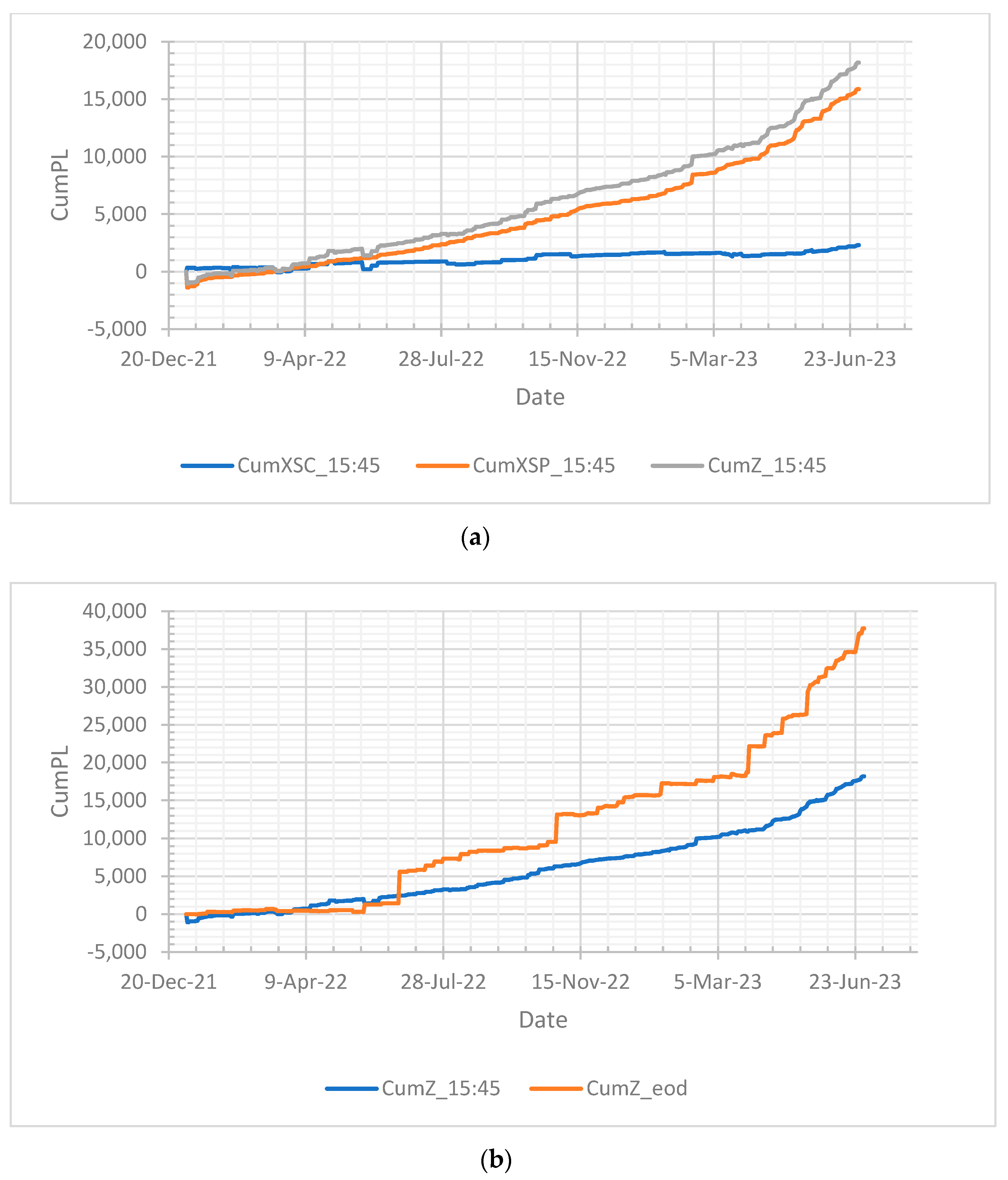Figure 3 is extracted from this sheet. Its top panel plots the cumulative P&L-s of the two short sub-portfolios, together with that of their total. The SP sub-portfolio performed much better than the SC sub-portfolio, although the latter did make consistent contributions. The bottom panel of Figure 3 compares the total portfolio P&L based on the 15:45 data with that based only on the EOD data. This suggests that using 15:45 data entails some loss of benefit since lower overall growth is obtained—likely due to making decisions somewhat earlier than what was experienced on the next trading day.

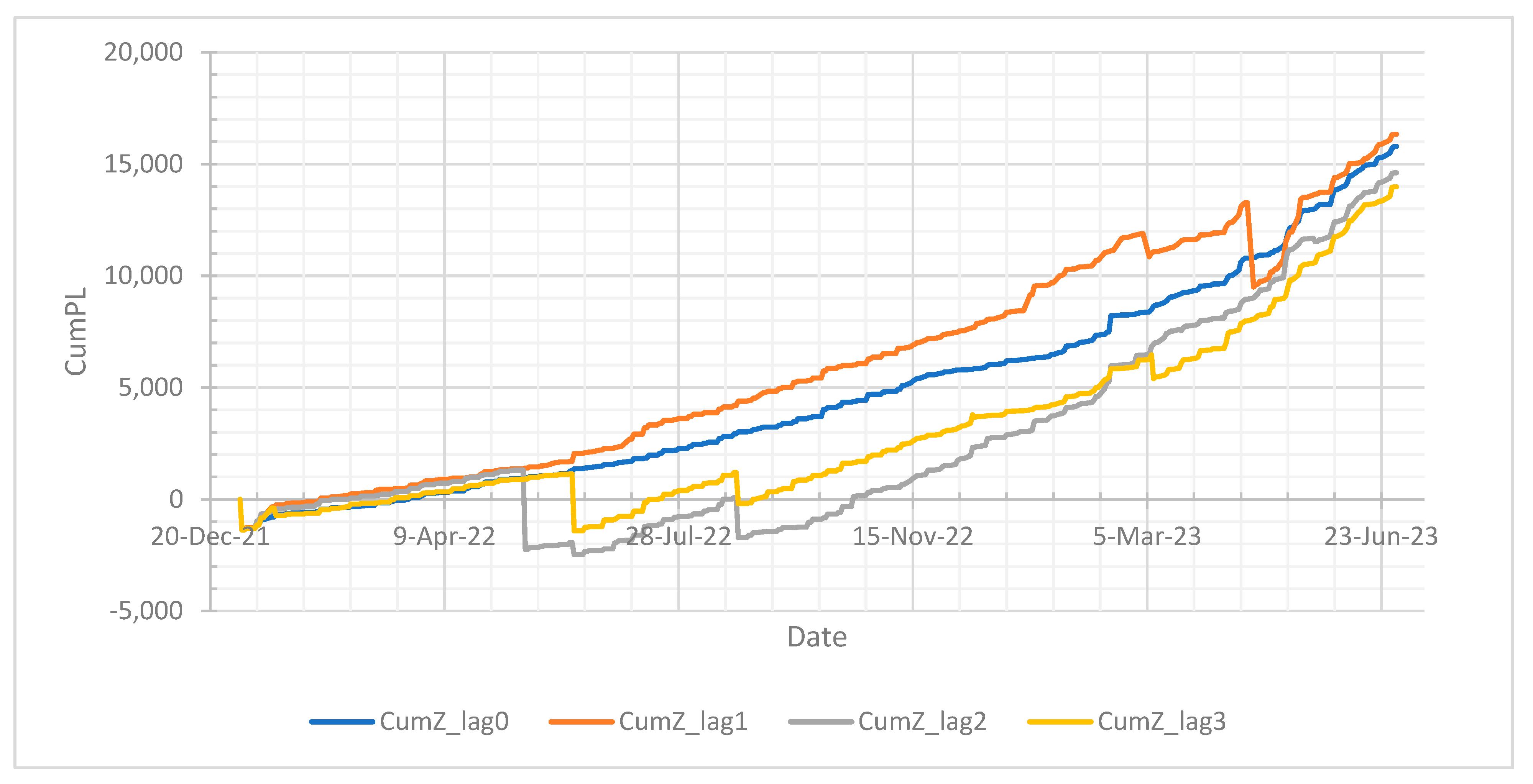
Sheet 11: Info duration. The underlying surmise of this back-testing study is that the option traders are forward-looking in their price settings, allowing us to extract estimates of the drift and volatility parameters that are useful for finding favorable future trades. The results reported so far bear out that this may be a successful strategy, but one may wonder how long such extracted information stays useful. Sheet 11 contains some results in this direction. A simple approach to shed light on the duration question is to replace the most recent drift and volatility estimates with earlier estimates and see how much difference this makes to the P&L performance. Sheet 11 uses the same settings as Sheet 10 above but focuses on the short put (SP) sub-portfolio only. It reports the cumulative P&L-s under four time-lagged choices of the drift and volatility estimates, namely 0, 1, 2, and 3 days, respectively. Figure 4 is extracted from this sheet and shows the results.

The blue curve represents the P&L growth when there is no time lag, as in the bottom panel of Figure 3. The other curves use the time-lagged drift and volatility estimates in their calculations; they still show growth over time but tend to fall prey to occasionally large drawdowns, marring their performance. The clear conclusion is that the use of the most recent option data yields the best option trading performance.

Sheet 12: P&L-s data 3 positions. Thus far, we have constrained the trader to select at most one position per sub-portfolio per day. Typically, only a small portion of the total trading capital was used under this constraint. If the performance was good under this constraint, then we could anticipate that it would be even better if more than one position per sub-portfolio was allowed since there might be favorable strikes to select near those that produced good results. Sheet 12 reports the results in this direction. Here, the assumed set-up is similar to Sheet 10; we traded in the two short portfolios but allowed positions for three strikes at most for each portfolio. 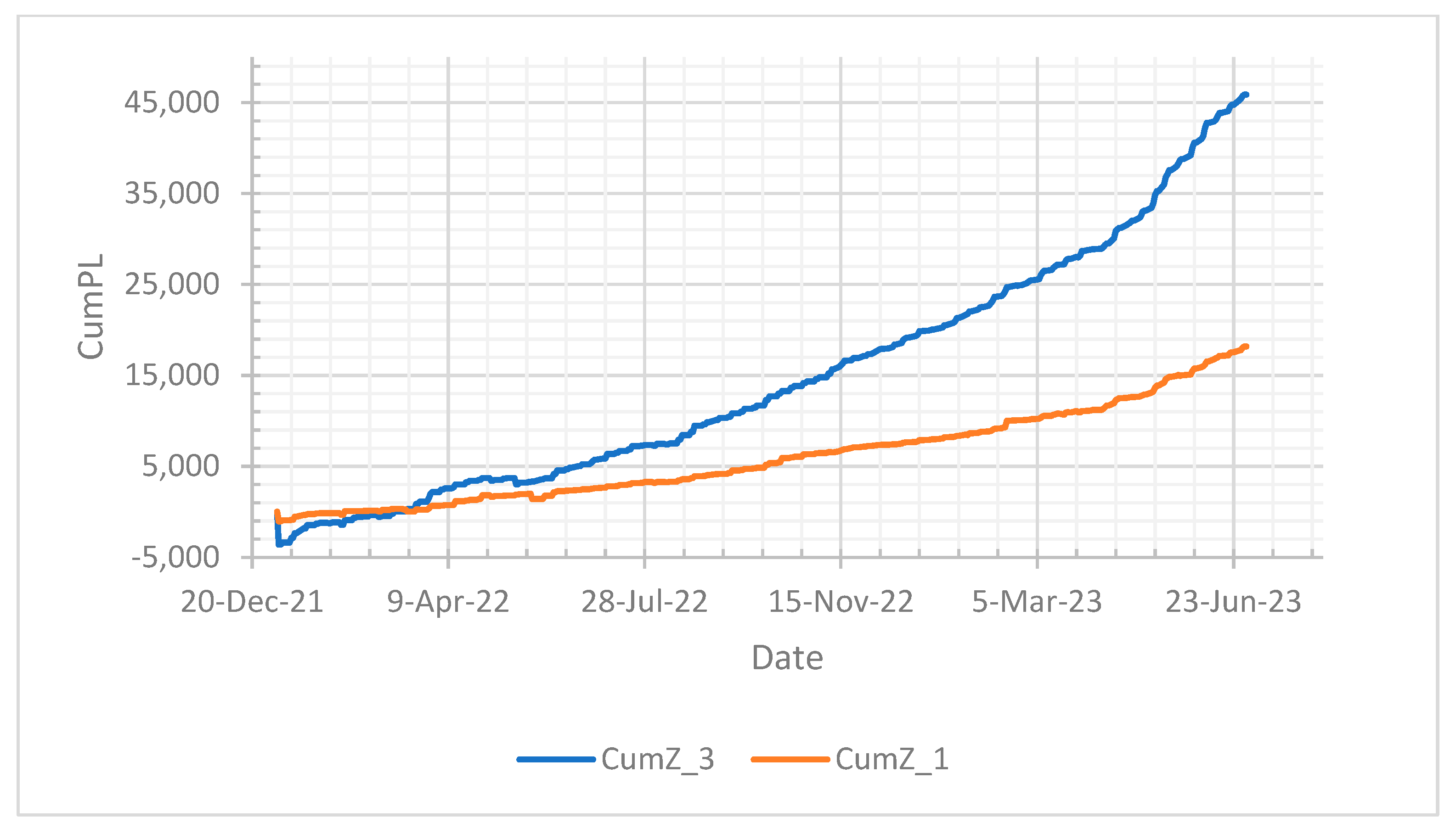Figure 5 compares the total P&L performance in this case with that under the single position constraint.

As anticipated, there was much to be gained by trading on a larger scale than with single positions only. The average capital per trade used here was 294.03 (column R line 15), with an average P&L per trade of 213.45 (column R line 14). This was more than double the results when trading with the single position constraint, namely 138.46 and 84.60 (sheet 9, column R lines 15 and 14). Moreover, with a total trading capital available of 1000, there was scope to increase the number of positions allowed substantially.

Sheet 13: Skew BM. Above, we used the GBM model for the price movements of the underlying asset. The applicability of the GBM has been questioned widely in the literature, and many distributional modifications have been proposed. A recent example is the paper by Zhu and He (2017), who reviewed this literature and discussed the skew Brownian motion (SBM) as an alternative model to use in option pricing. This model can be incorporated very easily into the context of our paper, as described in Appendix B.

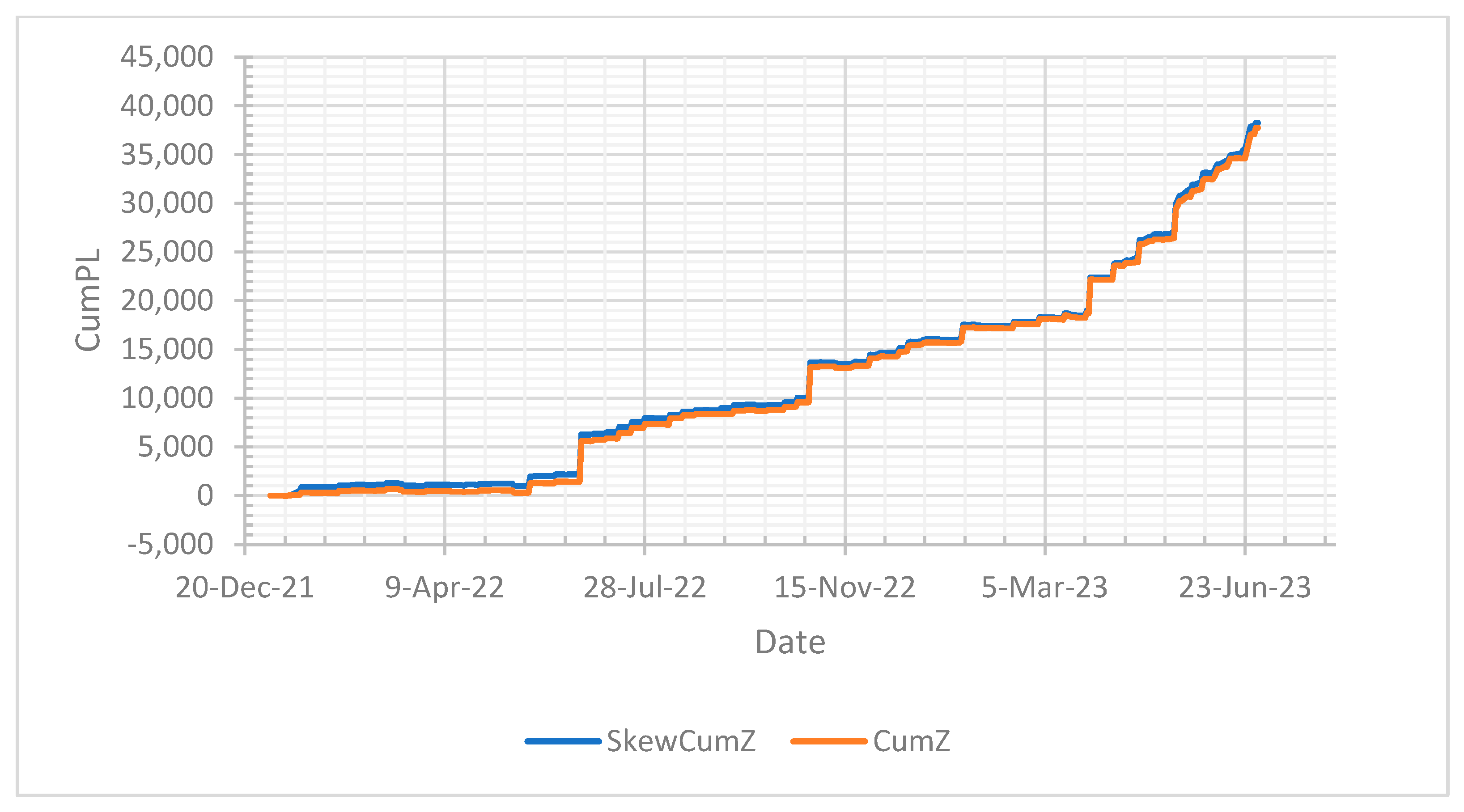
We implemented the SBM model in the back-testing process. It turns out that the consensus estimates of the skewness parameter of the SBM are practically always very close to zero, implying that the SBM model stays close to the GBM model. Sheet 13 supplies numerical results in this regard. The consequence is that the P&L performance of the EPEL trading approach does not change appreciably under this skew BM model. This is clearly demonstrated in Figure 6, which compares the P&L performance under the SBM model with that obtained under the GBM model for the settings of Sheet 8. The apparent robustness of the GBM model in our context may be due to the daily updating and re-estimation of its parameters using the newest option price data.

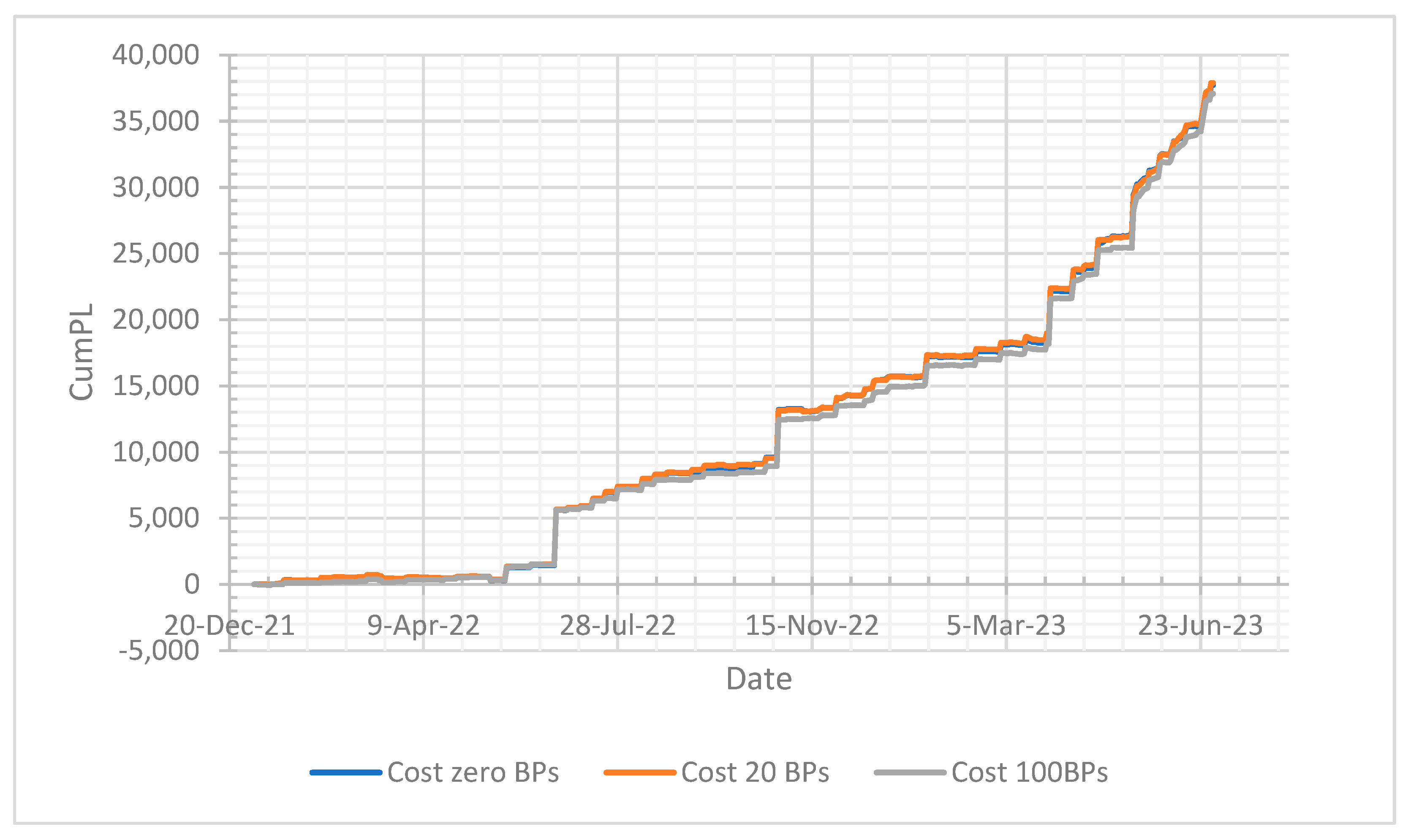
Sheet 14: Costs. For the sake of simplicity, back-testing usually starts with the zero trading costs assumption. If one cannot find profitable algorithms when the cost is zero, one would also not find profitable algorithms when the cost is not zero. The illustrative results above were obtained in this spirit. This led to favorable results such as those discussed for Sheets 8 and 9. We continued with that setting but assumed that the trader faces non-zero proportional trading costs at each buy and sell trade. We extended the formulas in Section 3 to accommodate this cost assumption. Sheet 14 shows the cumulative P&L-s over time for two cost levels, namely 20 and 100 basis points. Figure 7 exhibits a graph of the results. As one would anticipate, non-zero costs slow down the P&L growth over time, but not severely, even under the very high 100 basis points assumption.

Sheet 15: Discretization. In all the results above, $D$ = 201 mass points were used for the discretization of the normal distribution. We found that increasing this number did not lead to a much different P&L performance. This is illustrated in Sheet 15. The same setting as in Sheet 14 was used, and the cumulative P&L-s were calculated both with $D$ = 201 and $D$ = 501 for the number of mass points. The latter set of calculations involved handling much larger matrices in the MILP optimization program and thus required much more computer time. Figure 8 exhibits a graph of the results. Clearly, the greater computational effort is not worthwhile.

5. Conclusions

This paper deals with extracting information from option chain data and using it to trade algorithmically in option chains. The information extracted consists of daily estimates of the drift and volatility of the price of the asset underlying the option chain. These are used, in turn, to estimate the expected profit and loss of the possible long and short portfolios of call and put options at various strikes and with one day to expiry. Optimal portfolios are then estimated in terms of balancing expected profit and expected loss and satisfying relevant constraints. This methodology was extensively back-tested using SPY option chain data. Some important conclusions and interpretations of the results obtained from this EPEL study are given as follows.

Back-testing dynamic trading requires assumptions tailored to the available data. This may cause inherent limitations on the general validity of the results. Nevertheless, the results reported strongly suggest that option traders can profit substantially from executing a short put option portfolio daily that has a low risk-to-reward ratio in terms of expected loss and profit metrics. That this is a reasonable finding can be explained as follows. In principle, selling an option delivers an immediate premium income to the seller. In the case of selling a put option, if strikes are selected so that the price of the underlying asset stays above them up to expiry, then the seller can retain the full premium as profit and have no loss-producing obligations. To make this outcome likely, the strikes selected must be far below the money at execution time. But the strikes selected must also not be so far below that the premium is very small. The EPEL methodology succeeds well in balancing these two conflicting requirements, resulting in the consistent accumulation of profit over time.

Similar arguments can be made for short-call option portfolios. If the strikes are selected such that the price of the underlying asset stays below them up to expiry, then the seller will also retain the full premium as profit. Again, the strikes should not be selected so far above the money at execution that the premium is very small. The back-testing results also confirm that the EPEL methodology succeeds in this regard, but not to the same extent as with short put trading. This difference between the two short portfolios may be due to an asymmetry between reasons for trading in put and call options. To be able to sell a put option. a willing buyer of the put is needed; such a buyer may wish to hedge against a perceived threat to an existing investment in the underlying asset. To be able to sell a call option, a willing buyer of the call is also needed, but now the buyer likely perceives an opportunity to participate in a possible price rise of the underlying asset. Acting on a perceived threat is quite different from acting on a perceived opportunity, implying that the market of buyers of put options is likely larger than the market of buyers of call options. This difference is clearly visible in the different P&L performances of the two short options portfolios found in the back-testing study. It is also in line with the so-called prospect theory of Kahneman and Tversky (1979) and Kahneman et al. (1982).

The two long portfolios performed poorly overall. Perhaps the overriding factor here is the very short time to expiry. While this works in the favor of the seller who has short puts and calls, the opposite applies to the buyer who takes long positions.

The work reported in this paper can be extended in many directions. Much trading in the options market is performed using compound option structures. Some examples are straddles, bull and put spreads, and many more combinations of puts and calls at different strikes, together with positions in the underlying asset. Optimal dynamic portfolios of such option structures would benefit traders greatly. There is an open opportunity to apply the EPEL methodology to calculate such structured option portfolios.