Article

Quadratic Unconstrained Binary Optimization Approach for Incorporating Solvency Capital into Portfolio Optimization

1
Department of Financial Mathematics, Fraunhofer ITWM, Fraunhofer-Platz 1, 67663 Kaiserslautern, Germany
2
DZ BANK AG, Platz der Republik, 60325 Frankfurt am Main, Germany
3
JoS QUANTUM GmbH, Platz der Einheit 2, 60327 Frankfurt Am Main, Germany
4
R+V Lebensversicherung AG, Raiffeisenplatz 2, 65189 Wiesbaden, Germany
*
Author to whom correspondence should be addressed.
Risks 2024, 12(2), 23; https://doi.org/10.3390/risks12020023
Submission received: 29 November 2023 / Revised: 25 January 2024 / Accepted: 26 January 2024 / Published: 29 January 2024
(This article belongs to the Special Issue Computational Finance and Risk Analysis in Insurance II)

Abstract

:
In this paper, we consider the inclusion of the solvency capital requirement (SCR) into portfolio optimization by the use of a quadratic proxy model. The Solvency II directive requires insurance companies to calculate their SCR based on the complete loss distribution for the upcoming year. Since this task is, in general, computationally challenging for insurance companies (and therefore, not taken into account during portfolio optimization), employing more feasible proxy models provides a potential solution to this computational difficulty. Here, we present an approach that is also suitable for future applications in quantum computing. We analyze the approximability of the solvency capital ratio in a quadratic form using machine learning techniques. This allows for an easier consideration of the SCR in the classical mean-variance analysis. In addition, it allows the problem to be formulated as a quadratic unconstrained binary optimization (QUBO), which benefits from the potential speedup of quantum computing. We provide a detailed description of our model and the translation into a QUBO. Furthermore, we investigate the performance of our approach through experimental studies.

1. Introduction

The support for strategic asset allocation is being examined, with a particular focus on incorporating capital requirements according to Solvency II into investment decisions. The goal is to investigate to what extent the use of quantum-inspired systems can contribute to better managing the complexity of the problem and delivering more stable results. Reduced fluctuations in investment portfolios contribute to the stabilization of companies and, consequently, the financial system. Similarly, methods for determining regulatory requirements can be reconsidered. More accurate calculations through adequate representation and inclusion of risk factors can lead to a more precise evaluation of risks, resulting directly in lower costs and increased efficiency.
Quantitative asset management has its origins in Modern Portfolio Theory, which was described by Harry Markowitz in 1952. In portfolio theory, the goal is to construct a portfolio with an optimal risk-return tradeoff. Markowitz’s classical theory uses volatility as a measure of risk and introduces a mathematical framework to calculate the risk and return characteristics of a portfolio based on the weights assigned to individual assets, their expected returns, their volatilities, and their correlations (Markowitz 1952). By optimizing the risk-return tradeoff, investors can construct portfolios that provide the desired level of return while minimizing risk or vice versa. In our application, we extend the above optimization framework by integrating another risk measure, the Solvency capital requirement (SCR). Finding the optimal tradeoff among these three objectives is a multi-objective optimization problem and one that is interested in finding Pareto-optimal solutions. We show how finding Pareto-optimal points in this optimization problem can be related to solving quadratic unconstrained binary optimization (QUBO) problems, for which quantum computing (especially quantum annealing) is considered a promising candidate for a significant speedup compared to traditional methods.
In the Section 1, we give a brief overview of the basic concepts of multi-objective optimization and introduce solvency capital as a further objective to be considered in portfolio optimization alongside return and volatility. Furthermore, we outline how Pareto-optimal points for this extended problem can be found using QUBOs. In the Section 2, we show in detail how to construct the required QUBO formulation. We demonstrate how the SCR is approximated by a quadratic function, how the continuous optimization variables can be replaced by binary ones and how the condition “unconstrained” is achieved. In the Section 3, we apply our approach to a real-world example from the insurance industry consisting of 26 assets and evaluate how closely the Pareto frontier has been approximated with our method.

1.1. Our Contribution

Our first contribution is that we incorporate the SCR as an objective function into portfolio optimization and we are the first to study portfolio optimization including SCR via a quantum-inspired approach. In order to tackle this problem with quantum annealing or gate-based quantum hardware, the problem has to be translated into a quadratic unconstrained binary optimization problem, thus translating continuous variables into binary, writing the budget constraint as penalty function in the objective function, and, most importantly, find a quadratic formulation of the SCR. The SCR objective is, in general, highly non-quadratic. Thus, we propose classical machine learning (general least squares regression) to find a quadratic approximation to the SCR, which is again our contribution. Our third contribution lies in the evaluation of the performance. We use a multi-objective view of the performance measurement. The hypervolume indicator has rarely been used outside the multi-objective community and in particular has never been applied to quantum algorithms. Here, we examine the solutions obtained by the QUBO using the original multi-objective formulation consisting of return, volatility, and SCR.

1.2. Multi-Objective Portfolio Optimization

At the center of Markowitz portfolio optimization lies the trade-off between risk and return, which are often considered conflicting objectives in portfolio optimization. Multi-objective optimization provides a framework to explore and analyze the trade-offs between these conflicting objectives. We start with a general discussion of the basics of multi-objective optimization and then concretize to our use case.
Let n , p N and X R n . For p 2 and i = 1 , , p let f i : X R be an arbitrary function. We write f : X R p , x ( f 1 ( x ) , , f p ( x ) ) for the vector-valued function obtained by combining the f i . A multi-objective optimization problem is defined as
min x X f ( x ) ,
and, in this case, X is called the set of feasible solutions. Since there is no total order relation on R p (like the ≤ relation on R ), the minimum is taken with respect to a partial order and, therefore, a minimal element x X is not unique, in general, see Ehrgott (2005) for more details on ordering relations. This leads to the concept of Pareto-optimality. A solution x X is Pareto-optimal if there is not a solution x ¯ X , x ¯ x with f i ( x ¯ ) f i ( x ) , i = 1 , , p and f j ( x ¯ ) < f j ( x ) for at least one j { 1 , , p } . In this case, the image y = f ( x ) is called nondominated. We call the set of all nondominated images Pareto frontier. The goal of multi-objective optimization is to determine the Pareto frontier as accurately as possible.
One of the most common approaches to solving a multi-objective problem is the weighted sum method, which transforms a multi-objective problem into a single-objective problem through a scalarization function. Given a weight vector, also known as preference vector, λ R 0 p , we solve the single-objective optimization problem
min x X λ t f ( x ) .
Note, that an optimal solution to this problem is Pareto-optimal and called supported. In general, a Pareto-optimal solution x X is not supported, that is to say, there is no λ R 0 p such that x can be realized as a solution to the single-objective problem (2). A sufficient condition for all Pareto-optimal points to be supported is the convexity of all objective functions f 1 , , f p . We refer to Halffmann et al. (2022) and Ehrgott (2005) for further introduction into multi-objective optimization.
We turn back to Markowitz’s portfolio theory and show how portfolio optimization fits into the general framework of multi-objective optimization. Let n N be the number of assets in our portfolio and R = ( R 1 , , R n ) a random vector describing the return of assets. We assume that expected values, variances and covariances are known and define
μ i : = E ( R i ) , σ i , j : = Cov ( R i , R j ) ,
for i , j = 1 , , n . These quantities are further summarized to the return vector μ : = ( μ 1 , , μ n ) and the covariance matrix Σ : = ( Cov ( R i , R j ) ) i , j { 1 , , n } . It is also assumed that any denomination of assets is permissible and that the budget is normalized to 1. Negative shares are excluded. Under these conditions, the formulation of portfolio optimization most frequently considered in the literature is given by
min μ t x + q · x t Σ x , s . t . x 1 + + x n = 1 , 0 x i 1 for each i = 1 , , n ,
where q > 0 is called the risk aversion. A vector ( x 1 , , x n ) R n that satisfies the above constraints is called an investment decision. In line with the above discussion, the problem in (3) arises when the weighted sum method is applied to the multi-objective problem (1), in which p = 2 and the objective functions are given by
f 1 : X R , x μ t x , f 2 : X R , x x t Σ x ,
and the feasible solutions as X = { x [ 0 , 1 ] n | x 1 + + x n = 1 } . The preference vector is λ = ( 1 , q ) . The traditional formulation of portfolio optimization is, therefore, a special case of the multi-objective view, whereby different risk aversion factors correspond to different points on the Pareto frontier. When extending portfolio optimization to include further objectives, the concept of Pareto-optimality provides the most natural mathematical framework for investigating trade-offs between multiple objectives.
Another reason for taking the multi-objective view is its importance for applications in industry. Decision-makers can use the Pareto frontier to explore a range of solutions, each representing a different compromise between competing objectives. This flexibility is valuable for decision-makers who want to make informed choices based on their priorities. In the following section, we will introduce a target function, which models a crucial key figure with profound implications for insurance companies.

1.3. Extension of Portfolio Optimization by Solvency Capital Requirement

Solvency capital requirement (SCR) is a term used in the insurance industry to refer to the minimum amount of capital that insurance companies are required to hold in order to ensure their solvency and financial stability. It is a regulatory measure designed to protect policyholders and ensure that insurance companies have sufficient funds to cover unexpected losses and are adequately equipped to cope with various risks such as credit risk or market risk deriving from the activities carried out.
The currently implemented SCR introduced by EIOPA, the European Insurance and Occupational Pensions Authority, in the Solvency II framework (European Commission 2015) is defined in a way that is closely related to the concept of Value at Risk or VaR in short. In general, given any random variable Z and α ( 0 , 1 ) , let
VaR Z ( α ) = inf { z R : P ( Z > z ) 1 α } .
Now let x [ 0 , 1 ] n be an investment decision and let L x be the random variable modeling the loss of the insurance company with an annual time horizon. Our notation emphasizes that the loss depends, among other things, on the company’s investment decision. The Solvency capital requirement is then defined as
SCR L D ( x ) : = VaR L x ( 0.995 ) E [ L x ] ,
where the index LD stands for loss distribution (we will introduce another variant of the SCR shortly). It can be interpreted as the amount of funds the insurance company needs to hold in order to be solvent with a probability of 0.995 in the following year. Note, that the expression VaR Z ( α ) E [ Z ] does not define a convex risk measure, so considering the SCR in an optimization problem is usually hard (see Artzner et al. (1999) for further details on risk measures).
Determining L x and its distribution is difficult as it requires sophisticated stochastic modeling as well as efficient techniques for implementing the necessary calculations (see Bauer et al. (2012) for more details). For companies that are challenged by the implementation, the supervisory authority offers a standardized method for approximating SCR L D ( x ) , without the need to calculate L x (in fact, most insurance companies in Germany calculate their solvency capital using this standardized method in order to reduce costs).
The so-called standard formula for SCR L D is intended to capture the main quantifiable risks to which most companies are exposed. In contrast to the name, the standard formula is not a single formula, but rather a framework of various calculation rules that include both, parameters calibrated by the regulator and company-specific quantities (e.g., the investment decision x). Here, we will only give a brief overview of the structure of the standard formula. For details, we refer to European Parliament and European Council (2009).
The core idea is to divide the calculation of SCR L D into several modules and aggregate them according to specific correlation assumptions. The following modules are considered:
RiskMod : = { market , health , default , life , non life , operational , intangible assets } .
The Standard formula assigns a risk value SCR i ( x ) R to each of the above risk modules i RiskMod (again by giving specific calculating rules that do not involve stochastic modeling). For the calculation of the individual SCR i ( x ) , various methodological approaches are used, which may differ from module to module. For example, for the calculation of SCR market ( x ) , it is necessary to estimate the risk for investments in equities, which is realized by a simple factor model. For this, the regulator calibrates stress factors which are multiplied by company-specific quantities. The stress factors are real numbers which, in the case of equity risk, correspond to a change in market prices according to a 200-year event. The company-specific quantity is here the amount of capital invested in equities. Similar rules are also provided for the other risk modules, for which we refer to the literature.
The individual risk modules are aggregated as follows. Using the correlation matrix Corr given by the regulator (European Parliament and European Council (2009), Annex IX, (1)), the risk modules life, non-life, health, market, default, intangible asset are amalgamated yielding the so-called Basic Solvency Capital Requirement BSCR ( x ) . To ultimately reach an approximation for the Solvency Capital Requirement SCR L D ( x ) , a twofold process is involved: first, we deduct the adjustment factor Adj representing loss-absorption capacity, and subsequently, we integrate the SCR operational element SCR operational , addressing the imperative for capital against operational risk, into the BSCR ( x ) framework. This yields the following expression:
SCR L D ( x ) BSCR ( x ) Adj + SCR operational ,
with
BSCR ( x ) = i j Corr i j SCR i ( x ) SCR j ( x ) ,
where i , j RiskMod and Corr i j denotes the correlation coefficient between them. The right-hand side of (4) is the method most frequently used in practice to calculate SCR L D . Finally, we consider the company’s own funds in relation to SCR L D . The own funds are assumed to be a positive constant and denoted as o f R . Thus, we define
SCR : R n R x o f BSCR ( x ) Adj + SCR operational
and include this function as a further objective in portfolio optimization, which is to be maximized (the denominator is always non-zero). Therefore, to summarize our general problem setting, given the objective functions
f 1 : R n R , x μ t x , f 2 : R n R , x x t Σ x , f 3 : R n R , x SCR ( x ) ,
we are interested in the Pareto frontier of the multi-objective optimization problem
min f 1 ( x 1 , , x n ) , min f 2 ( x 1 , , x n ) , min f 3 ( x 1 , , x n ) , s . t . x 1 + + x n = 1 , 0 x i 1 for each i = 1 , , n .
In the next subsection, we outline how the determination of Pareto-optimal points of (5) can be traced back to solutions of quadratic unconstrained binary optimization problems, for which quantum computing provides an essential speedup.

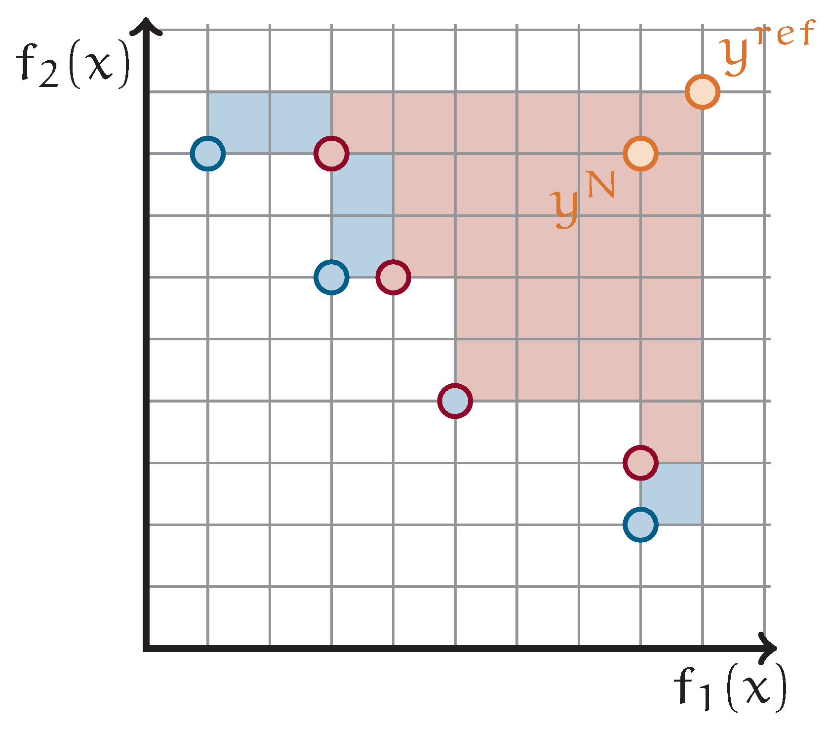
1.4. Finding Pareto-Optimal Points by Solving QUBOs

In the last subsection, we discussed the importance for insurers to extend portfolio optimization by the SCR. It is important for decision-makers in the industry to have an overview of the entire Pareto frontier to make informed choices based on their preferences.
In insurance practice, finding a good approximation to the Pareto frontier of (5) presents some difficulties, mainly due to the lack of convexity of f 3 . First, the Pareto-optimal points are not necessarily supported. This means that, from a theoretical point of view, it is not guaranteed that a good coverage of the Pareto frontier can be achieved by applying the weighted sum scalarization. However, for our particular use case, this is not a major problem in practice because the image of f = ( f 1 , f 2 , f 3 ) is still very close to a convex set. Second, even if good coverage of the Pareto frontier is possible, the lack of convexity makes the repeated application of the weighted sum method with subsequent solutions of the corresponding single-objective optimization problems (one problem for every preference vector) very costly. In the rest of this paper, we demonstrate how to reformulate this problem as a QUBO. The motivation for this is that, given a QUBO formulation, a number of different solution methods can be applied, which might eventually offer significant speedups over traditional approaches. Apart from the classical simulated annealing, one such method is quantum annealing. There are indications, that for some problems, quantum annealing may provide speedups beyond what any classical algorithm can achieve Somma et al. (2012). There already are commercially available hardware implementations for quantum annealing, even though our problem is not well suited for the current DWAVE annealer, for example, due to the large bandwidth of our QUBO matrices. This prevents the mapping of our QUBO matrices onto the hardware in an efficient way. However, our formulation might be able to utilize future generations of quantum annealing hardware.
Another possible path to follow is to employ a gate-based quantum computer. For that, the QUBO formulation makes it possible to solve the problem, for example, with the QAOA algorithm Zhou et al. (2020). All current gate-based quantum computing hardware is not able to execute quantum gates with a sufficiently low error rate to solve real-world problems. Nevertheless, the steady progress over the past few years in increasing hardware fidelities and error-correction techniques makes the availability of such hardware in the foreseeable future likely (see, for example, the roadmap published by IBM (2023)).
In the following, we will outline how to move from our original problem to a QUBO. We show step by step how to obtain the properties “quadratic”, “unconstrained” and “binary”, with the technical details being discussed in more detail in the respective subsections of Section 2. The original problem we start with is given by (5) and we want to determine the Pareto frontier as accurately as possible. For this, the weighted sum method is used (despite the lack of convexity, most of the Pareto-optimal points are supported). This leads to the single-objective, constrained, continuous optimization problem
min λ 1 f 1 ( x 1 , , x n ) + λ 2 f 2 ( x 1 , , x n ) + λ 3 f 3 ( x 1 , , x n ) s . t . x 1 + + x n = 1 0 x i 1 for each i = 1 , , n ,
with ( λ 1 , λ 2 , λ 3 ) R 0 3 . Next, we describe the transition to a quadratic objective function. By a quadratic function, we mean a polynomial with real coefficients in n variables of total degree 2 . This definition also includes linear mappings (polynomials of total degree one) and constants (polynomials of total degree zero). The functions f 1 and f 2 are already quadratic by definition. The function f 3 is not quadratic but can be well approximated by a quadratic function, as we will see in Section 2.1. We, therefore, replace f 3 with a quadratic approximation f 3 , a p p r o x (this approximation is usually not convex). With f 1 , f 2 , f 3 , a p p r o x being quadratic, the weighted sum
λ 1 f 1 + λ 2 f 2 + λ 3 f 3 , a p p r o x
is also quadratic. As an intermediate step, we have a quadratic, constrained, continuous optimization problem
min λ 1 f 1 ( x 1 , , x n ) + λ 2 f 2 ( x 1 , , x n ) + λ 3 f 3 , a p p r o x ( x 1 , , x n ) s . t . x 1 + + x n = 1 0 x i 1 for each i = 1 , , n ,
with ( λ 1 , λ 2 , λ 3 ) R 0 3 .
We now describe the transition from “continuous” to “binary”. The idea is to discretize the continuous optimization variables ( x 1 , , x n ) by replacing the domain [ 0 , 1 ] n with a well-chosen finite grid G [ 0 , 1 ] n . Writing B : = { 0 , 1 } , we consider a bijective mapping
T : ( B m ) n G
which transforms bit strings into grid points. Here, m N will be a parameter that controls the refinement of the grid and results from the fact that we approximate each variable x i by m bits. The definition of G and T will be given in Section 2.2. Our optimization problem will then take the form of a quadratic, constrained, binary problem
min λ 1 f 1 ( T ( y ) ) + λ 2 f 2 ( T ( y ) ) + λ 3 f 3 , a p p r o x ( T ( y ) ) s . t . y ( B m ) n , T ( y ) 1 + + T ( y ) n = 1 for all y ( B m ) n .
with ( λ 1 , λ 2 , λ 3 ) R 0 3 . Note, for the index notation in the last line of (8) that T ( y ) is an element of R n for every y ( B m ) n . Of course, the discretization reduces accuracy, but by increasing m, the discretization can, in principle, be made arbitrarily accurate.
The property “unconstrained” is achieved by incorporating the linear constraint into the objective function. This is obtained through the introduction of a penalty factor λ P > 0 , which associates a certain cost for violating the linear constraint (see Section 2.3). We arrive at
min λ 1 f 1 ( T ( y ) ) + λ 2 f 2 ( T ( y ) ) + λ 3 f 3 , a p p r o x ( T ( y ) ) + λ P ( T ( y ) 1 + + T ( y ) n 1 ) s . t . y ( B m ) n
with ( λ 1 , λ 2 , λ 3 , λ P ) R 0 3 × R > 0 which is a quadratic, unconstrained, binary optimization problem. The solutions here are not exactly the same as in the constrained case (8). One has to choose λ P carefully so that the solutions of (9) are not too far away from the solutions of (8). In the next section, we will describe the individual steps of this outlined procedure in more detail. In Section 3, we apply this approach to a real-world example from the insurance industry and evaluate how well the Pareto frontier can be determined by solving (9).

2. The QUBO Formulation

In this section, we will show how to formulate our extended portfolio optimization problem (5) as a Quadratic Unconstrained Binary (QUBO) optimization problem. This includes how to approximate the SCR-objective f 3 by a quadratic function, how to encode vectors containing fractions in binary code, and how to replace a linear constraint with a penalty term.
The availability of specialized hardware to solve QUBO problems, in particular, the quantum annealer developed by D-Wave, has attracted interest in the QUBO formulation in recent years. Portfolio optimization was an early example. The basic idea to formulate a Markowitz optimization as a QUBO was sketched and some toy example experiments were solved on the D-Wave quantum annealer, in Elsokkary et al. (2017). Another example that explains some aspects in more detail is Venturelli and Kondratyev (2019), which also used D-wave annealing hardware. Variations in the basic portfolio optimization have been examined, too, for example, dynamic settings, in which one optimizes the portfolio changes one makes over a period of time (Rosenberg et al. (2015)).
QUBOs are optimization problems of the form
min y B N y t Q y ,
where B = { 0 , 1 } , N N and Q R N × N . Since
y t Q y = y t Q + Q t 2 y
for all y B N , one can always assume that the matrix Q R N × N in (10) is symmetric.
It will be important for our optimization problem that the QUBO formulation can not just accommodate pure quadratic, but also linear and constant terms, i.e., the optimization problems we will be working with are of the form
min y B N y t P y + b t y + c ,
where P R N × N , b R N , and c R . Given an optimization problem of the form (11), one can always find a symmetric matrix Q R N × N such that the solution set of (10) is equal to the solution set of (11). For the constant c, this is easy to see, as the presence of a non-trivial c has no impact on the optimum at all.
To see how to accommodate the linear term, note that we can write the entries of b = ( b 1 , , b N ) on the diagonal of a diagonal matrix D = diag ( b 1 , , B N ) R N × N . Since the components of y are binary, we have y t D y = b t y . The objective function of a QUBO is, therefore, always a quadratic function in the sense of our definition from Section 1.4 (polynomial of total degree 2 ). The presentation in Section 1.4 is, therefore, consistent with this subsection.
Given many QUBOs with corresponding matrices of the same format, one can form a linear combination of these matrices with nonnegative coefficients. An interesting consequence of this is if the exact characteristics of the problem instance (i.e., the entries of the matrix Q) are subject to uncertainties, we can still use this method to determine a solution that is “optimal on average” in the following sense.
Consider a finite number of QUBO problem instances Q 1 , , Q r with r N and associated probabilities p 1 , , p r for their occurrence (for example, in portfolio optimization, one can consider different economic scenarios that influence the return and covariance of the portfolio) then solving each instance separately, y ( i ) : = arg min y t Q i y and taking the average p 1 y ( 1 ) + + p r y ( r ) , gives a solution for the average problem instance p 1 Q 1 + + p r Q r .

2.1. Finding a Quadratic Approximation for SCR

In this section, we will present our approach to create a suitable quadratic approximation for the SCR objective. We want to find parameters P R n × n , b R n and c R such that the quadratic function
f 3 , a p p r o x : R n R , x x t P x + b t x + c
is a close approximation to f 3 . We determine the parameters from Formula (12) using a machine learning algorithm that uses a regression approach to specify the quantities we are looking for.
In the context of risk capital proxy modeling, regression models are considered for their simplicity and reasonable performance compared to more complicated models such as neural networks. For a more detailed discussion, we refer to Krah et al. (2020) and Jonen et al. (2023).
A different approach for learning QUBOs from data has been studied in Seelbach Benkner et al. (2023), where the authors use a multi-layer perceptron to set up their problem in QUBO form. For our use case, the search for a quadratic relationship in the data is more appropriate.
In the following, we outline our modeling approach. The data we used for learning are discussed in Section 3 as part of our use case. Firstly, assume a data set
D : = ( w l , u l ) [ 0 , 1 ] n × R | l = 1 , , L ,
where L N and for each l = 1 , , L , the vector w l [ 0 , 1 ] n denotes an investment decision (i.e., the components of w l add up to one) and u l = f 3 ( w l ) . We use the general least-squares regression approach (Nelder and Wedderburn 1972), which consists of finding suitable coefficients α 1 , , α K R such that
u l k = 1 K α k e k ( w l ) ,
for all ( w l , u l ) D , where K N is a parameter and e k L 2 ( R n ) are functions that are specified in advance and are chosen to be appropriate for the problem at hand. An estimator α ^ R K for the coefficients in (14) is found by minimizing the mean squared error loss (Shalev-Shwartz and Ben-David 2014),
α ^ = arg min α R K 1 L l = 1 L u l k = 1 K α k e k ( w l ) 2 .
If we write down the ansatz for f 3 , a p p r o x in (12) more precisely as
f 3 , a p p r o x = x t P x + b t x + c = i , j = 1 n p i , j x i x j + i = 1 n b i x i + c ,
with p i , j being the entries of P and b i the entries of b, we see that a suitable choice of model parameters is given by K : = n 2 + n + 1 and
e i , j ( z 1 , , z n ) : = z i z j , for i , j 1 , , n , e i ( z 1 , , z n ) : = z i , for i 1 , , n , e 0 ( z 1 , , z n ) : = 1 .
Determining the estimator α ^ from (15) now leads to the parameters P , b , c as they are realized as entries of α ^ . We will apply this method to a use case from the insurance industry in Section 3. As we will see in more detail, this achieves a (somewhat surprisingly) good approximation of the solvency function. Note that the resulting function f 3 , a p p r o x is not necessarily convex, so this approximation alone does not represent a significant simplification for our optimization problem. For a considerable speed-up, a complete QUBO formulation is still required.

2.2. Discretization of Continuous Variables

The optimization variables ( x 1 , , x n ) in our original problem (5) are continuous in the range [ 0 , 1 ] and the representation of these variables on a classical computer is typically conducted by using floating-point numbers. For the transition to the QUBO formulation, we need to reformulate the variables in the binary system. For a given number of m N bits, let
v = 2 m 1 2 m 1 , , 2 1 2 m 1 , 2 0 2 m 1 R m .
A real number z [ 0 , 1 ] can be approximated as
z k = 1 m v k y k
where y k B = { 0 , 1 } for all k { 1 , , m } such that the upper bound on the relative approximation error is 1 2 ( 2 m 1 ) . In other words, z is approximated by finding the binary representation of the nearest integer of ( 2 m 1 ) z . The number m N is also called resolution.
For example, consider m = 4 and assume we want to encode a value of z = 0.21 . This is achieved by z 0011 which according to our encoding represents ( 0 × 8 + 0 × 4 + 1 × 2 + 1 × 1 ) / ( 2 4 1 ) = 3 / 15 = 0.2 .
The idea is now to replace each continuous variable x i in the optimization problem with an m-tuple ( y i , 1 , , y i , m ) B m and then to minimize over the y i , j B . Formally, we consider the following transformation from bistrings to elements of [ 0 , 1 ] n :
T : ( B m ) n [ 0 , 1 ] n y 1 , 1 y 1 , 2 y 1 , m , , y n , 1 y 1 , 2 y n , m k = 1 m v k y 1 , k k = 1 m v k y n , k
and the grid G mentioned in Section 1.4 is given by G = T ( ( B m ) n ) . With this definition of T and G, the transition to a binary optimization problem is performed according to (8). We would like to point out that the application of this variable transformation to a quadratic function can be written compactly using the Kronecker product ⊗ as
T ( y ) t P T ( y ) + b t T ( y ) + c = y ( ( v v t ) P ) y + ( v b ) y + c ,
for all y ( B m ) n . An implementation of this procedure is openly available in Braun et al. (2023).

2.3. Constraints

With the considerations made so far, we can translate the original problem (5) into a quadratic, constrained, binary optimization problem (8). The following easy argument shows that we can integrate the linear equality constraint present in (8) into the objective (as an additive penalty term) without violating the properties “quadratic” and “binary”. Consider an arbitrary quadratic binary optimization problem with a linear equality constraint
min y B N y t Q y s . t . A y = b
with A R k × N , b R k , k , N N .
Since the function y A y b is a polynomial in (the entries of) y of total degree 1, adding λ P ( A y b ) (with λ P R > 0 ) to the objective of the above problem does not change its quadratic property. For A y b 0 , the added penalty should make sure that y will not be considered as a solution.
Note, that the equality constraints mentioned above may only be approximately satisfied when represented using a penalty term. Furthermore, the penalty factor λ P should be small enough, so that the original objective function is still numerically significant.

3. Experimental Results

In this section, we discuss an experimental study that explores the potential of our method for solving the multi-objective problem (5). We provide an overview of the data set used in our study, the results for the training of an approximation to the SCR-objective f 3 , and an estimation of how well the Pareto frontier was approximated. For this, we introduce the methodology and performance indicators applied in this study.
For our use case, we have been provided with real-world asset data that have been used for the asset allocation of a large insurance company. Since they consider tens of thousands of possible assets for their portfolio, these are clustered into 26 asset classes. These asset classes consist of assets that either are of the same type (e.g., commercial real estate or government bonds), are from the same region, have the same market capitalization, or have a high correlation. Each asset class groups together several individual investments and treats them as equivalent. Due to confidentiality, the names of the asset classes are anonymized. An overview of the asset classes, their expected return and volatility can be found in Table 1. The covariance matrix can be found in the Appendix A. The data required for the calculation of f 3 beside μ and Σ , i.e., parameters calibrated by the regulator and company-specific data needed for risk assessment, will be made available on request. See also Dächert et al. (2022) for a more detailed description of the required data.

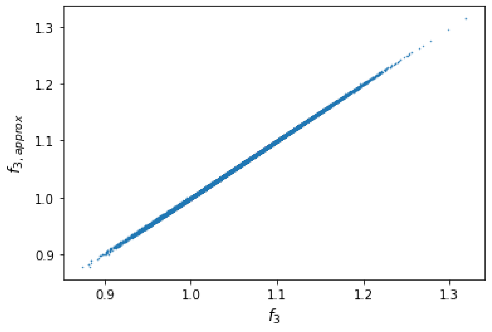
3.1. Results on the Quadratic Approximation of SCR

For the training of our model in Section 2.1 regarding the approximation of the SCR-objective, we have generated 40,000 data points for training and 20,000 points for validation in total. When creating the data set D in (13), we proceeded as follows.
The vectors w l [ 0 , 1 ] 26 describing the investment decision are generated by independently sampling 26 uniformly distributed real numbers in [ 0 , 1 ] with subsequent normalization. With this selection method, we want to avoid strong preferences in investments and thus ensure a high degree of generality. For each w l , we have calculated f 3 ( w l ) , as discussed in Section 1.3 and labeled the outcome as u l = f 3 ( w l ) . This process was repeated 40,000 times to generate training data and 20,000 to generate validation data.
Even if the standard formula is a clear simplification compared to the exact calculation using the loss distribution, it still contains many company-specific variables that can sometimes be difficult to determine. To calculate f 3 ( w l ) , we used a tool which is in operative use in a German insurance company. This tool is part of a decision support software for strategic asset allocation and is used to approximate the effect of an investment decision on the solvency capital on a daily basis. For a detailed description of this tool, we refer to Dächert et al. (2022).
The training of the regression model in Section 2.1 was performed by standard gradient descent using pytorch (Paszke et al. 2019). During the training process over 100 epochs, both the training and validation errors drop quickly and remain at a low level constantly, as indicated in Table 2.
In addition to the mean squared error, we assessed the quality of our approximation via the scatter plot Figure 1.

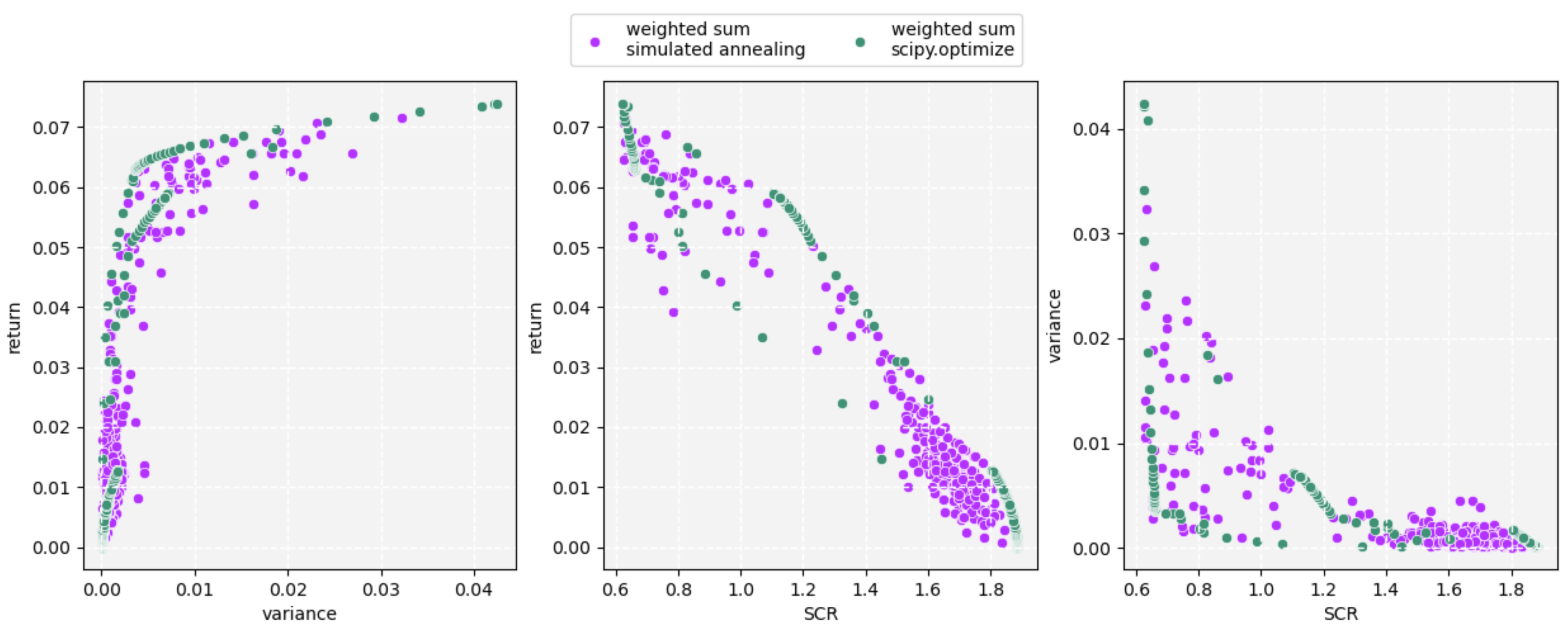
3.2. Results on Solving the Multi-Objective Problem

Since we are interested in obtaining the whole Pareto frontier of the multi-objective problem introduced in (5), we consider various weight vectors for the weighted sum scalarization problem, see (6)–(9). We vary the λ ( λ 1 , λ 2 , λ 3 ) vector using a grid pattern such that λ i { 0 , 0.05 , 0.1 , , 0.95 , 1 } for i = 1 , 2 , 3 and i = 1 3 λ i = 1 . We call that set of weights Λ . Further, we set the factor for the penalty term to λ P = 15 .
We start with a brief assessment of how our chosen discretization of the optimization variables and the penalty term would affect the determination of the Pareto frontier with quantum hardware. Discretization and penalty terms are considered together because they will have a minor impact in the long run and are mainly determined by the hardware limitation (in contrast to the quadratic approximability of the SCR, which is of a fundamental nature). For example, the discretization is determined by the available number of qubits in the quantum hardware.
Figure 2 compares the solutions found for problems (7) and (9). Purple points correspond to (7) and were calculated using SciPy (Virtanen et al. 2020). Green points correspond to (9) and were calculated using D-Wave’s Ocean package for Python, where a simulated annealing algorithm is available, in the form of the function “neal”. The parameters we used for DWave’s neal function were annealingSamples = 200 and annealingTime = 100. Each point (for each color, respectively) is obtained by using a different weight vector λ Λ . The resolution used in the discretization was m = 2 and the penalty factor for the linear equality constrained was λ P = 15 .
The figure shows that, for practical applications, even with a very small resolution of m = 2 , meaningful portfolios can be found on the Pareto frontier. This also shows that even small improvements in the hardware (measured by the qubit number, for example) can be sufficient to enable our method to support decision-making in application-relevant use cases.
Next, we discuss the overall performance of our method by comparing the Pareto frontiers found for (6) and (9). For every λ Λ , we solve (9) via D-Wave’s Ocean package for Python with the same parameters as above. We obtain a list of potential Pareto-optimal solutions. For comparison, we solve (6) for each λ as well using SciPy (Virtanen et al. 2020) as the optimizer. We stress that due to the discretization of the weight vectors λ this is not the whole, continuous Pareto frontier but a very close representation thereof. For the following paragraphs, we assume that the outcome regarding (6) is indeed the Pareto frontier. All calculations have been executed using Python 3.11. The code used in this study is openly available in Braun et al. (2023).
Our main performance index will be the solution quality, answering the question of whether we can find an adequate approximation to the Pareto frontier via our model. For that, we compare the representation of the Pareto frontier computed for (6) with the list of images obtained for (9). We use two different metrics to measure the performance. The first one is a well-known performance measure for multi-objective heuristics, the so-called hypervolume indicator. First introduced to multi-objective optimization by Zitzler and Thiele (1998), it calculates the hypervolume of the area that is dominated by a given set. The area is bounded from (assuming minimization) above by a predefined reference point. For different sets, these hypervolume measurements can be compared. In our experimental study, we use the hypervolume indicator implemented in the pymoo framework Blank and Deb (2020). As a reference point, we use the Nadir point y N a d , defined by y i N a d max x X f i ( x ) , with i { 1 , 2 , 3 } , X R 26 and add a small offset of 0.0001 ; in our case, we calculate the Nadir point for the image under f = ( f 1 , f 2 , f 3 ) of the solutions of (6). The hypervolume indicator is then given as the relative part of the hypervolume that is covered by the images returned by solving (9). A 2D example of the hypervolume and the location of the Nadir point is given in Figure 3.
The second metric stems from the field of approximation. Every solution from the Pareto frontier and every solution obtained by our model has been computed by using a distinct weight vector. For the corresponding weighted sum problem (6), we calculate the approximation factor between this solution and the best one from our QUBO model (9). Overall, we use the worst approximation factor over all weights. Given a weight vector λ = ( λ 1 , λ 2 , λ 3 ) and let x λ be the optimal solution to the corresponding weighted sum problem and X ˜ the set of solutions obtained by our QUBO model, then the approximation factor for this weight vector is given by
A P X ( λ ) min x ˜ X ˜ λ 1 f 1 ( x ˜ ) + λ 2 f 2 ( x ˜ ) + λ 3 f 3 , a p p r o x ( x ˜ ) λ 1 f 1 ( x λ ) + λ 2 f 2 ( x λ ) + λ 3 f 3 ( x λ ) .
The total approximation factor is the maximum over all weight vectors
A P X = max λ Λ A P X ( λ ) .
For the hypervolume indicator we obtain a value of 0.9883, thus less than 2% of the area dominated by the images of the classical solver is not covered by solutions of our model. Thus, this is a very decent result for our heuristic. The approximation factor draws a similar picture: Here, we achieve a total approximation factor A P X of 1.2179. Further, we stress that for 95% of the weight vectors, we obtain an approximation factor of 1.01 or better.
These results show that meaningful portfolios can be generated if, in the portfolio optimization problem, one replaces the SCR according to the standard formula by an appropriately chosen quadratic form. The quadratic form can be found by means of regression, which is a significant reduction in complexity compared to the explicit consideration of the standard formula in the optimization problem. Since it is not to be expected that the quadratic form resulting from the regression is positive-definite and thus convex, the relevance for the practitioner only arises through a combination with an efficient method for non-convex quadratic optimization. For this, quantum computing is a promising candidate. At the time of writing, the quantum hardware is not sufficiently developed to be practically applicable in the insurance industry. As quantum hardware evolves with more qubits and reduced errors, our approach will be a new efficient method to generating relevant portfolios for the practitioner.

4. Conclusions and Future Research

After an overview of classical portfolio theory, we have looked at the importance of Solvency Capital Requirement for insurance companies. It is crucial for insurers to meet their obligations from old policies (with high guaranteed interest rates) and at the same time fulfill the regulatory requirements for their risk profile. It is, therefore, important to extend the traditional Markowitz model to include the SCR alongside the usual objectives of expected return and volatility. However, it should be noted that considering the SCR in an optimization problem usually involves a considerable amount of time and computational effort.
For this, we have approximately translated the SCR calculation (according to the standard formula) into a quadratic form, thus making it accessible to methods for solving QUBOs. Since return and volatility can be written as QUBOs from the outset, it is possible to perform the entire portfolio optimization problem (including SCR) on the quantum computer. As soon as high-performing annealing hardware or Quantum Computers are available, this formulation can be used to solve the portfolio optimization with SCR, possibly with a meaningful speed advantage over classical solutions.
The quadratic form for the SCR standard formula was found by means of a machine learning algorithm. The idea of using a machine learning algorithm to build an approximate QUBO might be applied successfully in different contexts and might be considered the main contribution of this work.
Of interest for future research is the consideration of further economically relevant objective functions, such as key figures from the IFRS balance sheet or valuation reserves. Moreover, expanding the focus beyond QUBOs, for example, by allowing higher degree polynomials for approximation, could provide further interesting applications for quantum computing.

Author Contributions

All authors contributed to all aspects of this work. All authors have read and agreed to the published version of the manuscript.

Funding

This research was funded by Bundesministerium für Bildung und Forschung (BMBF), grant number 13N15695.

Data Availability Statement

The data presented in this study are available on request from the corresponding author. The data are not publicly available due to privacy.

Conflicts of Interest

Author Mohammad Assadsolimani was employed by the company DZ BANK AG. Author Janik Maciejewski was employed by the company R+V Lebensversicherung AG. Authors Markus Braun, Niklas Hegemann and Sven Kerstan were employed by the company JoS QUANTUM GmbH. The authors declare that the research was conducted in the absence of any commercial or financial relationships that could be construed as a potential conflicts of interest.

Appendix A

The following table contains the correlation coefficients for the 26 asset classes from our use case in Section 3. Assets appear in the same order as in Table 1.
1.0 0.7 0.1 0.2 0.2 0.1 0.2 0.1 0.0 0.1 0.1 0.1 0.1 0.2 0.2 0.1 0.2 0.1 0.2 0.3 0.1 0.2 0.1 0.0 0.0 0.0 0.7 1.0 0.1 0.2 0.2 0.1 0.1 0.0 0.0 0.0 0.0 0.1 0.2 0.2 0.2 0.2 0.2 0.1 0.2 0.2 0.1 0.1 0.1 0.0 0.0 0.0 0.1 0.1 1.0 0.1 0.1 0.5 0.6 0.8 0.7 0.7 0.7 0.6 0.1 0.4 0.4 0.1 0.2 0.3 0.2 0.3 0.6 0.6 0.5 0.6 0.0 0.0 0.2 0.2 0.1 1.0 0.9 0.3 0.2 0.1 0.2 0.1 0.1 0.0 0.8 0.7 0.7 0.8 0.8 0.4 0.9 0.8 0.0 0.0 0.6 0.3 0.0 0.0 0.2 0.2 0.1 0.9 1.0 0.4 0.2 0.1 0.1 0.1 0.1 0.0 0.9 0.6 0.7 0.8 0.8 0.4 0.9 0.7 0.0 0.0 0.7 0.3 0.0 0.0 0.1 0.1 0.5 0.3 0.4 1.0 1.0 0.5 0.3 0.5 0.5 0.4 0.3 0.5 0.7 0.4 0.4 0.8 0.4 0.5 0.8 0.6 0.7 0.5 0.0 0.0 0.2 0.1 0.6 0.2 0.2 1.0 1.0 0.5 0.4 0.6 0.5 0.4 0.1 0.4 0.6 0.3 0.4 0.7 0.2 0.4 0.9 0.7 0.7 0.5 0.0 0.0 0.1 0.0 0.8 0.1 0.1 0.5 0.5 1.0 0.9 0.9 0.8 0.8 0.1 0.3 0.3 0.1 0.1 0.2 0.0 0.1 0.6 0.7 0.3 0.5 0.0 0.0 0.0 0.0 0.7 0.2 0.1 0.3 0.4 0.9 1.0 0.8 0.7 0.7 0.2 0.3 0.2 0.2 0.0 0.0 0.1 0.1 0.5 0.7 0.2 0.4 0.0 0.0 0.1 0.0 0.7 0.1 0.1 0.5 0.6 0.9 0.8 1.0 0.8 0.7 0.2 0.3 0.3 0.2 0.1 0.2 0.0 0.1 0.7 0.8 0.3 0.4 0.0 0.0 0.1 0.0 0.7 0.1 0.1 0.5 0.5 0.8 0.7 0.8 1.0 0.6 0.1 0.3 0.4 0.1 0.1 0.2 0.0 0.2 0.6 0.7 0.3 0.6 0.0 0.0 0.1 0.1 0.6 0.0 0.0 0.4 0.4 0.8 0.7 0.7 0.6 1.0 0.1 0.4 0.3 0.1 0.1 0.2 0.0 0.2 0.5 0.6 0.3 0.4 0.0 0.0 0.1 0.2 0.1 0.8 0.9 0.3 0.1 0.1 0.2 0.2 0.1 0.1 1.0 0.6 0.7 0.8 0.7 0.3 0.8 0.6 0.1 0.0 0.6 0.3 0.0 0.0 0.2 0.2 0.4 0.7 0.6 0.5 0.4 0.3 0.3 0.3 0.3 0.4 0.6 1.0 0.8 0.5 0.7 0.4 0.8 0.8 0.3 0.5 0.6 0.4 0.0 0.0 0.2 0.2 0.4 0.7 0.7 0.7 0.6 0.3 0.2 0.3 0.4 0.3 0.7 0.8 1.0 0.6 0.8 0.5 0.7 0.9 0.4 0.6 0.7 0.5 0.0 0.0 0.1 0.2 0.1 0.8 0.8 0.4 0.3 0.1 0.2 0.2 0.1 0.1 0.8 0.5 0.6 1.0 0.7 0.7 0.7 0.6 0.1 0.1 0.8 0.3 0.0 0.0 0.2 0.2 0.2 0.8 0.8 0.4 0.4 0.1 0.0 0.1 0.1 0.1 0.7 0.7 0.8 0.7 1.0 0.4 0.8 0.7 0.2 0.3 0.7 0.3 0.0 0.0 0.1 0.1 0.3 0.4 0.4 0.8 0.7 0.2 0.0 0.2 0.2 0.2 0.3 0.4 0.5 0.7 0.4 1.0 0.3 0.4 0.6 0.2 0.7 0.4 0.0 0.0 0.2 0.2 0.2 0.9 0.9 0.4 0.2 0.0 0.1 0.0 0.0 0.0 0.8 0.8 0.7 0.7 0.8 0.3 1.0 0.7 0.0 0.2 0.6 0.3 0.0 0.0 0.3 0.2 0.3 0.8 0.7 0.5 0.4 0.1 0.1 0.1 0.2 0.2 0.6 0.8 0.9 0.6 0.7 0.4 0.7 1.0 0.3 0.3 0.6 0.4 0.0 0.0 0.1 0.1 0.6 0.0 0.0 0.8 0.9 0.6 0.5 0.7 0.6 0.5 0.1 0.3 0.4 0.1 0.2 0.6 0.0 0.3 1.0 0.7 0.5 0.5 0.0 0.0 0.2 0.1 0.6 0.0 0.0 0.6 0.7 0.7 0.7 0.8 0.7 0.6 0.0 0.5 0.6 0.1 0.3 0.2 0.2 0.3 0.7 1.0 0.4 0.5 0.0 0.0 0.1 0.1 0.5 0.6 0.7 0.7 0.7 0.3 0.2 0.3 0.3 0.3 0.6 0.6 0.7 0.8 0.7 0.7 0.6 0.6 0.5 0.4 1.0 0.6 0.0 0.0 0.0 0.0 0.6 0.3 0.3 0.5 0.5 0.5 0.4 0.4 0.6 0.4 0.3 0.4 0.5 0.3 0.3 0.4 0.3 0.4 0.5 0.5 0.6 1.0 0.0 0.0 0.0 0.0 0.0 0.0 0.0 0.0 0.0 0.0 0.0 0.0 0.0 0.0 0.0 0.0 0.0 0.0 0.0 0.0 0.0 0.0 0.0 0.0 0.0 0.0 1.0 0.0 0.0 0.0 0.0 0.0 0.0 0.0 0.0 0.0 0.0 0.0 0.0 0.0 0.0 0.0 0.0 0.0 0.0 0.0 0.0 0.0 0.0 0.0 0.0 0.0 0.0 1.0

References

  1. Artzner, Philippe, Freddy Delbaen, Eber Jean-Marc, and David Heath. 1999. Coherent measures of risk. Mathematical Finance 9: 203–28. [Google Scholar] [CrossRef]
  2. Bauer, Daniel, Andreas Reuss, and Daniela Singer. 2012. On the calculation of the solvency capital requirement based on nested simulations. ASTIN Bulletin 42: 453–99. [Google Scholar] [CrossRef]
  3. Blank, Julian, and Kalyanmoy Deb. 2020. pymoo: Multi-objective optimization in python. IEEE Access 8: 89497–509. [Google Scholar] [CrossRef]
  4. Braun, Markus, Thomas Decker, Marcelin Gallezot, Niklas Hegemann, Sven Kerstan, and Yuanheng Zhou. 2023. pygrnd. Available online: https://github.com/JoSQUANTUM/pygrnd (accessed on 29 November 2023).
  5. Dächert, Kerstin, Ria Grindel, Elisabeth Leoff, Jonas Mahnkopp, Florian Schirra, and Jörg Wenzel. 2022. Multicriteria asset allocation in practice. OR Spectrum 44: 349–73. [Google Scholar] [CrossRef]
  6. Ehrgott, Matthias. 2005. Multicriteria Optimization. Berlin: Springer Science & Business Media, vol. 491. [Google Scholar]
  7. Elsokkary, Nada, Faisal Shah Khan, Davide La Torre, Travis S. Humble, and Joel Gottlieb. 2017. Financial portfolio management using adiabatic quantum optimization: The case of abu dhabi securities exchange. Paper presented at 2017 IEEE High Performance Extreme Computing Conference (HPEC), Waltham, MA, USA, September 12–14; pp. 1–4. [Google Scholar]
  8. European Commission. 2015. Commission Delegated Regulation (eu) 2015/35. Available online: https://eur-lex.europa.eu/legal-content/EN/TXT/PDF/?uri=CELEX:32015R0035&rid=1 (accessed on 29 November 2023).
  9. European Parliament and European Council. 2009. Directive 2009/138/ec. Available online: https://eur-lex.europa.eu/LexUriServ/LexUriServ.do?uri=OJ:L:2009:335:0001:0155:en:PDF (accessed on 29 November 2023).
  10. Halffmann, Pascal, Luca E. Schäfer, Kerstin Dächert, Kathrin Klamroth, and Stefan Ruzika. 2022. Exact algorithms for multiobjective linear optimization problems with integer variables: A state of the art survey. Journal of Multi-Criteria Decision Analysis 29: 341–63. [Google Scholar] [CrossRef]
  11. IBM. 2023. Available online: https://newsroom.ibm.com/2023-12-04-IBM-Debuts-Next-Generation-Quantum-Processor-IBM-Quantum-System-Two,-Extends-Roadmap-to-Advance-Era-of-Quantum-Utility (accessed on 25 January 2024).
  12. Jonen, Christian, Tamino Meyhöfer, and Zoran Nikolić. 2023. Neural networks meet least squares monte carlo at internal model data. European Actuarial Journal 13: 399–425. [Google Scholar] [CrossRef]
  13. Krah, Anne-Sophie, Zoran Nikolić, and Ralf Korn. 2020. Least-squares monte carlo for proxy modeling in life insurance: Neural networks. Risks 8: 116. [Google Scholar] [CrossRef]
  14. Markowitz, Harry. 1952. Portfolio Selection. Journal of Finance 7: 77–91. [Google Scholar] [CrossRef]
  15. Nelder, John Ashworth, and Robert W. M. Wedderburn. 1972. Generalized linear models. Journal of the Royal Statistical Society Series A: Statistics in Society 135: 370–84. [Google Scholar] [CrossRef]
  16. Paszke, Adam, Sam Gross, Francisco Massa, Adam Lerer, James Bradbury, Gregory Chanan, Trevor Killeen, Zeming Lin, Natalia Gimelshein, Luca Antiga, and et al. 2019. Pytorch: An imperative style, high-performance deep learning library. In Advances in Neural Information Processing Systems 32. Red Hook: Curran Associates, Inc., pp. 8024–35. [Google Scholar]
  17. Rosenberg, Gili, Poya Haghnegahdar, Phil Goddard, Peter Carr, Kesheng Wu, and Marcos López De Prado. 2015. Solving the optimal trading trajectory problem using a quantum annealer. Paper presented at 8th Workshop on High Performance Computational Finance, Austin, TX, USA, November 15; pp. 1–7. [Google Scholar]
  18. Seelbach Benkner, Marcel, Maximilian Krahn, Edith Tretschk, Zorah Lähner, Michael Moeller, and Vladislav Golyanik. 2023. QuAnt: Quantum Annealing with Learnt Couplings. Paper presented at International Conference on Learning Representations (ICLR), Kigali, Rwanda, May 1–5. [Google Scholar]
  19. Shalev-Shwartz, Shai, and Shai Ben-David. 2014. Understanding Machine Learning. Cambridge: Cambridge University Press. [Google Scholar]
  20. Somma, Rolando D., Daniel Nagaj, and Mária Kieferová. 2012. Quantum speedup by quantum annealing. Physical Review Letters 109: 050501. [Google Scholar] [CrossRef] [PubMed]
  21. Venturelli, Davide, and Alexei Kondratyev. 2019. Reverse quantum annealing approach to portfolio optimization problems. Quantum Machine Intelligence 1: 17–30. [Google Scholar] [CrossRef]
  22. Virtanen, Pauli, Ralf Gommers, Travis E. Oliphant, Matt Haberland, Tyler Reddy, David Cournapeau, Evgeni Burovski, Pearu Peterson, Warren Weckesser, Jonathan Bright, and et al. 2020. SciPy 1.0: Fundamental Algorithms for Scientific Computing in Python. Nature Methods 17: 261–72. [Google Scholar] [CrossRef] [PubMed]
  23. Zhou, Leo, Sheng-Tao Wang, Soonwon Choi, Hannes Pichler, and Mikhail D Lukin. 2020. Quantum approximate optimization algorithm: Performance, mechanism, and implementation on near-term devices. Physical Review X 10: 021067. [Google Scholar] [CrossRef]
  24. Zitzler, Eckart, and Lothar Thiele. 1998. Multiobjective optimization using evolutionary algorithms—A comparative case study. In Parallel Problem Solving from Nature—PPSN V. Edited by Agoston E. Eiben, Thomas Bäck, Marc Schoenauer and Hans-Paul Schwefel. Berlin/Heidelberg: Springer, pp. 292–301. [Google Scholar]
Figure 1. Scatter plot with values of f 3 ( w l ) and f 3 , a p p r o x ( w l ) for every sampled portfolio vector w l from the validation data.
Risks 12 00023 g001
Figure 2. Pareto frontiers for the portfolio optimization problem according to Equation (7) in purple and according to Equation (9) in green. Both use the n = 26 asset classes with their returns and the covariance matrix we described in Table 1. The QUBO solutions were generated with a resolution of m = 2 bits. A penalty factor of P = 15 was used to enforce the constraint that all funds are invested. The different points each correspond to a single solution using a weighted sum, each with different weights. This illustrates that the QUBO formulation can indeed give very similar solutions to the standard, continuous formulation with the constraint (that the available capital must be fully invested in the available asset classes), even for low resolutions.
Risks 12 00023 g002
Figure 3. A 2D example of the hypervolume indicator. The blue area is the area dominated by the Pareto frontier and is spanned by the images in the Pareto frontier (blue points) and the reference point y r e f . The reference point is computed by the Nadir point plus a small offset. The red points are the objective function values of the solutions obtained by the heuristic and the red area is the corresponding dominated area. In this example, the hypervolume indicator, calculated by counting the covered tiles, is 16.67%.
Risks 12 00023 g003
Table 1. Asset classes that we consider in our use case. The column μ i contains the expected return and σ i , i the variance, both given in percent. The correlations are given in the Appendix A.
Asset Class i μ i σ i , i Asset Class i μ i σ i , i
1 3 ,   4 2 ,   8 14 1 ,   3 3 ,   4
2 6 ,   0 9 ,   2 15 1 ,   5 3 ,   8
3 6 ,   5 12 ,   6 16 3 ,   0 4 ,   7
4 1 ,   9 1 ,   9 17 1 ,   6 3 ,   6
5 1 ,   3 4 ,   2 18 3 ,   7 9 ,   3
6 5 ,   6 7 ,   0 19 0 ,   2 2 ,   5
7 6 ,   4 8 ,   7 20 1 ,   1 1 ,   3
8 4 ,   0 13 ,   5 21 5 ,   8 8 ,   3
9 6 ,   5 17 ,   8 22 3 ,   5 9 ,   4
10 6 ,   5 18 ,   4 23 2 ,   4 6 ,   9
11 6 ,   7 17 ,   4 24 1 ,   2 9 ,   3
12 7 ,   4 20 ,   6 25 3 ,   0 8 ,   0
13 0 ,   9 3 ,   9 26 0 ,   0 1 ,   0
Table 2. The development of training and validation errors during 100 epochs. After only a few epochs, the algorithm finds an approximation with sufficient accuracy. The low validation error suggests good generalizability without overfitting.
Epoch1210100
Training Error 3 × 10 1 4 × 10 4 1 × 10 5 4 × 10 7
Validation Error 9 × 10 1 7 × 10 2 5 × 10 4 5 × 10 7
Disclaimer/Publisher’s Note: The statements, opinions and data contained in all publications are solely those of the individual author(s) and contributor(s) and not of MDPI and/or the editor(s). MDPI and/or the editor(s) disclaim responsibility for any injury to people or property resulting from any ideas, methods, instructions or products referred to in the content.

