1. Introduction
Research on innovative and strategic retirement financing approaches is increasingly compelling and imperative as aging populations become national and social issues for most countries. As more pension plans have shifted from defined benefit (DB) to defined contribution (DC), most pensioners gradually realize that they have not contributed enough to maintain their expected living standards in retirement, and they are eager to explore alternative retirement financing approaches. The obvious and simple alternative is to find a way to release their property value without selling it, if possible.
For many asset-rich-cash-poor homeowners, most of their accumulated wealth is usually tied up in their property. When they reach the stage of planning and preparing for their retirement, they face the challenge of converting part of their property into regular retirement income if they want to stay in their property for life. Equity release products are a viable and popular solution for this cohort of people to unlock the value of their properties without selling or renting out the properties. These financial instruments, which were first transacted in 1961 through Deering Saving & Loan in the US, have been gaining popularity over the years in many countries as an option for retirees to fund their retirement and improve their quality of life. Two well-known equity release products, a loan-type Reverse Mortgage (RM) plan and a sell-type Home Reversion (HR) plan, entitle homeowners to live in their properties for life and convert the assets into streams of stable income for retirement. As existing equity release plans are relatively complex and opaque, most consumers may not be able to understand their costs and benefits or to make meaningful comparisons. As a result, equity release markets are relatively small and underdeveloped in most countries.
By joining an RM plan, a homeowner incurs a loan from a bank and receives cash payouts according to their needs and financial objectives in various ways, including an upfront cash payout, monthly installments, a line of credit, or a combination of these options. During the term of the loan, the homeowner is entitled to live on the property without obligations to make any repayments as interest on the loan accrues over time with an increasing loan balance. However, as the loan balance grows exponentially with accumulated interest, it will substantially reduce the equity value left in the property to be inherited. The loan balance is typically repaid when the homeowner sells the house, moves out, or passes away. After the property is sold, if the sale proceeds from the property are more than the outstanding loan balance, the surplus is returned to the homeowner or their inheritance. On the other hand, any shortfall in the proceeds for repaying the loan is borne by an insurance arrangement as RM is a non-recourse loan. The pricing and hedging of non-recourse loan risk has been extensively studied by
Chen et al. (
2010),
Li et al. (
2010),
Lee et al. (
2012),
Kogure et al. (
2014),
Shao et al. (
2015), and
Wang et al. (
2016), to name a few. Despite most retirees appearing to be unaware of or unfamiliar with RM, this loan type has been developed to become the most popular and widely-available equity release product in many countries, such as the US (
Shan 2011), UK (
Sharma et al. 2022), Australia (
Ong 2009), Korea (
Kim and Li 2016), Japan (
Mitchell and Piggott 2004), Spain (
Debon et al. 2013), etc. In addition to using RM as a source of financial income,
Stucki (
2006),
Andrews and Oberoi (
2015), and
Bonnet et al. (
2019) also explored the opportunities and challenges in linking RM with long-term care (LTC) needs and financing.
HR plans, which are a less common and popular form of equity release product compared with RM, are only available in some countries, such as Australia and the UK. Under HR plans, a homeowner sells a portion of the home value to obtain an upfront payment, regular payments, or a combination of both while retaining the property title and the right to age in place. In other words, the homeowner shares a contractual portion of the future property sale proceeds with the product provider in exchange for receiving immediate financial benefits and the right to live in the property without paying any rent until death. When the property is sold, typically after the death of the homeowner, the sale proceeds are divided according to the ownership percentages of the homeowner and product provider. Since HR is a sell-type product that does not accrue any loan interest, the amount left for inheritance is equivalent to the portion of the unsold property and is more valuable for homeowners who want to provide a bequest to their estates, compared with RM. Even though the discussion of HR plans is surprisingly sparse in the actuarial literature,
Alai et al. (
2014) provide an extensive risk comparison between RM and HR in terms of value-at-risk and conditional value-at-risk measures.
Hanewald et al. (
2015) investigated the timing decision of when to optimally release equity through RM and HR, while
Xiao (
2011) explored and discussed a contract linking HR and LTC needs.
By contrast, a less well-known Lease Buyback Scheme (LBS)—a unique equity release plan only available in Singapore—provides an alternative sell-type equity release product for public properties with minimum cashflow uncertainty. In particular, LBS provides a predetermined period for the owner to stay on the property without incurring any insurance costs or loan costs by giving up the future value of the whole property, as there is no non-recourse guarantee or aging-in-place guarantee. Therefore, stochastic house prices, interest rates, and mortality risks do not need to be considered in the pricing model. As a result, LBS does not provide the homeowner any right to live in the property for life and any entitlement to benefit from the possibility of property appreciation.
Kwong et al. (
2021) discussed the pricing LBS model to assess the costs and benefits of the product.
The other sell-type hybrid equity release (HER) plan proposed by
Kwong et al. (
2021) incorporates features of both the HR and the LBS, with an actuarial framework to analyze the pricing of the HER. Under HER, a homeowner sells a portion of the property to a plan provider at a discounted price, similar to the HR transaction. In contrast, the homeowner is given a right to stay in the property for a certain period without depending on survival, similar to the LBS transaction. Should the owner survive after that period, they can still stay on the property until death. In conclusion, HER provides a predetermined period for the owner and their family to stay in the property, as well as a guarantee of aging-in-place after that period.
When comparing the product benefits given by both types of equity release plans from the homeowner’s perspective, most homeowners should prefer the sell-type plan to the loan-type plan as the former involves no interest rate risk, shifts part of property price risk to plan providers, and provides a fixed proportion of property value as bequests. However, the real-life situation shows that the loan-type RM plan either dominates equity release market share in most countries or is the only available product for homeowners as most plan providers controlling the supply of equity release plans prefer to offer RM to suit their risk portfolio management and the weak homeowners’ demand has little or no influence on the development of sell-type equity release market. We will highlight the issue of weak demand for current sell-type plans and explore some possible ways of addressing the issue. By designing more new product features of sell-type plans to meet a broader spectrum of homeowners’ financial needs, we expect that the possible, increasing demand for new sell-type products may stimulate more sell-type product supply and then change the landscape of equity release markets.
In this study, we propose a new sell-type equity release product called Enhanced Home Reversion (EHR), which has new features to meet homeowners’ specific needs beyond providing a guaranteed period to stay in the property. In the next section, we provide background knowledge of current sell-type equity release products. Then, we outline the new features of the proposed EHR plan and discuss an actuarial approach for evaluating their actuarial values in
Section 3. With the actuarial models for new product features, we focus on the numerical discussion of cost–benefit and risk analysis of the product features and compare EHR with other sell-types products under the Singapore mortality data set in
Section 4. A conclusion is given in
Section 5.
2. Reviews of Sell-Type Equity Release Products
Compared with loan-type equity release products, sell-type equity release products have three major advantages from the homeowner’s perspective: they are not subject to any interest rate risk, they keep a certain portion of the property value as a bequest, and they shift a proportion of property price risk to the plan provider. In this study, therefore, we focus on the discussion of developing more features of sell-type equity release products to meet other financial and retirement needs.
2.1. Home Reversion Plan
Under the sell-type Home Reversion (HR) plan, the homeowner sells a predetermined proportion of the property value to a plan provider at a discounted price () according to their financial needs, where is the current property market value. By selling the property proportion at a discounted price, the owner retains the home title and the right to live in the property until the death or sale of the property. In other words, the homeowner gives up a contractual proportion of the future home sale proceeds (, where is the price of property sold at time ) in exchange for receiving an immediate lump-sum payment and the right to age in place. The parameter value depends on the homeowner’s mortality rate and the rental cost. The higher mortality rate and lower rental cost imply a larger value as the expected actuarial cost of staying for life is lower. As the HR plan is not a loan-type product, not only does it face no interest rate risk, but the amount of bequest can also be fixed at the future sale remaining proceeds (). Although the homeowner enjoys the certainty of a bequest feature that cannot be found in any loan-type equity release products, they are subjected to the risk of financial loss in case of an earlier-than-expected death. This significant financial loss risk may be one of the major reasons why HR is not widely available and less popular when compared with loan-type products.
2.2. Singapore Lease Buyback Scheme
The Housing & Development Board (HDB), established in 1960, is the delegated public housing authority that develops quality and affordable flats for residents (citizens or permanent residents) in Singapore. In 2023, more than 1 million HDB flats housed 80% of Singapore residents, of which about 90% own their own flats. In general, all new HDB flats are directly sold to qualifying residents under 99-year leasehold agreements by the HDB.
Lease Buyback Scheme (LBS), the only available equity release product in Singapore and introduced by the HDB in 2009 to help flat owners release their flat values, divides a flat’s remaining lease period into a front-end lease and a tail-end lease. Under LBS, HDB flat owners have the right to stay in the flat until the front-end lease expires while the flat’s tail-end lease is sold back to HDB for retirement funding. For example, if the flat’s current remaining lease is 65 years and the flat owner sells the 35-year tail-end lease to HDB, the owner can then stay in the flat for the next 30 years under the front-end lease without paying any rent.
1 The amount of initial cashflow to flat owners is equivalent to the present value of the tail-end lease sold, which can be determined as the difference between the flat’s market value and the present value of the front-end lease with the necessary adjustments due to the restrictive conditions and terms imposed on the flat owner.
If necessary, the owner may release the entire value of the flat by selling the flat back to the HDB during the front-end lease period in return for a refund on the remaining front-end lease period, pro-rata on a straight-line basis. If the flat owner dies before the expiry of the front-end lease, immediate family members living in the flat are allowed to either stay for the rest of the front-end lease balance or return the flat to the HDB with a pro-rata refund. However, the flat owner is required to move out of the flat and return it to the HDB at the expiry of the front-end lease. Therefore, the LBS does not provide the owner any guarantee of living in the flat for life or any financial benefits due to future flat value appreciation. As a result, LBS should be considered a deterministic financial product that is not subject to any risks on the stochastic flat value, interest rate, and mortality rate, according to
Kwong et al. (
2021).
2.3. Hybrid Equity Release Plan
Similar to the HR plan, the other sell-type Hybrid Equity Release (HER) plan provides homeowners with a right to stay for life or a fixed period, whichever is longer, by selling a proportion of flat value to the plan provider at a price . Specifically, the homeowner chooses a length of period years of staying in the property irrespective of their survival. In the event the owner survives after years, they are entitled to stay in the property until death. Thus, is the minimum period the owner and their family have the right to stay. Upon the death of the owner after years, the property will be sold, and the owner’s beneficiaries will receive portion of the sale proceeds. In conclusion, HER provides the owner not only with the right to stay in the property for life or a fixed period, whichever is longer, but the estate can also retain a fixed proportion of the sale proceeds and realize the potential asset appreciation. If a large under HER is chosen, it implies that the owner pays a relatively low cost for this deferred insurance of staying in the property until death and faces a more predictable financial outcome. Property owners who do not need to have a long guaranteed period of staying in the property may choose a small value of . With smaller under HER, the owner pays a higher insurance cost of aging-in-place which implies facing a higher risk of financial loss if the owner dies too early.
3. Enhanced Home Reversion Plan
By considering homeowners’ other financial needs, we now propose and outline a new sell-type equity release product, called the Enhanced Home Reversion (EHR) plan, with new product features to meet a larger group of homeowners’ needs. Consider a homeowner aged () joining the new plan. For easy illustration, we present the time unit in months instead of years in this study. Let be the discount factor for one month corresponding to the monthly interest rate , so that . The monthly interest rate may be considered as the underlying deterministic constant interest rate assumption. We may estimate the monthly interest rate based on the current yield of insurance products in the market.
Denote
as the curtate future lifetime of (
) in the number of complete months for
. Let
for
and 0 otherwise be the present value of death benefit random variable for
-month term life insurance of
, payable at the time of end of month
. Similarly, the present value of the benefit random variable for a whole life annuity due of 1 per month, payable monthly while (
) survives, is
for
= 0, 1, …, where
, effective discount rate per month.
2 Thus, the expected values of
and
are
and
, respectively.
3.1. Life Annuity and Decreasing Term Life Insurance Features
Under HR and HER, the initial amount of cash payout may exceed the needs of the homeowner and does not necessarily provide a reliable stream of stable income for retirement. The EHR plan adds the first new feature of life annuity payments, which are payable upon the homeowner’s survival. However, similar to HR and HER, the EHR life annuity and aging-in-place guarantee features expose the homeowner to a large risk of financial disadvantage if the homeowner dies too early after signing up for the plan. In addition,
Blake (
1999) highlighted the problems of providing life annuity products, such as interest rate risk, adverse selection, and mortality improvement, to name a few.
To hedge the financial risk faced by the plan provider and homeowner, the EHR plan’s second new feature introduces monthly decreasing term life insurance incorporated into the product. The amount of death benefit under term insurance will be reduced each month by the amount of the monthly annuity payment and the implied monthly rental value payable to the plan provider. With this product feature, the shorter the period the homeowner can live in the house, the greater the amount of death benefit that will be payable. As a result, the financial loss of the unexpected early death of the homeowner is strategically hedged under these two new features. In essence, the EHR plan provides a guarantee of returning the principal amount invested to the homeowner and reduces the provider’s product risk. In fact, for some countries where gender pricing is not allowed, these two new features effectively reduce the financial impact of no-gender pricing restriction as the total cost of product features is not too sensitive to the mortality rate.
The new EHR plan is designed in such a way that the amount of partial property sold is used to pay for four benefits: the upfront cash payout to the homeowner, the cost of a life annuity, the cost of staying in the property for life, and the cost of monthly-decreasing term life insurance. From the homeowner’s perspective, the present value of the future loss random variable in the scheme issued to (
) is
where
is the monthly rental amount,
is the amount of each annuity payment to the homeowner per month, and
is the monthly-decreasing term insurance that matures in
months and can be determined by the ratio
rounded down to the nearest integer. Note that the numerator of the ratio
is the invested principal amount being equal to the difference between the amount of property sold and the amount of upfront payment, while the denominator is the amount of survival benefits that the owner enjoys in each month. Therefore, the ratio
implies the maximum number of months the invested principal amount can cover the survival benefits. If the homeowner can survive up to the expiration of term insurance, the invested principal amount is returned to the owner as survival benefits. On the other hand, if the homeowner dies
months later, the death benefit from term insurance (
plus the survival benefit (
enjoyed by the owner are still equivalent to the invested principal amount.
3.2. Costs of New Features
After taking the expectation on both sides of (1), we apply the actuarial equivalence principle with the actuarial present value of cash inflows equal to the actuarial present value of cash outflows, or
, and obtain
According to (2), the sold property value covers the costs of four benefits offered to the homeowner under the plan. The first benefit is the amount of upfront payment to the owner. The second benefit is the right of aging-in-place. The third benefit is the cost of life annuity payable to the homeowner. The fourth benefit is the actuarial present value of -month decreasing term insurance.
3.3. Hedging of New Features
By considering the random components of (1), we modify the present value of the benefits variable
from the new features as follows:
Note that the benefit variable W is a positive decreasing function of for , and becomes a positive increasing function of for (after the term insurance expires). Therefore, the minimum value of W is at and it implies that the hedging effect of product features reduces the impact of financial loss due to premature death.
4. Numerical Analysis of New Product’s Features
The new EHR features not only provide an option of keeping a portion of property value as a bequest but also have a possible death benefit as an additional bequest for early unexpected death. Upon a homeowner’s death
complete months after joining the plan and selling the property at the price
, the amount of bequest,
is determined as follows:
As time goes on, the owner enjoys more benefits of staying in their home and annuity payments. The amount of bequest from the death benefit of term insurance decreases gradually until the maturity of
-month term insurance. With the extra term insurance cost
, the death benefit from term insurance acts as a tool for providing a guaranteed return of principal amount for the homeowner in the worst-case scenarios, according to the discussion in
Section 3.3.
4.1. Cost Analysis
With the new EHR features, the homeowner needs to make two key decisions according to personal preferences when buying the product. First, the owner determines the proportion of the future home value proceeds to be sold. Second, the owner chooses the proportion of home value to be payable upfront. The first parameter controls the potential amount of bequest as the larger implies the smaller bequest amount . The second parameter determines the monthly amount of annuity payable since the larger leads to a smaller amount of monthly payment . In general, choosing the maximum value of for a chosen , implies no benefits of annuity payments and term insurance coverage, and EHR reduces to a typical Home Reversion (HR) product.
For a typical HR product with only benefits
and
offered to the owners if the owner chooses
with calculated
aging-in-place cost component for a given combination of age and gender, then the maximum value
, denoted as
, can be determined by
. Therefore, the second parameter must be chosen within the upper bound
or
for the new features of EHR and at
for HR. Denote
, the amount of cash upfront under an HR product with
. Similarly, for the Hybrid Equity Release (HER) plan, we define the aging-in-place cost component with a guaranteed fixed period
s of staying as
and the proportion of cash upfront cash payout can be determined as
. The evaluations of
and
for given
s can be referred to
Kwong et al. (
2021) for details.
For illustrative purposes, consider a hypothetical example of selling the equity release products to a homeowner with a
$1 million house with an estimated
monthly rent (about
annual rental yield rate) and
per month with mortality assumption following the Singapore 2022 Preliminary Life Tables (
Singapore Department of Statistics 2023)
3. We now examine the cost components with respect to different combinations of product options:
,
and demographic factors: gender, and age under three different sell-type products discussed here.
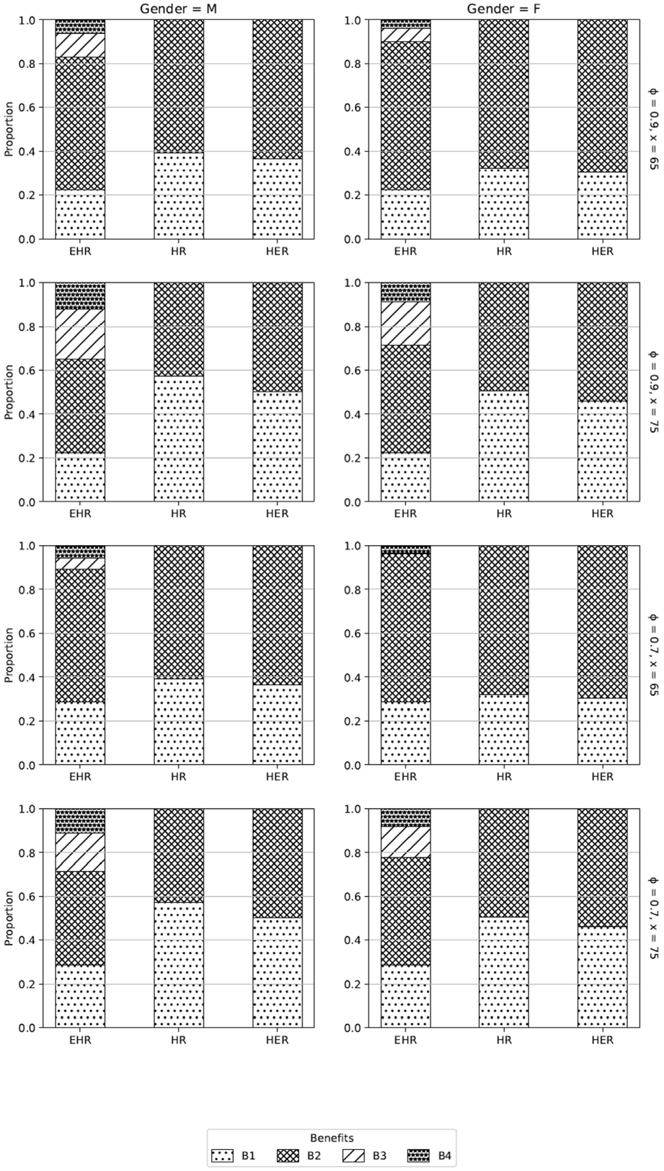
Figure 1 summarizes the results of the cost proportions with different combinations of configurations:
,
under EHR,
under HR,
with
under HER,
for male and female owners. As observed in
Figure 1, the cost proportion of initial cash outflow
for HER with
is consistently less than HR’s
. This is expected as this HER provides the owner the extra benefit of staying in the property for 10 years without depending on survival. In return for this extra benefit, the owner under HER receives a lower cash payment proportion
. As EHR covers the additional cost components of life annuity (
) and decreasing term insurance (
) without any fixed period of staying in the property, the
and
proportions under EHR are consistently less than the
and
proportions under HER with
. For example, for males with
,
, we observe that proportions
,
are (0.22, 0.61) for EHR and (0.36, 0.64) for HER with
.
Note that proportions regardless of the values of and are the same for EHR and HR as both have the same cost of aging-in-place for a given demographic factor. In addition, the proportion decreases as participating age increases for both genders and all products. For example, for males with , we observe that proportion of EHR decreases from 0.61 at age 65 to 0.43 at age 75. Similarly, for females with , we observe that proportion decreases from 0.68 at age 65 to 0.49 at age 75. At the same time, our results consistently demonstrate that females need to pay a slightly higher proportion of at any age level. This is in line with the notion that as females have a lower mortality rate than males, their cost proportion of aging-in-place will correspondingly be higher for all the products considered here.
Finally, the cost proportions and under EHR increase as the participating age increases. This is because term insurance is more expensive for older owners than younger owners, and the amount of life annuity payments is significantly higher for older owners than for younger owners under EHR. For example, with , we observe the proportion almost doubles from 6.2% for males aged 65 to 12.1% for males aged 75, and the proportion increases from 11.0% for males aged 65 to 23.0% for males aged 75, where the monthly annuity payments are $685 and $2031 for males aged 65 and 75, respectively. Note that if the bequest amount is not a key concern for the owners, older owners may consider removing the term insurance components to increase the number of annuity payments or to give up the principal return guarantee benefit.
4.2. Risk Analysis
The EHR plan strategically includes the death benefit from and the survival benefits from and to meet a larger spectrum of homeowners’ needs. This combination of benefits not only provides an excellent hedging effect to homeowners to protect the amount of principal invested in the product, no matter when the death event occurs, but it also reduces the variability of the product values to the plan provider as well as for the homeowner.
Figure 2 shows the standard deviation of
with similar parameter configurations given in
Section 4.1 under the Singapore mortality data set and three sell-type equity release products. As expected, the standard deviation of
L under all considered products increases with a larger value of
since a higher amount of principal is invested in the products. We also note that the standard deviation of
for HR dominates that of EHR and HER across all configurations, which is aligned with our expectation that EHR and HER help to mitigate some mortality risks. We also observe that the standard deviation of
decreases as the participating age increases for HER, which corroborates with the findings of
Kwong et al. (
2021). This is an interesting trend as it is totally opposite to the trend of EHR, where the standard deviation of
slightly increases as the participating age increases. This could be explained by the notion that in HER, where the effect of being able to stay in the property for a guaranteed period of time (regardless of homeowner’s death) becomes increasingly significant for older owners to reduce the uncertainty of financial loss with higher mortality risks. On the other hand, EHR provides the guarantee of returning the principal invested, which has a hedging effect controlling the financial variability for all age groups. As a result, we observe that the standard deviation of
for EHR increases slightly with increasing participating age for both genders. As EHR has the smallest standard deviation of
L among the three products for both genders in age group 65, it implies that risk control under EHR works more effectively for these younger homeowners.
Finally, from the homeowner’s perspective, a lower standard deviation of
means that the product risk incorporated in the plan is reduced. With the proportion of (
) housing value kept for the bequest, the homeowner also takes on less housing price risk compared with the loan-type equity release products. However, the major concern of the plan provider is not the standard deviation of
, but the uncertainty of stochastic housing price risk from the purchased proportion of property. From the plan provider’s perspective, the present value of the future loss random variable
issued to (
) is
It is understandable that most insurance companies do not have an interest in or expertise in managing the housing price risk from in (3). Perhaps the uncertainty of this housing price risk limits the number of sell-type equity release providers from the insurance industry. If regulators can provide some form of financial products to mitigate this housing price risk, such as offering property price put options to remove the property downturn risk, more providers may be interested in considering this new sell-type equity release product.
4.3. Hedging Analysis
Based on the same numerical examples given in
Section 4.1,
Table 1 illustrates the impact of mortality risk on the amount of monthly payment
and length of decreasing term insurance
under various parameter configurations in the EHR plan. According to
Table 1, the older the homeowner joins the EHR arrangement, the higher the monthly payment
payable for both genders. This is in line with our expectations because older homeowner faces a higher mortality risk and thus will be compensated with a higher monthly payment
. However, we find that as the participating age increases, the rate of monthly payments increases for males is significantly smaller than the rate for females. For example, with
,
, the monthly payment of
$685 for males aged 65 increases by 196% to
$2031 for males aged 75 while the monthly payment of
$357 for females aged 65 increases by 324% to
$1515 for females aged 75. Therefore, the monthly payment differences between males and females become smaller as the participating age increases.
In addition, we notice that the length of decreasing term insurance decreases as participating age increases in both genders. This is because as the participating age increases, the corresponding mortality risk becomes higher, which leads to a shorter term of term insurance can be afforded. Therefore, the combination of a higher monthly payment amount with a shorter term of insurance under any given configuration provides effective hedging effects to reduce the financial impact of premature death regardless of the participating age of the homeowner.
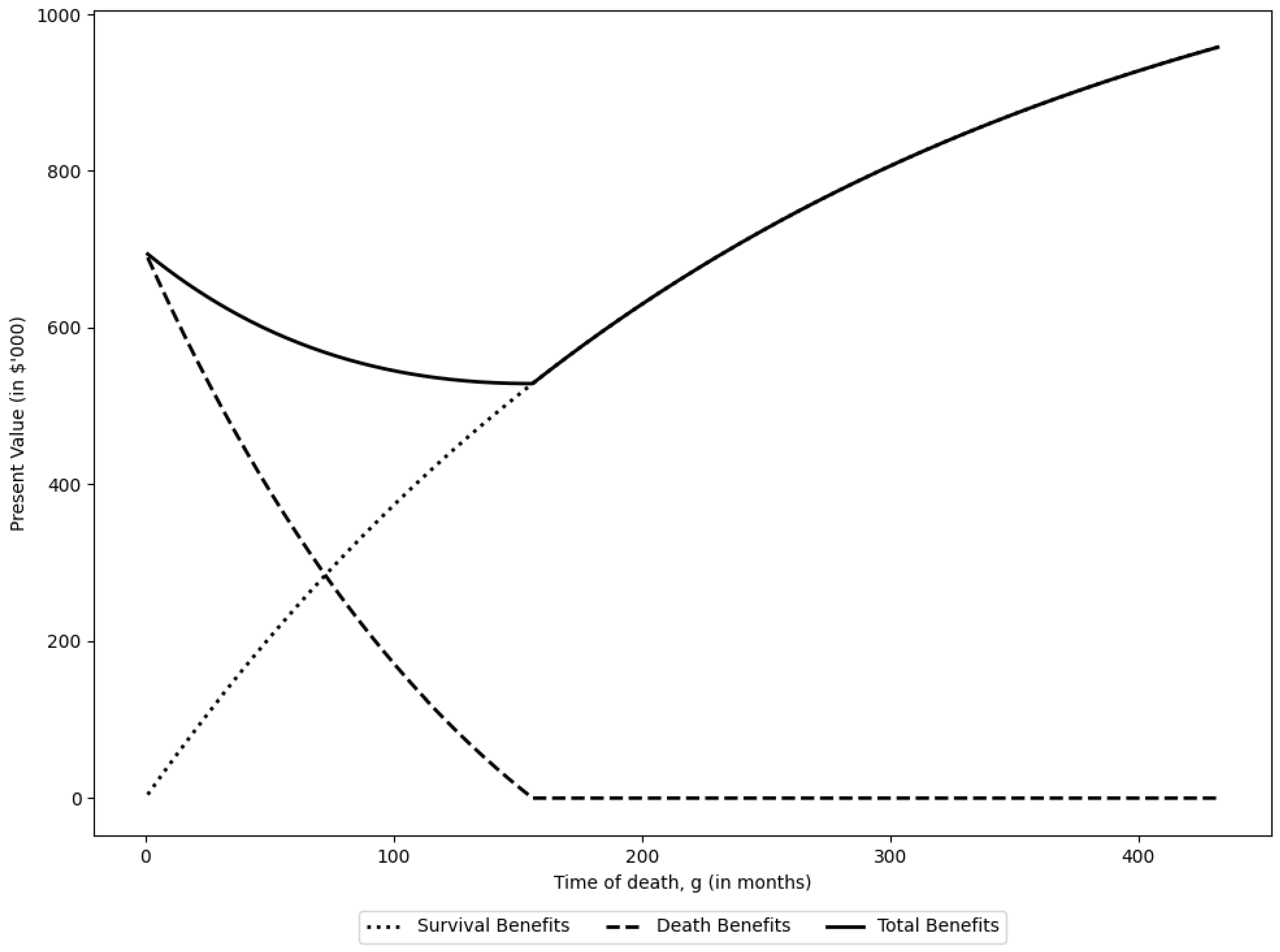
Figure 3 shows the present values of benefits under EHR from the survival benefits
and
and the death benefit
enjoyed by a male homeowner aged 65 versus the time of death with parameters configuration
,
and Singapore mortality experience. As explained in
Section 3.3, the minimum value of the present value of the total benefit is obtained at the expiration time of the decreasing term insurance, which can be identified at the turning point of the total benefit curve in
Figure 3.
5. Conclusions
This study introduces a new Enhanced Home Reversion plan and provides thorough justifications of the major advantages of the new plan over existing sell-type equity release plans. The new plan includes the term life insurance feature to increase the amount of bequest to the owner’s estate, especially when bequest is the main motive. The new plan also provides the hedging effect to minimize the loss of the owner’s principal amount invested under the worst-case early-death scenario. The new features may also be modified to meet the owner’s other needs if necessary. For example, the amount of life annuity payment could be adjusted to inflation effect annually, or the death benefit amount of the term insurance may be reduced to increase the amount of annuity payments. With the flexible features tailored to meet homeowners’ needs, the new enhanced product could stimulate demand for home reversion products from those asset-rich-cash-poor homeowners.
However, we should point out that the supply side is currently limited due to the lack of plan providers willing or able to effectively manage the housing price risk, which could present a major obstacle in the development of sell-type equity release products. Compared with the Reverse Mortgage plan, where providers do not face any housing price risk due to the no-negative equity guarantee insurance, the Home Reversion plan providers are in a difficult position of pricing the products and then managing the housing price risks after the transactions. It is most likely one of the major reasons that explains why loan-type reverse mortgage products are more widely available than sell-type home reversion products, even though the latter with new product features are less complex and more desirable for homeowners. Nevertheless, our study provides the first step to enhancing the demand for sell-type home reversion products by meeting more customers’ needs. The high demand for the products may motivate more Home Reversion plan providers to consider entering the market.


