Abstract
In this paper, we consider the problem of pricing variance, volatility, covariance and correlation swaps for financial markets with semi-Markov volatilities. The paper’s motivation derives from the fact that in many financial markets, the inter-arrival times between book events are not independent or exponentially distributed but instead have an arbitrary distribution, which means they can be accurately modelled using a semi-Markov process. Through the results of the paper, we hope to answer the following question: Is it possible to calculate averaged swap prices for financial markets with semi-Markov volatilities? This question has not been considered in the existing literature, which makes the paper’s results novel and significant, especially when one considers the increasing popularity of derivative securities such as swaps, futures and options written on the volatility index VIX. Within this paper, we model financial markets featuring semi-Markov volatilities and price-averaged variance, volatility, covariance and correlation swaps for these markets. Formulas used for the numerical evaluation of averaged variance, volatility, covariance and correlation swaps with semi-Markov volatilities are presented as well. The formulas that are detailed within the paper are innovative because they provide a new, simplified method to price averaged swaps, which has not been presented in the existing literature. A numerical example involving the pricing of averaged variance, volatility, covariance and correlation swaps in a market with a two-state semi-Markov process is presented, providing a detailed overview of how the model developed in the paper can be used with real-life data. The novelty of the paper lies in the closed-form formulas provided for the pricing of variance, volatility, covariance and correlation swaps with semi-Markov volatilities, as they can be directly applied by derivative practitioners and others in the financial industry to price variance, volatility, covariance and correlation swaps.
1. Introduction
The most basic indicator of a stock’s riskiness or uncertainty is its volatility. Formally, volatility refers to the annualized standard deviation of the stock’s returns during a specified period, with the subscript R denoting the observed or “realized” volatility.
Volatility swaps are forward contracts on future realized stock volatility, while variance swaps are similar contracts on variance, the square of the future volatility. These financial instruments offer investors a convenient means to gain exposure to the future level of volatility.
The most straightforward approach to trade volatility is to utilize volatility swaps, which are also known as realized-volatility forward contracts. This is true, as volatility swaps offer pure exposure to volatility and expose the investor only to volatility.
A covariance swap is a covariance forward contact of two underlying rates and while a correlation swap is a correlation forward contract with the underlying rates and
The literature concerning volatility derivatives is rapidly expanding. Below, we present a concise overview of the most recent developments in this field. Benth et al. (2007) utilized the Non-Gaussian Ornstein–Uhlenbeck stochastic volatility model to investigate volatility and variance swaps. Broadie and Jain (2008a) conducted a comparative analysis of results from different models to explore the impact of jumps and discrete sampling on variance and volatility swaps, while Broadie and Jain (2008b) examined the pricing and hedging strategies for volatility derivatives within the Heston square-root stochastic volatility model. Carr et al. (2005) employed pure jump processes with independent increment return models to price derivatives written on realized variance. Further advancement in this area can be found in Carr and Lee (2007). For a detailed survey on volatility derivatives, we refer to Carr and Lee (2009). Da Fonseca et al. (2011) provided a solution to a portfolio-optimization problem in a market with risky assets and volatility derivatives, and as a result, it was able to produce an analysis of the impact of variance and covariance swaps in a market. An investigation into the price of correlation swaps was conducted by Bossu(2005, 2007) for components of an equity index using the statistical method. The price of correlation risk for equity options is discussed in Driessen et al. (2009). Elliott et al. (2007) delves into the pricing of volatility swaps under Heston’s model with regime switching, while Elliott et al. (2007) explores the pricing of options within a generalized Markov-modulated jump-diffusion model. In Elliott and Swishchuk (2007), formulas for option and swap pricing in a Markov-modulated market are developed, and the minimal martingale measure is explored. The paper Howison et al. (2004) investigates the valuation of different volatility derivatives, covering volatility and variance swaps, as well as options. Sepp (2008) explored the pricing of options based on realized variance within the context of the Heston model, which incorporates jumps in returns and volatility. In Badescu et al. (2002), an extensive analysis of the analytical closed-form pricing formulas for pseudo-variance, pseudo-volatility, pseudo-covariance and pseudo-correlation swaps is conducted. Neuberger (1994) investigated a nonparametric method for swap pricing, which refrained from assuming a specific stochastic process and instead assumed that the price of the underlying evolves continuously over time. Dupire (1993) examined a similar approach to swap pricing while developing the notion of forward variance. A complete and detailed replicating strategy for continuously monitored variance swaps was outlined by Carr and Madan (1999). The groundbreaking concept of localizing variance swap payoffs in space was developed in Dupire (1996) and Derman et al. (1997), independently. In the paper Windcliff et al. (2006), an analysis is conducted regarding the behaviour and hedging strategies concerning volatility derivatives that are observed discretely. The stochastic evolution of a forward interest rate curve was examined within Heath et al. (1992). The modelling and pricing of variance, volatility, covariance and correlation swaps for financial markets with Markov-modulated volatilities were studied in Salvi and Swishchuk (2014). The modelling and pricing of variance and volatility swaps for financial markets with stochastic volatilities in the Heston model were studied in Swishchuk (2004). The modelling and pricing of covariance and correlation swaps for financial markets with semi-Markov volatilities were first studied in Salvi and Swishchuk (2012) and published in Pogorui et al. (2021) (see vol. 2, chp. 5).
Within this paper, we model financial markets featuring semi-Markov volatilities and price-averaged variance, volatility, covariance and correlation swaps for these markets. In many financial markets, the inter-arrival times between book events (e.g., limit orders, market orders and order cancellations) in the limit order books, considering HFT (high-frequency and algorithmic trading), are not independent or exponentially distributed as they would be in the Markov case, but instead, they have an arbitrary distribution (e.g., Weibull, Gamma, etc.). For this reason, we model markets with a semi-Markov process but not a Markov process. In addition, the assumption of the semi-Markov process for modelling swap contracts is appropriate because, within this paper, we consider swap contracts on variance, volatility, covariance and correlation, and the evolution of these statistical measures does not follow the Markov property. Yet the change in variance, volatility, covariance and correlation does follow a semi-Markov process, as is explained in Section 4, using a Weibull distribution.
In the subsequent sections, we present formulas for the numerical evaluation of variance, volatility, covariance and correlation swaps with semi-Markov volatility. The novelty of the paper lies in the closed-form formulas provided for the pricing of averaged variance, volatility, covariance and correlation swaps, as these formulas have not been previously studied in existing literature. In addition, the closed-form formulas for pricing averaged swaps provide a new, simplified and innovative method for derivative practitioners to price swaps, as the formulas can be easily applied by those in the financial industry. Additionally, a numerical example showcasing the pricing of covariance and correlation swaps within a market involving two risky assets is provided.
The paper is organized as follows. Basic definitions for variance, volatility, covariance and correlation swaps are presented in Section 2.1. Section 2.2 covers the definition of a semi-Markov process and explores several of its properties. Section 3.1 investigates variance, volatility, covariance and correlation swaps within financial markets characterized by semi-Markov volatilities. Covariance and correlation swaps for financial markets with semi-Markov volatilities are presented in Section 3.2. Averaged pricing for variance, volatility, covariance and correlation swaps with semi-Markov volatilities are considered in Section 3.3. A numerical example with a two-state semi-Markov process is presented in Section 4. Appendix A considers the first-order approximation for the realized correlation. Section 5 concludes the paper.
2. Basic Definitions and Literature Review
2.1. Variance, Volatility, Covariance, Correlation Swaps: Basic Definitions
Within the following section, we will introduce the definitions and formulas for variance, volatility, covariance and correlation swaps. The formulas and definitions closely follow the information and framework presented in Pogorui et al. (2021) and Salvi and Swishchuk (2012, 2014).
2.1.1. Variance and Volatility Swaps
A stock volatility swap is a forward contract on the annualized volatility. Its payoff at expiration is equal to
where is the realized stock volatility (quoted in annual terms) over the life of contract,
is a stochastic stock volatility, is the annualized volatility delivery price, and N is the notional amount of the swap in dollars per annualized volatility point. The holder of a volatility swap at expiration receives N dollars for every point by which the stock’s realized volatility has exceeded the volatility delivery price . The holder is swapping a fixed volatility for the actual (floating) future volatility . We note that usually, where is a converting parameter such as USD 1 per volatility-square, and I is a long-short index (+1 for long and −1 for short).
Even though volatility is commonly talked about amongst options market participants, variance or volatility squared has more fundamental significance (see Demeterfi et al. 1999).
A variance swap is a forward contract on annualized variance, the square of the realized volatility. Its payoff at expiration is equal to
where is the realized stock variance (quoted in annual terms) over the life of the contract,
is the delivery price for variance, and N is the notional amount of the swap in dollars per annualized volatility point squared. The holder of the variance swap at expiration receives N dollars for every point by which the stock’s realized variance has exceeded the variance delivery price .
Consequently, pricing the variance swap simplifies to computing the square of the realized volatility.
Assessing the value of a variance forward contract or swap follows the same principles as valuing any other derivative security. The forward contract’s value, denoted as P, on the future realized variance with strike price is equal to the expected present value of the future payoff in a risk-neutral world:
where r is the risk-free discount rate corresponding to the expiration date T and E denotes the expectation.
Therefore, in order to calculate the value of variance swaps, we only need to know the mean of the underlying variance, .
However, when we calculate volatility swaps, we need more than just . Within Brockhaus and Long (2000), we can find the Brockhaus–Long approximation (which uses the second-order Taylor expansion for the function ). The Brockhaus–Long approximation can be expressed as follows (see also Javaheri et al. 2002):
where and is the convexity adjustment.
Consequently, in order to calculate the value of volatility swaps, we need to know and
The realized continuously sampled variance is defined in the following way:
The realized continuously sampled volatility is defined as follows:
2.1.2. Covariance and Correlation Swaps
Options that depend on exchange rate movements, particularly those settling in a currency different from the underlying currency, are susceptible to fluctuations in the correlation between the asset and the exchange rate. However, this risk can be mitigated by employing a covariance swap.
A covariance swap is a covariance forward contact of the underlying rates and , and its payoff at expiration is equal to
where is a strike price, N is the notional amount, and is a covariance between two assets and .
A correlation swap is a correlation forward contract with two underlying rates and , and its payoff at expiration is equal to:
where is a realized correlation of two underlying assets and is a strike price, and N is the notional amount.
From a theoretical standpoint, pricing a covariance swap is akin to pricing variance swaps, given that
where and are the two given underlying assets, is the realized variance of the underlying asset S, and is the realized covariance of the two underlying assets and . See Swishchuk (2004) for more details.
Therefore, in order to price a covariance swap we need to know the realized variance for and for
Realized correlation is defined as follows:
where , , and are defined above.
Given two assets and with sampled on days , between today and maturity the logarithmic return of each asset is
Covariance and correlation can be approximated using
and
respectively.
2.2. Semi-Markov Process and Some Properties
The following section describes the semi-Markov process and outlines its properties, closely following the definitions and equations found in Pogorui et al. (2021) and Salvi and Swishchuk (2012, 2014).
Let be a filtered probability space, with a right-continuous filtration and probability .
Let be a measurable space and
be a semi-Markov kernel. Let be an -valued Markov renewal process with as the associated kernel, that is,
Let us then define the process
which gives the number of jumps of the Markov renewal process in the time interval and
which gives the sojourn time of the Markov renewal process in the n-th visited state. The semi-Markov process, associated with the Markov renewal process , is defined by
It is possible to define some auxiliaries processes associated with the semi-Markov process. We are interested in the backward recurrence time (or lifetime) process defined by
The next result characterizes the backward recurrence time process (cf. Swishchuk 2013).
Proposition 1.
The backward recurrence time is a Markov process with generator
where , and .
As is widely acknowledged, semi-Markov processes maintain the lost-memories property solely at transition times, which means that is not a Markov process. Nevertheless, when we examine the joint process , we simultaneously record the duration of time spent by the semi-Markov process in the present state, at any given moment. As a result, is a Markov process with the generator (see Swishchuk 1997)
3. Methods for Pricing Averaged Variance, Volatility, Covariance and Correlations Swaps
3.1. Variance and Volatility Swaps for Financial Markets with Semi-Markov Stochastic Volatilities
Within the section that follows, we will use the formulas and definitions provided in Pogorui et al. (2021) and Salvi and Swishchuk (2012, 2014) to present definitions and equations for variance and volatility swaps in markets with semi-Markov stochastic volatilities.
In the context of a market model involving just two assets, the risk-free bond and the stock, let us suppose that the stock price adheres to the subsequent stochastic differential equation
where w is a standard Wiener process independent of . Our focus lies in examining the characteristics and properties of the volatility, denoted as . The properties of volatility modulated using a Markov process were examined in Salvi and Swishchuk (2012), and here we will generalize their work to the semi-Markov case.
It is widely acknowledged that the market model with semi-Markov stochastic volatility lacks completeness (see Swishchuk 2013). Therefore, to determine the prices of future contracts, we will employ the minimal martingale measure; for details consult Swishchuk (2013). Now, our attention turns to assessing the price of variance, volatility, covariance and correlation swaps with semi-Markov volatilities. As long as the process is a Markov process with generator Q, as defined in Equation (8), then the calculation can be reduced to the Markov case described in Salvi and Swishchuk (2012) and in Pogorui et al. (2021). Here, we present all formulas in the semi-Markov case.
3.1.1. Pricing of Variance Swaps
We shall begin with the simplest swap, the variance swap. Variance swaps are forward contracts on a future realized level of variance. The payoff of a variance swap with an expiration date T is given by
where is the realized stock variance over the life of the contract
is the strike price for the variance swap and N is the notional number of dollars per annualized variance point. We will assume that just for the sake of simplicity. The price of the variance swap is the expected present value of the payoff in the risk-neutral world
The subsequent theorem concerns the assessment of a variance swap within the semi-Markov volatility model. For details and proof, refer to Swishchuk (2013).
Theorem 1
(Swishchuk 2013). The present value of a variance swap with semi-Markov stochastic volatility is
where Q is the generator of ; that is,
3.1.2. Pricing of Volatility Swaps
Volatility swaps are forward contracts on a future realized level of volatility. The payoff of a volatility swap with maturity T is given by
where is the realized stock volatility over the life of the contract
is the strike price for the volatility swap, N is the notional number of dollars per annualized volatility point, and as before, we will assume that . The price of the volatility swap is the expected present value of the payoff in a risk-neutral world
To compute the price of volatility swaps, we require the expected value of the square root of variance. However, in general, this expected value cannot be analytically determined. Therefore, to derive a formula for the price of volatility swaps, an approximation becomes necessary. By employing a similar approach as in the Markov case (see Brockhaus and Long 2000; Javaheri et al. 2002), we use the second-order Taylor expansion, yielding the following expression:
Consequently, in order to assess the price of volatility swaps, it is necessary to determine both the expectation and the variance of . The following theorem provides an explicit representation of the price of a volatility swap, approximated to the second order, within this semi-Markov volatility model. For further details, refer to Salvi and Swishchuk (2012) and Pogorui et al. (2021), vol. 2, chp 5.
Theorem 2.
The value of a volatility swap with semi-Markov stochastic volatility is
where the variance is given by
and Q is the generator of , that is,
3.1.3. Approximations of Variance and Volatility Swaps with Semi-Markov Volatility
When applying the theories and equations presented in Section 3.1.1 and Section 3.1.2 to determine the price of a variance or a volatility swap, we encounter numerical challenges related to Evaluating the family of exponential operators involved in Theorems 1 and 2 above, concerning the semi-Markov stochastic volatility model, is often challenging from a numerical perspective. To address this issue, we initially explore the following identity
for any function . This identity enables us to obtain the operator at any desired order of approximation. For instance, when , we obtain the following expression:
where I is an identity operator. At this order of approximation, we permit the semi-Markov process to undergo a maximum of one transition during the lifetime of the contract. This assumption can be reasonable if we consider the semi-Markov process as a macroeconomic factor. Nevertheless, we can assess the error in this approximation by considering subsequent orders. Employing the first-order approximation, the variance swap price is given by
And the first order of approximation for the volatility swap price becomes
See Salvi and Swishchuk (2012) and Pogorui et al. (2021), vol. 2, chp. 5, for more details.
3.2. Covariance and Correlation Swaps for Financial Markets with Semi-Markov Stochastic Volatilities
In the subsequent section, we will again use the formulas and definitions provided in Pogorui et al. (2021) and Salvi and Swishchuk (2012, 2014) in order to present definitions and equations for covariance and correlation swaps in markets with semi-Markov stochastic volatilities.
Now, let us explore a market model that consists of two risky assets and one risk-free bond. We will assume that the risky assets follow the following stochastic differential equations:
where are deterministic functions of time and , are standard Wiener processes with quadratic covariance given by
where is a deterministic function and are independent of .
In the context of this model, it is valuable to investigate the covariance and correlation swaps concerning the two risky assets.
3.2.1. Pricing of Covariance Swaps
A covariance swap is a covariance forward contract on the underlying assets and , which has a payoff at maturity equal to
where is a strike reference value, N is the notional amount and is the realized covariance of the two assets and given by
The price of the covariance swap is the expected present value of the payoff in a risk-neutral world:
where we set . The subsequent theorem provides a clear and explicit representation of the covariance swap price.
Theorem 3.
The value of a covariance swap with semi-Markov stochastic volatility is
where Q is the generator of , that is,
3.2.2. Pricing of Correlation Swaps
A correlation swap is a forward contract on the correlation between the underlying assets and , which has a payoff at maturity equal to
where is a strike reference value, N is the notional amount and is the realized correlation defined by
where the realized variance is given by
The price of the correlation swap is the expected present value of the payoff in a risk-neutral world, that is
where we set for simplicity. Regrettably, the expected value of is not analytically known. Therefore, in order to obtain a precise formula for the correlation swap price, it becomes necessary to use an approximation. After the approximation, we have the following result (see Salvi and Swishchuk (2012) and Pogorui et al. (2021), vol. 2, chp. 5, for more details):
Theorem 4.
The value of a correlation swap with semi-Markov stochastic volatility is
where Q is the generator of , that is,
3.2.3. Approximations of Covariance and Correlation Swaps with Semi-Markov Stochastic Volatility
To attain more practical expressions for the pricing of covariance and correlation swaps that can be readily applied in numerical examples, we will introduce an approximation for the family of the operator . We will employ a similar approach to the one used for the variance and volatility case, approximating the operators at the first order in Q as
Using this approximation, the covariance swap price becomes
The same approximation then allows us to express the correlation swap price as
See Salvi and Swishchuk (2012) and Pogorui et al. (2021), vol. 2, chp. 5, for more details.
3.3. Averaged Prices of the Variance, Volatility, Covariance and Correlation Swaps with Semi-Markov Volatilities
As was mentioned in Salvi and Swishchuk (2014), the rate of convergence in the approximation of the price depends on the rate of convergence of the transition probabilities matrix of the embedded Markov chain to the stationary distribution (see Salvi and Swishchuk 2012). Moreover, the formulas for the approximations of variance, volatility, covariance and correlation swaps look very ugly, and it is hard to calculate even the first-order correction (see Appendix A below).
That is why we will take the following approach to obtain reasonable formulas for covariance and correlation swaps. We consider the following SDE (GBM in series scheme) for the stock price:
where That is, to improve the approximation, we take in a series scheme, where the semi-Markov process is considered in the long run; i.e., instead of time t, we have Using the averaging principle for an SDE in a series scheme (see Swishchuk 1992, 1997), i.e., weakly, we will obtain the following limiting SDE (averaged GBM):
where
and is the stationary distribution of the embedded Markov chain Of course, here, X is a general state space for the semi-Markov process
In the case of finite or infinite but countable the integrals above become sums or series, respectively. We present the above formulas for the case of a finite state semi-Markov process, i.e.,
Thus, the averaged volatility can be calculated using and (or , and in the finite case). For , we only need to specify some non-exponential distribution In the numerical example below, we show how to do this using the Weibull distribution and a two-state semi-Markov process.
4. Numerical Example: A Semi-Markov Process with Two States
4.1. Defining the Values for Volatilities
Now, how we can define two values for the volatility ? We proceed with the method described in Salvi and Swishchuk (2014), sct. 6. Namely, for each day t, we have access to a high data point and a low data point (say, we use the 500 index for the risky asset prices and the CBOE Volatility Index (VIX) for the volatility). We then interpolate between them, defining , a reference value for day t. By computing the mean of these values, we can subsequently define
If , then the state on day t is denoted as ; otherwise, it is We estimate the transition matrix. The value represents the mean of calculated solely on days in the state, and similarly, is the mean of computed exclusively on days in the state.
4.2. Defining the Values for the Volatilities
How we can define two values for the volatilities ? Here, we proceed with the method described in Salvi and Swishchuk (2014). We employ the S&P 500 index and the NASDAQ-100 index as the two risky assets, denoted as and , respectively. In order to estimate the Markov chain transition matrix and the parameters we utilize the CBOE Volatility Index (VIX) and the CBOE NASDAQ-100 Volatility Index (VXN).
The volatilities of the two assets are influenced by the same Markov chain. Therefore, we can view the two volatility indices as two separate instances of the same process, operating independently.
For each index and a given day t, high data points and low data points are available. We then define a VIX and VXN reference value for day t, by interpolating between the high data points and low data points on each given day
and
We evaluate the mean value over the time period we are interested in. If on day t then VIX is in the state ; otherwise, it is in . Similarly, if then on day t, VXN is in state ; otherwise, it is in state . This process generates two independent sequences of and states of our Markov process: one for VIX and the other for VXN. Utilizing these sequences, we can estimate the transition probability for the Markov chain. Regarding the parameters, can be estimated by taking the mean of all VIX values, , such that t is a day, while can be estimated by taking the mean of all values on which t is a day. Similarly, can be estimated by taking the mean of the and days of VXN, respectively.
4.3. Formulas for the Prices of Averaged Variance, Volatility, Covariance and Correlation Swaps
Below, we present formulas for the prices of averaged variance, volatility, covariance and correlation swaps that follow from the averaged results presented above.
We consider here a two-state case, with In this case, the expressions for averaged volatility m and become
The price of the averaged variance swap is
where is the interest rate, T is the maturity date, and is the strike price.
The price of averaged volatility swap is
The second term in the brackets is usually called the convexity adjustment, and is the strike price.
The price of the covariance swap is
where are volatilities for the risky assets is the strike price, and is the constant correlation between the two Wiener processes in Equation (23).
The price of the correlation swap is
where is the strike price.
4.4. Numerical Toy Example
We will now use the expressions defined above in further calculations below. Suppose that is a Markov chain with two states , and a transition matrix .
Then, the stationary probabilities are which follow from the solution of the following equation:
Therefore, we examine the scenario of a two-state semi-Markov chain with arbitrary distribution for We shall adopt the the Weibull distribution (as detailed in Krishnamoorthy (2006)) denoted as for , which possesses a probability density function represented as
where Recall that represents the shape parameter, while denotes the scale parameter. It is worth noting that if we set then we obtain the exponential distribution for and the Markov case for the process
Suppose that and We recall that the mean value for a random variable with Weibull density distribution is where stands for the Gamma distribution. Of course, we could take other non-exponential distributions, such as Gamma or Beta.
We consider two cases here: (i) and (ii) The case refers to the exponential distribution
Let us take (i)
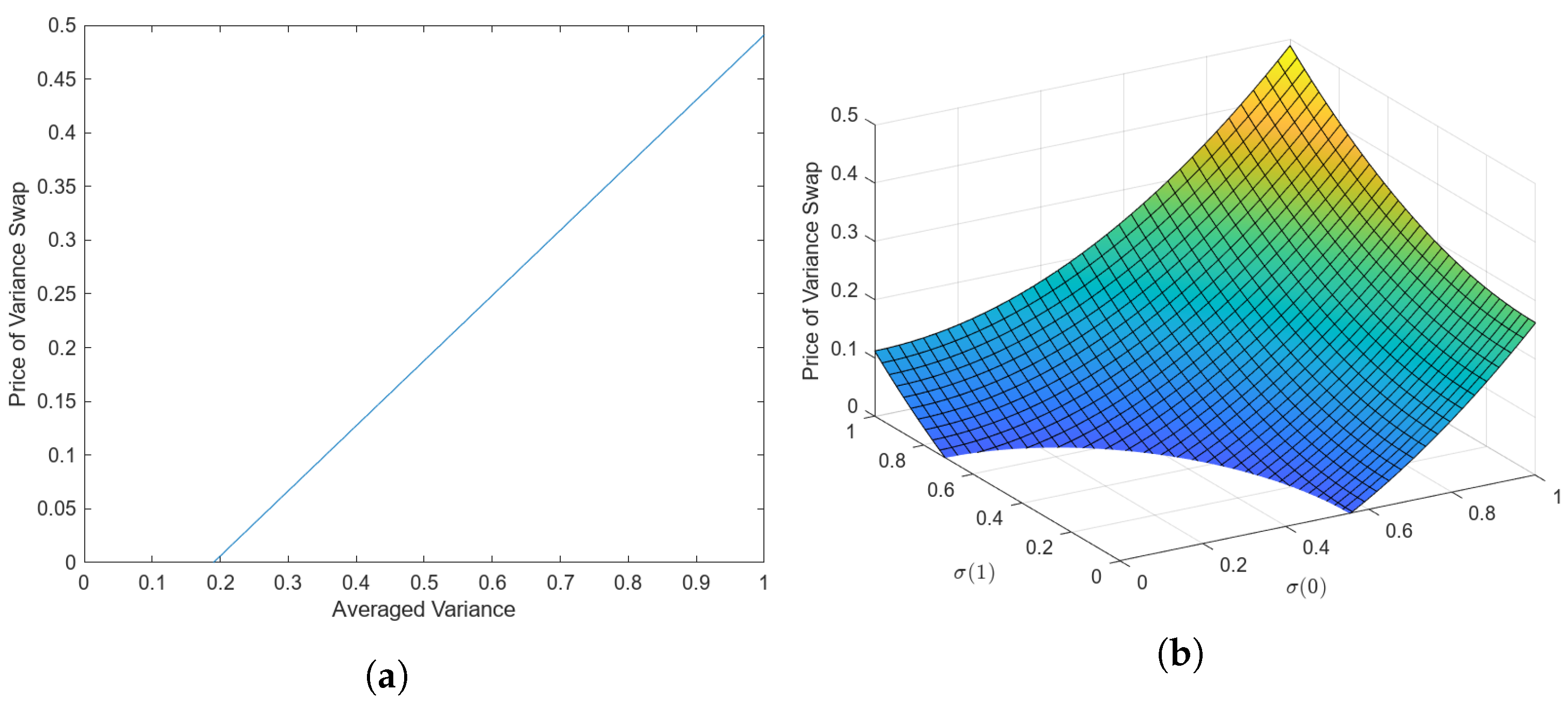
Let us now take Then, the averaged variance is:
It then follows that the averaged variance swap value can be calculated easily using the following formula (we take , and ) (see Equation (46)):
Below, we examine the relationship between the averaged variance and the averaged variance swap price in Figure 1a, as well as the relationship between , and the averaged variance swap price in Figure 1b.

Figure 1.
(a) Price of variance swap in response to changing averaged variance . (b) Price of variance swap in response to changing and .
Similarly, the averaged volatility, covariance and correlation swaps can be calculated using Equations (47)–(49) above, respectively.
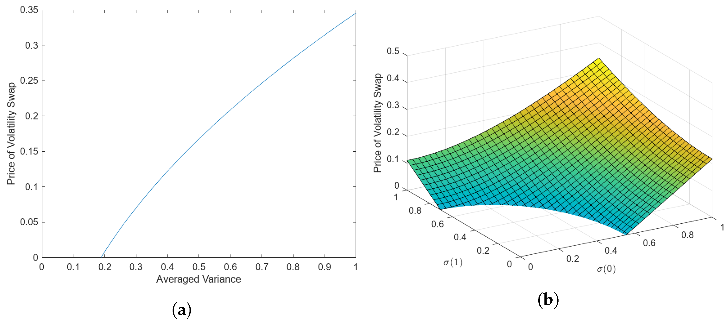
Thus, using formula (47) and we have that the averaged volatility swap value is
We can then examine the relationship between the averaged variance and the averaged volatility swap price in Figure 2a below, as well as the relationship between , and the averaged volatility swap price in Figure 2b.

Figure 2.
(a) Price of volatility swap in response to changing averaged variance . (b) Price of volatility swap in response to changing and .
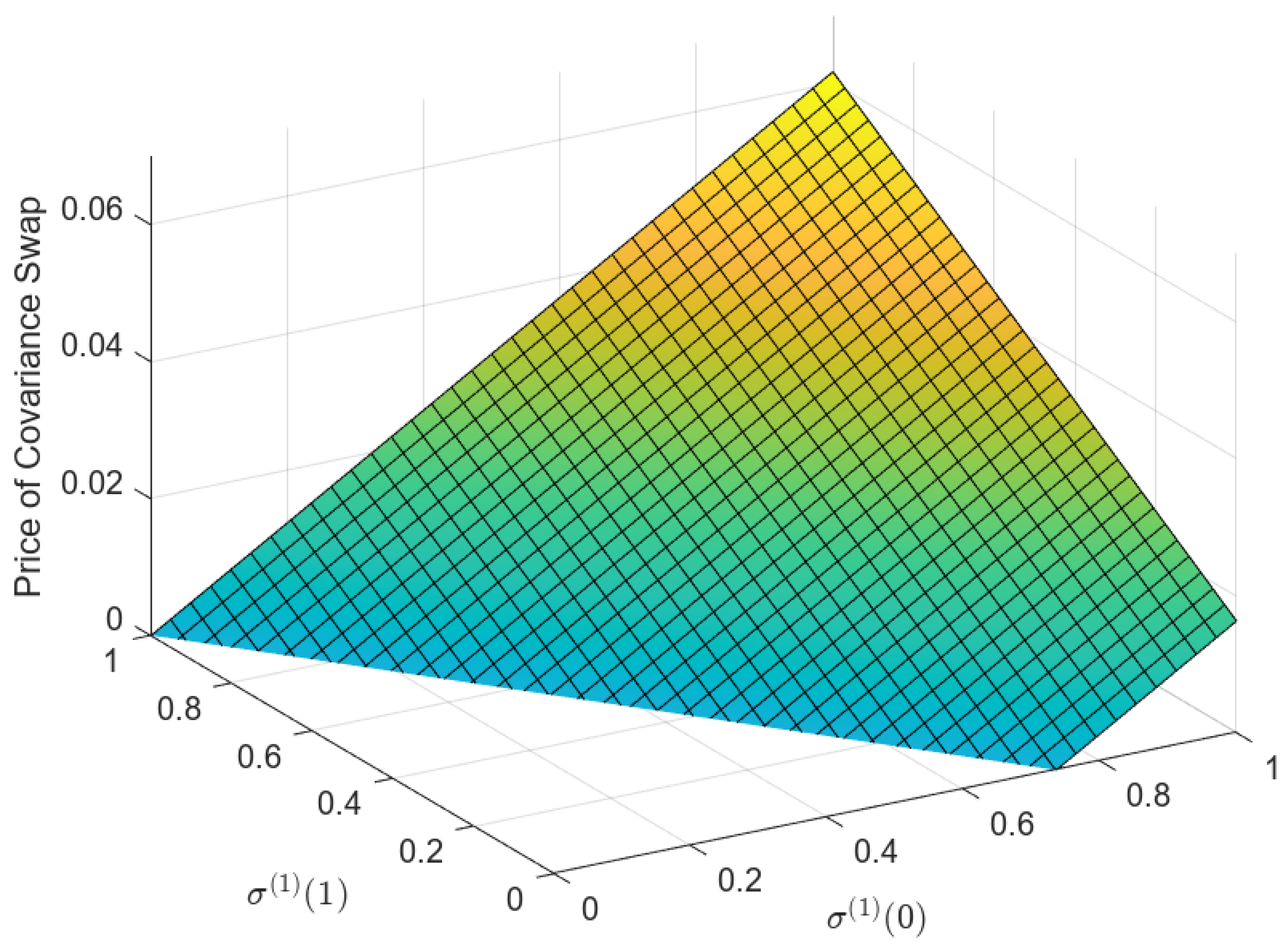
Using the following data, and Equation (48), we can obtain the averaged covariance swap value:
Below, in Figure 3, we examine the relationship between , and the averaged covariance swap value.

Figure 3.
Price of covariance swap in response to changing and .
Again, using the same data, , and Equation (49), we can obtain the averaged correlation swap value:
Below, in Figure 4a, we present a graph that explores the relationship between the averaged variance of the first and second assets and the averaged correlation swap value. In addition, in Figure 4b, a graph is shown that presents the relationship between , and the averaged correlation swap value.
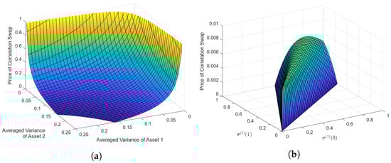
Figure 4.
(a) Price of correlation swap in response to changing averaged variances of assets 1 and 2. (b) Price of correlation swap in response to changing and .
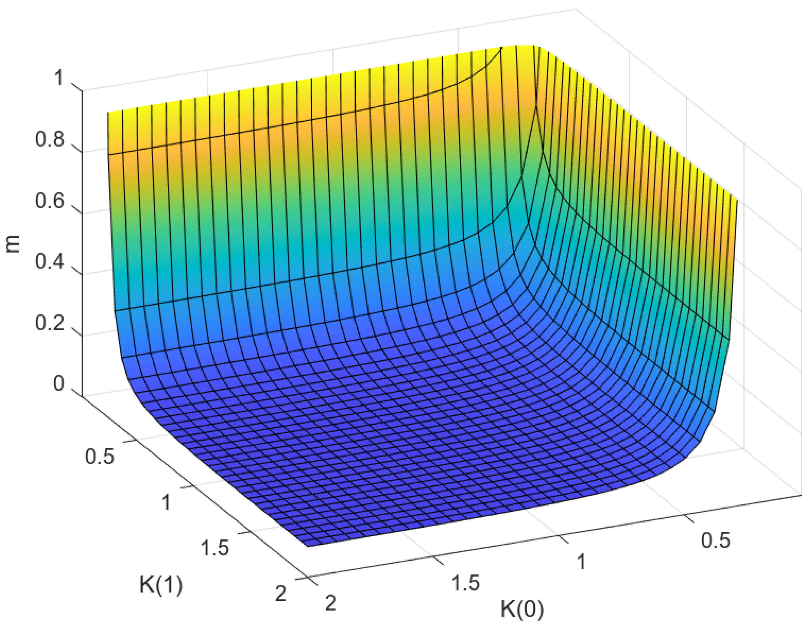
Remark 1.
If we take then we can again calculate the following parameters, and :
And
As we can see from Remark 1 above as well as Figure 5 below, for smaller values of the values of and m are larger and vice versa.

Figure 5.
Relationship between and with m.
5. Conclusions
In this paper, we modelled financial markets with semi-Markov volatilities and determined the pricing of averaged variance, volatility, covariance, and correlation swaps within these market conditions. We also presented formulas for the numerical evaluation of averaged variance, volatility, covariance and correlation swaps with semi-Markov volatilities. A numerical example involving the pricing of averaged variance, volatility, covariance and correlation swaps in a market with a two-state semi-Markov process was presented as well. The paper’s novelty lies in the pricing of averaged variance, volatility, covariance and correlation swaps with semi-Markov volatilities in closed form, as, together with the numerical example, they represent a new contribution to the field of financial derivatives, namely volatility derivatives.
The results of the technical parts of the paper are relevant and important to the financial sector because of the growing popularity and importance of variance, volatility, covariance and correlation swaps. Asset volatility is crucial for the pricing of derivatives, and since the 1990s, a group of derivative securities such as variance swaps have become ever more popular. Since the introduction of the volatility index VIX by the Chicago Board Options Exchange in 1993, swaps, futures, and options written on VIX have become more prominent. As a result, in recent decades, as the trading of swaps written on variance, volatility, covariance and correlation has become more popular, models used to price these swaps have become increasingly relevant and important. In our paper, we used the simplified approach to pricing variance, volatility, covariance and correlation swaps by utilizing averaged statistical measures in a market with semi-Markov volatilities, as was detailed in the numerical example in Section 4, which provides a straightforward approach to pricing swaps that can be used by individuals in the financial industry.
Derivative practitioners can directly apply the results presented in this paper in their work by closely following the information presented in Section 4. Within Section 4.1 and Section 4.2, the definitions for the volatilities to be used are provided, while Section 4.3 outlines the formulas for the pricing of averaged variance, volatility, covariance and correlation swaps. Finally, Section 4.4 details the procedures for the calculation of the swap prices using a numerical toy example. Therefore, a derivative practitioner can directly apply the detailed procedures outlined within Section 4 of the paper to price swaps in their work.
However, due to the lack of literature devoted to averaged swap pricing with semi-Markov volatility, along with the growing popularity of variance, volatility, covariance and correlation swaps, there is an extensive amount of possible future work that can be carried out stemming from the results presented in this paper. In future work, we plan to further research swap pricing by examining volatility swap pricing and the Dupire formula for local semi-Markov volatility. In addition, from the results presented in the paper, one can investigate the residual risk associated with swap pricing.
Overall, the presented results are significant, new and original, and they contribute to advancing our understanding of financial markets associated with semi-Markov volatility and derivative pricing.
Author Contributions
Conceptualization, A.S.; methodology, A.S.; software, S.F.; validation, S.F.; formal analysis, S.F.; investigation, S.F.; data curation, S.F.; writing—original draft preparation, A.S.; writing—review and editing, S.F.; visualization, S.F.; supervision, A.S.; project administration, A.S. All authors have read and agreed to the published version of the manuscript.
Funding
This research received no external funding.
Data Availability Statement
No new data was created or analyzed in this study. Data sharing is not applicable to this article.
Acknowledgments
The authors thank NSERC for continuing support.
Conflicts of Interest
The authors declare no conflict of interest.
Abbreviations
The following abbreviations are used in this manuscript:
| MDPI | Multidisciplinary Digital Publishing Institute |
| S&P 500 | Standard and Poor’s 500 |
| CBOE | Chicago Board Options Exchange |
| VIX | CBOE Volatility Index |
| VXN | CBOE NASDAQ-100 Volatility Index |
| SDE | Stochastic Differential Equation |
| GBM | Geometric Brownian Motion |
| Var | Variance |
| Vol | Volatility |
| Cov | Covariance |
| Corr | Correlation |
| Cf | Confer |
| NSERC | Natural Sciences and Engineering Research Council of Canada |
| HFT | High-Frequency Trading |
Appendix A. Realized Correlation: First Order Correction
In this Appendix, we would like to show what kind of formulas can be obtained without the averaging considered above, closely following the work found in Salvi and Swishchuk (2012). As we will see below, these formulas look very complicated and cannot be calculated exactly or directly. That is why we proposed the approximation method by averaging the swaps under consideration. We take as an example the realized correlation between two assets.
We aim to derive an approximation for the realized correlation between two risky assets
In Salvi and Swishchuk (2014) the following approximated expression was obtained
where
and with the index 0, we have denoted the expected values. We have already calculated the expectation of the zeroth-order approximation, and now we intend to assess the first-order approximation. Substituting X, Y and Z into Equation (A2), we obtain
where
for . We need to calculate the expectation of the right-hand side of Equation (A4). We have already computed the expectation of the first term, which is the zeroth-order approximation for the realized correlation. Therefore, our attention will now shift to the other terms. To begin, let us rewrite them in the following manner:
We have four different contributions in the integrals. The expectation of the terms
for , can be calculated using Theorem 3 in Section 3.2.1. Now, to determine the expectation of the approximated realized correlation, we only need to compute
To this end, let us first divide the range of integration in two intervals as follows
for . We notice that the first integral set is such that , while the second has , so we can use the property of conditional expectation to obtain
We notice that is a Markov process, so using the Markov property, we can express the conditional expectations as
for , and
for . Therefore, the first term of Equation (A10) can be expressed as
while the second term can be expressed as
Now, we can evaluate the functions h and g at x, obtaining
and
We can summarize the preceding result in the following statement, which provides the correlation swap price up to the first order of approximation (for further details, refer to Salvi and Swishchuk (2014)).
Theorem A1.
The value of the correlation swap for a semi-Markov volatility is
where the realized correlation can be approximated by
where Q is the generator of the Markov process given by
As we can see, even with this “approximation”, the Equation (A16) for the realized correlation looks very complicated and hard to calculate, regarding the expression for the generator Q in Equation (A17).
References
- Badescu, Andrei, Anatoliy Swishchuk, Raymond Cheng, Stephan Lawi, Hammouda Mekki, Asrat Gashaw, Yuanyuan Hua, Marat Molyboga, Tereza Neocleous, and Yuri Petratchenko. 2002. Price Pseudo-Variance, Pseudo-Covariance, Pseudo-Volatility, and Pseudo-Correlation Swaps-In Analytical Closed-Forms. Paper presented at the Sixth PIMS Industrial Problems Solving Workshop, University of British Columbia, Vancouver, BC, Canada, May 24–31; pp. 45–55. [Google Scholar]
- Benth, Fred Espen, Martin Groth, and Rodwell Kufakunesu. 2007. Valuing Volatility and Variance Swaps for a Non-Gaussian Ornstein–Uhlenbeck Stochastic Volatility Model. Applied Mathematical Finance 14: 347–63. [Google Scholar] [CrossRef]
- Bossu, Sébastien. 2005. Arbitrage Pricing of Equity Correlation Swaps. Working Paper. London: JPMorgan Equity Derivatives Group. [Google Scholar]
- Bossu, Sebastien. 2007. A New Approach for Modelling and Pricing Correlation Swaps. Working Paper. London: Equity Structuring—ECD. [Google Scholar]
- Broadie, Mark, and Ashish Jain. 2008a. The Effect of Jumps and Discrete Sampling on Volatility and Variance Swaps. International Journal of Theoretical and Applied Finance 11: 761–97. [Google Scholar] [CrossRef]
- Broadie, Mark, and Ashish Jain. 2008b. Pricing and Hedging Volatility Derivatives. The Journal of Derivatives 15: 7–24. [Google Scholar] [CrossRef]
- Brockhaus, Oliver, and Douglas Long. 2000. Volatility Swaps Made Simple. Risk-London Magazine Limited 13: 92–96. [Google Scholar]
- Carr, Peter, Hélyette Geman, Dilip B. Madan, and Marc Yor. 2005. Pricing options on realized variance. Finance and Stochastics 9: 453–75. [Google Scholar] [CrossRef]
- Carr, Peter, and Roger Lee. 2007. Realized Volatility and Variance: Options via Swaps. Technical Report. Chicago: Bloomberg LP and University of Chicago. [Google Scholar]
- Carr, Peter, and Roger Lee. 2009. Volatility Derivatives. Annual Review of Financial Economics 1: 319–39. [Google Scholar] [CrossRef]
- Carr, Peter, and Dilip Madan. 1999. Introducing the Covariance Swap: Techniques for hedging by using the correlation between two currency pairs. Risk 12: 47–51. [Google Scholar]
- Da Fonseca, José, Martino Grasselli, and Florian Ielpo. 2011. Hedging (Co)Variance Risk with Variance Swaps. International Journal of Theoretical and Applied Finance 14: 899–943. [Google Scholar] [CrossRef]
- Demeterfi, Kresimir, Emanuel Derman, Michael Kamal, and Joseph Zou. 1999. A Guide to Volatility and Variance Swaps. The Journal of Derivatives 6: 9–32. [Google Scholar] [CrossRef]
- Derman, Emanuel, Iraj Kani, and Michael Kamal. 1997. Trading and hedging local volatility. Journal of Financial Engineering 6: 233–68. [Google Scholar]
- Driessen, Joost, Pascal J. Maenhout, and Grigory Vilkov. 2009. The Price of Correlation Risk: Evidence from Equity Options. The Journal of Finance 64: 1377–406. [Google Scholar] [CrossRef]
- Dupire, Bruno. 1993. Model Art. Risk 6: 118–24. [Google Scholar]
- Dupire, Bruno. 1996. A unified theory of volatility. In Derivatives Pricing: The Classic Collection. London: Risk Books, pp. 185–96. [Google Scholar]
- Elliott, Robert J., Tak Kuen Siu, and Leunglung Chan. 2007. Pricing Volatility Swaps Under Heston’s Stochastic Volatility Model with Regime Switching. Applied Mathematical Finance 14: 41–62. [Google Scholar] [CrossRef]
- Elliott, Robert J., Tak Kuen Siu, Leunglung Chan, and John W. Lau. 2007. Pricing Options Under a Generalized Markov-Modulated Jump-Diffusion Model. Stochastic Analysis and Applications 25: 821–43. [Google Scholar] [CrossRef]
- Elliott, Robert J., and Anatoliy V. Swishchuk. 2007. Pricing Options and Variance Swaps in Markov-Modulated Brownian Markets. In Hidden Markov Models in Finance. Edited by Rogemar S. Mamon and Robert J. Elliott. Series Title: International Series in Operations Research & Management Science; Boston: Springer US, vol. 104, pp. 45–68. [Google Scholar] [CrossRef]
- Heath, David, Robert Jarrow, and Andrew Morton. 1992. Bond pricing and the term structure of interest rates: A new methodology for contingent claims valuation. Econometrica: Journal of the Econometric Society 60: 77–105. [Google Scholar] [CrossRef]
- Howison, Sam, Avraam Rafailidis, and Henrik Rasmussen. 2004. On the pricing and hedging of volatility derivatives. Applied Mathematical Finance 11: 317–46. [Google Scholar] [CrossRef]
- Javaheri, Alireza, Paul Wilmott, and Espen Haug. 2002. GARCH and Volatility swaps. Quantitative Finance 4: 589–595. [Google Scholar] [CrossRef]
- Krishnamoorthy, Kalimuthu. 2006. Handbook of Statistical Distributions with Applications. Number 188 in Statistics, a Series of Textbooks & monographs; Boca Raton: Chapman & Hall/CRC. [Google Scholar]
- Neuberger, Anthony. 1994. The Log Contract. The Journal of Portfolio Management 20: 74–80. [Google Scholar] [CrossRef]
- Pogorui, Anatoliy, Anatoliy Swishchuk, and Ramón M. Rodríguez-Dagnino. 2021. Random Motions in Markov and Semi-Markov Random Environments 2: High-dimensional Random Motions and Financial Applications, 2nd ed. New York: John Wiley & Sons. [Google Scholar]
- Salvi, Giovanni, and Anatoliy Swishchuk. 2014. Covariance and Correlation Swaps for Financial Markets with Markov-Modulated Volatilities. International Journal of Theoretical and Applied Finance 17: 1–23. [Google Scholar] [CrossRef]
- Salvi, Giovanni, and Anatoliy V. Swishchuk. 2012. Modeling and Pricing of Covariance and Correlation Swaps for Financial Markets with Semi-Markov Volatilities. arXiv arXiv:1205.5565. doi:10.48550/ARXIV.1205.5565. [Google Scholar] [CrossRef]
- Sepp, Artur. 2008. Pricing options on realized variance in heston model with jumps in returns and volatility. Journal of Computational Finance 11: 33–70. [Google Scholar] [CrossRef]
- Swishchuk, Anatoliy. 1992. Limit theorems for stochastic differential equations with semi-Markov switchings. Paper presented at the the International School-Evolution of Stochastic Systems: Theory and Applications, Ukraine, Crimea, May 3; pp. 3–4. [Google Scholar]
- Swishchuk, Anatoly. 1997. Random Evolutions and Their Applications. Number 408. Dordrechts: Kluwer Academic Publishers. [Google Scholar]
- Swishchuk, Anatoliy. 2004. Modeling of Variance and Volatility Swaps for Financial Markets with Stochastic Volatilities. Wilmott Magazine 2: 64–72. [Google Scholar]
- Swishchuk, Anatoliy. 2013. Pricing of Variance and Volatility Swaps with Semi-Markov Volatilities. Singapore: World Scientific Publishing Co. Pte. Ltd., pp. 173–87. [Google Scholar]
- Windcliff, Heath, Peter Forsyth, and Ken Vetzal. 2006. Pricing methods and hedging strategies for volatility derivatives. Journal of Banking & Finance 30: 409–31. [Google Scholar] [CrossRef]

Disclaimer/Publisher’s Note: The statements, opinions and data contained in all publications are solely those of the individual author(s) and contributor(s) and not of MDPI and/or the editor(s). MDPI and/or the editor(s) disclaim responsibility for any injury to people or property resulting from any ideas, methods, instructions or products referred to in the content. |
© 2023 by the authors. Licensee MDPI, Basel, Switzerland. This article is an open access article distributed under the terms and conditions of the Creative Commons Attribution (CC BY) license (https://creativecommons.org/licenses/by/4.0/).