On the Diversification Effect in Solvency II for Extremely Dependent Risks

Abstract

In this article, we investigate the validity of diversification effect under extreme-value copulas, when the marginal risks of the portfolio are identically distributed, which can be any one having a finite endpoint or belonging to one of the three maximum domains of attraction. We show that Value-at-Risk (V@R) under extreme-value copulas is asymptotically subadditive for marginal risks with finite mean, while it is asymptotically superadditive for risks with infinite mean. Our major findings enrich and supplement the context of the second fundamental theorem of quantitative risk management in existing literature, which states that V@R of a portfolio is typically non-subadditive for non-elliptically distributed risk vectors. In particular, we now pin down when the V@R is super or subadditive depending on the heaviness of the marginal tail risk. According to our results, one can take advantages from the diversification effect for marginal risks with finite mean. This justifies the standard formula for calculating the capital requirement under Solvency II in which imperfect correlations are used for various risk exposures.

1. Introduction

Measuring the risk of a portfolio of losses is crucial for the computation of total capital requirement within the Solvency II and Basel II/III regulatory frameworks. In fact, the Solvency Capital Requirement (SCR) in the framework of Solvency II is calculated by combining a number of separate risk modules (e.g., market risk, default risk, life risk, health risk, non-life risk) with linear correlation techniques and corresponds to V@R of the basic own funds of an (re)insurance undertaking subject to a confidence level of $99.5\%$ over a one-year time horizon, taking into account the dependencies within and across risk categories (see Pfeifer and Strassburger 2008; Sandström 2007; Vesa et al. 2007). To be more specific, if the capital requirement of different risk categories, $SC{R}_i$, and the correlation factors, $Cor{r}_{i,j}$, for these risks are provided, together with the intangible asset risk, $SC{R}_{intangible}$, the basic solvency capital requirement (BSCR) can be obtained with the following formula,

$$BSCR=\sqrt{\sum _{ij}Cor{r}_{i,j}\times SC{R}_i\times SC{R}_j}+SC{R}_{intangible}.$$

The capital requirement of operation risk and an adjustment are then added to BSCR to obtain the overall SCR. Even though simple models such as correlation matrices are adopted by Solvency II, the characteristics of V@R under more complicated dependence structures are still worth further study. V@R is also the risk measure adopted by Basel II/III in assessing the market risk, operational risk, and counterparty credit risk. More precisely, given a collection of d loss random variables, $X_i$, for $i=1,\dots d$, it is of practical interest for the financial institutions to find the total capital requirement, C, as

$$C=\delta \sum _{i=1}^d\mathrm{V}@{\mathrm{R}}_p\left(X_i\right),$$

for some $\delta >0$ and p close to 1. To reflect the effect of diversification, the multiplication factor, $\delta$, is usually taken to be less than 1. In the Basel III accord, the capital multipliers are set to be between 3 and 4 to address the issue of model uncertainty.

Under some specific situations, for example, when the risks are elliptically distributed, V@R is shown to be a coherent risk measure for confidence level $p\ge 0.5$; see Embrechts et al. (2009a) for more details. However, V@R is generally neither subadditive nor superadditive; this negative result is coined as the second fundamental theorem of quantitative risk management in Embrechts (2000), which states that V@R is typically non-subadditive for non-elliptically distributed risk vectors. To fill in a more precise context of this statement, any sufficient conditions for sub-additivity or super-additivity is much welcome. It is a well-known fact that comonotonicity warrants the additivity of V@R. Motivated by intensive discussion concerning the appropriate way to measure the operational risk, Embrechts et al. (2009b) studied the asymptotic additivity of V@R of multivariate-dependent risks under the Archimedean copulas, where all the risks are identically distributed with regular variation, and they showed that either super- or sub-additivity is plausible. It is superadditive when the regularly varying index is less than one, and subadditive when the index is greater than one. Hua and Joe (2012) investigated the properties of upper/lower tail comonotonicity that can be applied to absolutely continuous distributions, and proved the asymptotic additivity of V@R for random variables that are in the Maximum Domain of Attraction (MDA) of either Fréchet or Gumbel under the assumptions of tail comonotonicity and tail equivalence. Cheung et al. (2019) showed the universal asymptotic additivity of V@R for a portfolio under the upper tail comonotonicity, in which each marginal risk could be any one having a finite endpoint or belonging to one of the three MDAs, and they are not necessarily identically distributed nor tail equivalent.

It is challenging to construct multivariate distributions which can properly describe the dependence structure among a basket of risks. Indeed, while the marginal distributions are easy to estimate as their data are relatively abundant, the dependence structure among these variables is much harder to calibrate. People often resort to copulas, especially the parametric ones with relatively few parameters, to model the dependence structure directly. Applications of copulas are widely found in various fields, such as actuarial science, quantitative finance, econometrics, and environmetrics. In particular, the statistical modeling of the joint tail distributions attracts most attention, in which multivariate extremes also play a vital role. Standard general references for copula modeling and studies on multivariate extremes can be found in the works of Beirlant et al. (2006), Cherubini et al. (2011), de Haan and Ferreira (1999), Denuit et al. (2005), Falk et al. (2010), Joe (1997), Nelsen (2006), and Resnick (2013).

After various financial crises, researchers and practitioners became more aware of the significance of modeling the dependence in the joint tails using appropriate copulas. For example, Pfeifer and Ragulina (2018, 2021) proposed different copula models generating the unfavourable V@R scenarios that can be used in the stress tests under Solvency II. The joint probability of defaults would be underestimated if one uses copulas that cannot capture the usual tail dependence, which may cause large losses at the portfolio level and adversely affect the solvency of financial institutions; more details can be found in some empirical studies and aftermath analyses of the financial crises, e.g., Alm (2016), Poon et al. (2004). Along with the strict requirements of Solvency II and the increasing complexity of (re)insurance products, flexible enough copulas with sufficient mathematical tractability and the ability of capturing a wide range of tail dependence structures are much desired in both academia and industry. As a representative example, the family of extreme-value copulas forms a rich enough semi-parametric yet manageable class of copulas with positive association; see Beirlant et al. (2006). These copulas originate from the dependence structures of multivariate generalized extreme value (GEV) distributions. They stand for the limiting distributions of the component-wise maxima of the marginal random vectors after normalization. The first monograph of multivariate extreme-value dependence can date back to the work of Galambos (1978). Extreme-value copulas have been studied extensively in Beirlant et al. (2006), in which they described both parametric and non-parametric techniques of the estimation of the multivariate extreme-value dependence structure. Decent summaries on bivariate and multivariate extreme-value copulas can also be found in Gudendorf and Segers (2010), Joe (2014), and Kotz and Nadarajah (2000).

To name a few commonly used extreme-value copulas, for instance, the Gumbel–Hougaard copula is the only one which is also Archimedean (Genest and Rivest 1989). Some other examples include the Galambos, the Hüsler–Reiss, and the t-EV copulas. In particular, the Galambos copula was obtained by Galambos (1975) as an extreme-value limit of the multivariate Pareto distribution, with the Clayton copula as a survival copula. The t-EV copula is the limiting copula of the component-wise maxima of t-distributed random vectors (Demarta and McNeil 2005). The Hüsler–Reiss copula is the limiting extreme-value copula of multivariate t-copulas as its degrees of freedom tend to infinity (Nikoloulopoulos et al. 2009). Plenty of works are devoted to the construction of other parametric families of extreme-value copulas. For example, Asimit and Jones (2007) constructed an extreme-value copula by considering the limiting upper copula of bivariate elliptical distributions. Hua (2017) proposed a two-parameter bivariate copula family which has a full-range tail dependence for both upper and lower tails, and also obtained the corresponding extreme-value copula. Other similar constructions with extension can be found in Su and Hua (2017).

Generally speaking, an extreme-value copula is characterized by its Pickands dependence function, which is a function on the unit simplex subject to certain shape constraints (refer to Equation (5) for the explicit form) that arise from an integral transform of the underlying spectral measure (see Beirlant et al. 2006 for more details). The non-parametric estimator of the Pickands dependence function was developed in Pickands (1981), while its extensions can be found in Hall and Tajvidi (2000). Extreme-value copulas are of increasing practical interest in finance and insurance. For the risk management in the fields of finance (McNeil et al. 2005) and insurance (Frees and Valdez 1998), the computation of V@R is demanded by the regulations in accordance with Solvency II and Basel Accords II/III; this is crucial for financial stability and is the focus of this article.

In this paper, we aim to investigate the validity of the diversification effect for dependent risks by extending the study of the asymptotic sub/super-additivity of V@R. We focus on risks with identical distribution belonging to one of the three MDAs or having a finite endpoint, and their dependence structure is specified by extreme-value copulas. More specifically, we show that V@R is asymptotically subadditive for risks with the common distribution coming from the Gumbel and Weibull MDAs. Moreover, we prove that whether V@R is asymptotically subadditive, additive, or superadditive depends on the value of the regularly varying index if the common distribution is from the Fréchet MDA. In general, the diversification effect is confirmed for the marginal risks with finite mean. While these results are a kind of folklore in the fields of extreme value theory and quantitative risk management, their precise mathematical statements and illustrations have been absent in the literature due to its non-trivial nature. This article fills this gap by providing a precise and systematic analysis on the topic. Our key results complement the second fundamental theorem of quantitative risk management by adding a broad sufficient condition for sub/super-additivity. It is also worth mentioning that the SCR is calculated by combining a number of individual risk modules, allowing for diversification credits by means of correlation matrices or other methodologies. According to our results, one can take advantages from diversification for insurable marginal risks with finite mean. This justifies the standard formula for calculating the capital requirement under Solvency II.

The rest of this article is organized as follows. Section 2 gives a review on some useful concepts and results related to extreme-value theory and copulas. Section 3 presents our major theorems, particularly in Section 3.2, Section 3.3 and Section 3.4, where we consider the asymptotic sub/super-additivity for distributions from the Gumbel, Weibull, and Fréchet MDAs, respectively. Several comprehensive numerical illustrations are provided in Section 4. These simulation studies demonstrate that the effect of the common marginal distribution on the tail behaviour of their sum is stronger than that imposed by their dependence structure. Section 5 concludes our results in the article.

2. Preliminaries

2.1. Overview of Extreme Value Theory

Let $X_1,\dots ,X_n$ be independent and identically distributed (i.i.d.) non-degenerate random variables and denote their maximum by $M_n:=max\{X_1,\dots ,X_n\}$. Given two distributions functions, $F\left(x\right)$ and $G\left(x\right)$, they are of the same type if there exist $a>0$ and $b\in \mathbb{R}$ such that $F\left(x\right)=G(ax+b)$ for all $x\in \mathbb{R}$. Here, we introduce an important result of the extreme value theory.

Theorem 1.

Let $\left\{X_n\right\}$ be a sequence of i.i.d. random variables. If there exist norming constants $a_n>0$ and $b_n\in \mathbb{R}$, for $n=1,2,\dots ,$ and some non-degenerate distribution function $V\left(x\right)$ such that

$$\mathbb{P}(M_n\le a_{n}x+b_n)\to V\left(x\right),$$

(1)

then $V\left(x\right)$ belongs to one of the following three types of distribution functions: for $\alpha >0$,

$$\begin{array}{ccc}\hfill Gumbel:\Lambda \left(x\right)& =& exp\{-e^{-x}\},x\in \mathbb{R};\hfill \\ \hfill Weibull:{\Psi }_{\alpha }\left(x\right)& =& \left\{\begin{array}{cc}exp\{-{(-x)}^{\alpha }\},\hfill & x<0,\hfill \\ 1,\hfill & x\ge 0;\hfill \end{array}\right.\hfill \\ \hfill Fréchet:{\Phi }_{\alpha }\left(x\right)& =& \left\{\begin{array}{cc}0,\hfill & x\le 0,\hfill \\ exp\{-x^{-\alpha }\},\hfill & x>0.\hfill \end{array}\right.\hfill \end{array}$$

These three distributions are called extreme value distributions. We say that a random variable, X, belongs to the Maximum Domain of Attraction (MDA) of the extreme value distribution, $V=\Lambda ,$${\Psi }_{\alpha }$, or ${\Phi }_{\alpha }$ (Gumbel, Weibull, or Fréchet distribution, respectively), if there exist constants $a_n>0,b_n\in \mathbb{R}$, for $n=1,2,...$, such that (1) holds. We also write it as $X\in \mathrm{MDA}\left(V\right)$. The three MDAs cover essentially all the distributions that are of interest in finance, insurance, and quantitative risk management. As a brief introduction of the characteristics of the three MDAs, distributions in $\mathrm{MDA}\left({\Phi }_{\alpha }\right)$ have the heaviest tail. Distributions in $\mathrm{MDA}(\Lambda )$ are the intermediate cases, which can have a finite or an infinite endpoint. Distributions in $\mathrm{MDA}\left({\Psi }_{\alpha }\right)$ are light-tailed and have a finite endpoint. Through out this paper, we use $x_F$ to denote the endpoint of a distribution for easy communication, i.e., the distributoin has a measure of 0 whenever $x>x_F$.

Furthermore, the underlying distribution function of the risk can also be used to identify the class of MDA to which it belongs. Denote the survival function of F by $\overline{F}$. A distribution, F, lies in $\mathrm{MDA}\left(V\right)$ with norming constants $a_n>0$ and $b_n\in \mathbb{R}$ if and only if ${lim}_{n\to \infty }n\overline{F}(a_{n}x+b_n)=-lnV\left(x\right)$ for any $x\in \mathbb{R}$, where the right-hand side is interpreted as ∞ if $V\left(x\right)=0$.

For a non-decreasing function, h on $\mathbb{R}$, we denote the generalized inverse of h by

$$h^{\leftarrow }\left(t\right):=inf\{u\in \mathbb{R}:h\left(u\right)\ge t\}.$$

Then, we can have the following choices of the norming constants. Their derivations can also be found in Embrechts et al. (2013) and Resnick (2013).

Proposition 1.

For a distribution $F\in \mathrm{MDA}\left(V\right)$, the norming constants can be chosen as:

1. 

if $V=\Lambda$, take $a_n=a\left(b_n\right)$ and $b_n={\left(1/\overline{F}\right)}^{\leftarrow }\left(n\right)$, where the function a is

$$a\left(x\right)={\int }_x^{x_F}\frac{\overline{F}\left(u\right)}{\overline{F}\left(x\right)}du,x<x_F;$$

2. 

if $V={\Psi }_{\alpha }$, take $a_n=x_F-{\left(1/\overline{F}\right)}^{\leftarrow }\left(n\right)$ and $b_n=x_F$;

3. 

if $V={\Phi }_{\alpha }$, take $a_n={\left(1/\overline{F}\right)}^{\leftarrow }\left(n\right)$ and $b_n=0$.

These representations of norming constants will be used in our proofs of the main results.

2.2. Copulas

Copula has been a popular tool in financial and insurance industries and can be used to identify the potential statistical arbitrage opportunities in the financial markets and the dependence structure among various risks faced by the insurance companies. More applications can be found in standard references for quantitative risk management, such as McNeil et al. (2005). In this subsection, we provide a quick review on the theory of copulas, especially the extreme-value copula, which motivates our work in the coming section. More details on the theory of copulas and extreme-value copulas can be found in Gudendorf and Segers (2012), Joe (1997), and Nelsen (2006).

A d-dimensional copula is a multivariate distribution on ${[0,1]}^d$ with the standard uniform marginals. For a d-dimensional distribution function, F, with the marginals $F_1,\dots ,F_d$, in accordance with Sklar’s theorem (see Theorem 2.10.9 in Nelsen 2006), one can find a d-dimensional copula C such that for all $\mathbf{x}=(x_1,\dots ,x_d)\in {\mathbb{R}}^d$, we have an alternative representation of:

$$F(x_1,x_2,\dots ,x_d)=\mathbb{P}(X_1\le x_1,\dots ,X_d\le x_d)=C(F_1\left(x_1\right),F_2\left(x_2\right),\dots ,F_d\left(x_d\right)).$$

(2)

For any copula C satisfying (2), we call it a copula of F or a copula of random vector $\mathbf{X}$. In addition, if all the marginal distributions, $F_1,\dots ,F_d$, are continuous, the copula C is unique. From the expression of Equation (2), we can see that the copula demonstrates the dependence structure between the underlying random variables.

Equation (2) focuses on the joint distribution of the lower tail. Here, we introduce its upper tail counterpart, which is relevant to our discussion on upper tail dependence structure. It is known as the survival copula. For any random vector, $\mathbf{X}$, we define the survival copula of $\mathbf{X}$ by $\widehat{C}$, where

$$\widehat{C}({\overline{F}}_1\left(x_1\right),\dots ,{\overline{F}}_d\left(x_d\right)):=\mathbb{P}(X_1>x_1,\dots ,X_d>x_d),\mathbf{x}\in {\mathbb{R}}^d.$$

For the survival copula $\widehat{C}$, we further have $\widehat{C}(u_1,\dots ,u_d)=\overline{C}(1-u_1,\dots ,1-u_d)$ where

$$\overline{C}(u_1,\dots ,u_d):=1+\sum _{\mathcal{J}\subset \{1,\dots ,d\}}{(-1)}^{\left|\mathcal{J}\right|}{C}_{\mathcal{J}}(u_i,i\in \mathcal{J}),$$

and $C_{\mathcal{J}}$ is the $\mathcal{J}$-margin of the copula C with $\left|\mathcal{J}\right|$ being the cardinality of the subset $\mathcal{J}$.

Now, we introduce the family of extreme-value copulas, whose first construction dates back to Deheuvels (1984) and Galambos (1978). The following definition and representation of extreme-value copulas are adapted from Gudendorf and Segers (2010, 2012).

Definition 1.

A copula C is called an extreme-value copula if there exists a copula $C_F$ such that

$$\begin{array}{c}\hfill C_F^n(u_1^{1/n},\dots ,u_d^{1/n})\to C(u_1,\dots ,u_d)\mathrm{as}n\to \infty ,\end{array}$$

(3)

for all $(u_1,\dots ,u_d)\in {[0,1]}^d$. Moreover, the copula $C_F$ is said to be in the domain of attraction of C.

A d-dimensional copula C is max-stable if it satisfies $C(u_1,\dots ,u_d)=C^m(u_1^{1/m},\dots ,u_d^{1/m})$ for all integers $m\ge 1$ and all $(u_1,\dots ,u_d)\in {[0,1]}^d$. A max-stable copula is in its own domain of attraction and so is an extreme-value copula itself. To show that extreme-value copulas are max-stable, consider a fixed integer, $m\ge 1$ and $n=mk$; clearly $n\to \infty$ as $k\to \infty$. Moreover,

$$\begin{array}{cc}& C_F^n(u_1^{1/n},\dots ,u_d^{1/n})=C_F^{mk}(u_1^{1/mk},\dots ,u_d^{1/mk})\to C^m(u_1^{1/m},\dots ,u_d^{1/m})\mathrm{as}k\to \infty ,\mathrm{while}\\ & C_F^n(u_1^{1/n},\dots ,u_d^{1/n})\to C(u_1,\dots ,u_d)\mathrm{as}n\to \infty .\end{array}$$

Hence, a copula is an extreme-value copula if and only if it is max-stable.

To introduce more on the properties of extreme-value copulas, let ${\mathbb{S}}_{d-1}=\{(w_1,\dots ,w_d)\in {[0,\infty )}^d:{\sum }_j{w}_j=1\}$ be the unit simplex in ${\mathbb{R}}^d$. We provide an alternative expression of the extreme-value copula given by Gudendorf and Segers (2012), where the result is in turn adapted from de Haan and Resnick (1977) and Pickands (1981).

Proposition 2.

(Theorem 2.2 of Gudendorf and Segers 2012). A d-dimensional copula C is an extreme-value copula if and only if there exists a finite Borel measure H on ${\mathbb{S}}_{d-1}$, called spectral measure, such that

$$C(u_1,\dots ,u_d)=exp(-l(-ln{u}_1,\dots ,-ln{u}_d)),(u_1,\dots ,u_d)\in {(0,1]}^d,$$

where the tail dependence function, $l:{[0,\infty )}^d\to [0,\infty )$, is given by

$$\begin{array}{c}\hfill l(x_1,\dots ,x_d)={\int }_{{\mathbb{S}}_{d-1}}\stackrel{d}{\underset{j=1}{\bigvee }}\left(w_j{x}_j\right)dH(w_1,\dots ,w_d),(x_1,\dots ,x_d)\in {[0,\infty )}^d.\end{array}$$

(4)

The spectral measure, H, is arbitrary, except for the following d moment constraints

$$\begin{array}{c}\hfill {\int }_{{\mathbb{S}}_{d-1}}{w}_{j}dH(w_1,\dots ,w_d)=1,j\in \{1,\dots ,d\}.\end{array}$$

(5)

This expression will be used in deriving the our main results in Section 3.

3. Model Setting and Main Results

3.1. Dependence Structure

Let $X_1,\dots ,X_d\ge 0$ be loss random variables defined on a probability space $(\Omega ,\mathcal{F},\mathbb{P})$ for a fixed $d\ge 2$. We assume that $X_1,\dots ,X_d$ have the same continuous marginal distribution function, F, and their dependence structure is specified by a d-variate extreme-value copula. Some examples of extreme-value copulas can be found in Table 1. In general, when the risks are not identically distributed, the risk with the heaviest tail dominates the others and determines the tail characteristics of the aggregated risk (see Cheung et al. 2019 for more details).

Table 1. Examples of extreme-value copulas.

Name of Copula	d-Variate Form $\mathit{C}({\mathit{u}}_1,\cdots ,{\mathit{u}}_{\mathit{d}})$	Note
Gumbel–Hougaard	$exp\left[-{\left({\left(-ln{u}_1\right)}^{\alpha }+\cdots +{\left(-ln{u}_d\right)}^{\alpha }\right)}^{1/\alpha }\right]$	$\alpha \in [1,\infty ]$
Galambos	$exp\left[{\sum }_{I\subset \{1,\cdots ,d\}}{(-1)}^{\left|I\right|}{\left({\sum }_{i\in I}{\left|ln\left(u_i\right)\right|}^{-\alpha }\right)}^{-1/\alpha }\right]$	$\alpha \in (0,\infty )$
Hüsler–Reiss ${}^1$	$exp\left[-l_{HR}(-ln{u}_1,\cdots ,-ln{u}_d)\right]$	${\alpha }_i\in (0,\infty )$
t-EV ${}^2$	$exp\left[-l_t(-ln{u}_1,\cdots ,-ln{u}_d)\right]$	—

¹ Consider $i,j,k\in \{1,\cdots ,d\}$. Given a correlation matrix, $\Sigma =\left\{{\rho }_{i,j}\right\}$, and a positive scale vector, $\mathit{\alpha }:=({\alpha }_1,\cdots ,{\alpha }_d)$. Let ${\widehat{u}}_i:=-ln{u}_i$, $\widehat{\mathit{u}}:=({\widehat{u}}_1,\cdots ,{\widehat{u}}_d)$, and then $l_{HR}(\widehat{\mathit{u}};\Sigma ,\mathit{\alpha }):={\sum }_{i=1}^d{\widehat{u}}_i{\Phi }_{d-1}\left(\frac{{\eta }_{i,j}}{2}+{\eta }_{i,j}^{-1}ln\left(\frac{{\widehat{u}}_i}{{\widehat{u}}_j}\right),j\ne i;{\Gamma }_i\right)$, where ${\Phi }_d$ is the d-dimensional standard normal distribution function. For $j\ne i$, ${\eta }_{i,j}=\frac{1}{{\alpha }_1{\alpha }_j}{\left({\alpha }_i^2+{\alpha }_j^2-2{\rho }_{i,j}{\alpha }_i{\alpha }_j\right)}^{1/2}$ and ${\eta }_{i,i}=0$ for all i. The $(d-1)\times (d-1)$ partial correlation matrix, ${\Gamma }_i$, is given by ${\Gamma }_i={\left\{\begin{array}{c}{\rho }_{j,k;i}\end{array}\right\}}_{j,k\ne i},\mathrm{where}{\rho }_{j,k;i}=\frac{{\eta }_{i,j}^2+{\eta }_{i,k}^2-{\eta }_{j,k}^2}{2{\eta }_{i,j}{\eta }_{i,k}}\mathrm{for}j,k\ne i.$ ² Consider $i,j,k\in \{1,\cdots ,d\}$. Let $w_i:=-ln{u}_i$, $\widehat{\mathit{u}}:=({\widehat{u}}_1,\cdots ,{\widehat{u}}_d)$ and then $l_t(\widehat{\mathit{u}};\Sigma ,\nu ):={\sum }_{i=1}^d{\widehat{u}}_i{T}_{d-1,\nu +1,R_i}\left(\frac{\sqrt{\nu +1}}{\sqrt{1-{\rho }_{ij}^2}}\left[{\left(\frac{{\widehat{u}}_j}{{\widehat{u}}_i}\right)}^{-\frac{1}{\nu }}-{\rho }_{ij}\right],j\ne i\right)$, where $T_{d,\nu ,\Sigma }$ denotes the d-variate t-distribution function with degree of freedom $\nu$ and dispersion matrix $\Sigma =\left\{{\rho }_{i,j}\right\}$. $R_i$ is the $(d-1)\times (d-1)$ partial correlation matrix where $R_i={\left\{\begin{array}{c}{\rho }_{j,k;i}\end{array}\right\}}_{j,k\ne i}\mathrm{and}{\rho }_{j,k;i}=\frac{{\rho }_{j,k}-{\rho }_{i,j}{\rho }_{i,k}}{\sqrt{1-{\rho }_{i,j}^2}\sqrt{1-{\rho }_{i,k}^2}}\mathrm{for}j,k\ne i.$

For any random variable, X, with distribution function F, its Value-at-Risk $\mathrm{V}@{\mathrm{R}}_p\left(X\right)$ at the level $p\in (0,1)$ is defined as

$$\mathrm{V}@{\mathrm{R}}_p\left(X\right):=inf\{t\in \mathbb{R}:F\left(t\right)\ge p\}.$$

For a given limiting point, $t^{\ast }\in [-\infty ,\infty ]$, we write $h\left(t\right)\sim g\left(t\right)$ if ${lim}_{t\to t^{\ast }}h\left(t\right)/g\left(t\right)=1$. Denote $S_d:=X_1+\cdots +X_d$ as the finite sum of d random variables and the subscript d in $S_d$ will be discarded without any cause of ambiguity. We also use the notation $\mathbb{N}:=\{1,2,\dots \}$.

It is a popular research topic to study the tail distribution of a portfolio with similar dependent risks. For instance, Bäuerle and Müller (1998) provided some natural models for travel insurance or health insurance portfolios with the same marginal distributions and compared two portfolios with different dependence structure with respect to their stop-loss premiums. Frey and McNeil (2001) considered the modelling of dependent defaults in large credit risk portfolios using latent variable models and mixture models. Kremer (1998) established the upper bounds for the largest claims reinsurance premiums under different kinds of claims dependence. In the following, we shall study the portfolios of risks from different MDAs.

3.2. Across the MDA of Gumbel with an Infinite Right Endpoint

In this subsection, we assume that $X_i$ lies in the MDA of the Gumbel distribution with an infinite right endpoint, i.e., for $x\in \mathbb{R}$,

$$\begin{array}{c}\hfill \underset{n\to \infty }{lim}n\overline{F}(a_{n}x+b_n)=e^{-x},\end{array}$$

(6)

where $a_n=a\left(b_n\right)$, $a\left(x\right)={\int }_x^{\infty }\frac{\overline{F}\left(u\right)}{\overline{F}\left(x\right)}du$, $b_n=F^{\leftarrow }(1-1/n)$.

Here, we show that V@R is asymptotically subadditive. That is, there is diversification for these risks from Gumbel.

Theorem 2.

Suppose that $X_1,\dots ,X_d$ are identically distributed and $X_1\in \mathrm{MDA}(\Lambda )$ with infinite right endpoints, we have

$$\underset{p\to 1}{lim\; sup}\frac{\mathrm{V}@{\mathrm{R}}_p\left(S\right)}{{\sum }_{i=1}^d\mathrm{V}@{\mathrm{R}}_p\left(X_i\right)}\le 1.$$

Proof. 

Under the assumption that $X_1,\cdots ,X_d$ are identically distributed and they lie in the MDA of the Gumbel distribution, by Theorem 1.1.2 in de Haan and Ferreira (1999),

$$\begin{array}{c}\hfill \underset{s\to \infty }{lim}s\mathbb{P}(X_i>\overline{a}\left(s\right)t+\overline{b}\left(s\right))=e^{-t},t\in \mathbb{R},\end{array}$$

(7)

where $\overline{a}\left(s\right):=a_{\left[s\right]}$ and $\overline{b}\left(s\right):=b_{\left[s\right]}$, with $\left[s\right]$ being the integer part of s. Here, we discard the subscripts of the common marginal distribution function, $F_i$, and survival function, ${\overline{F}}_i$, of the random variables for simplicity. Note that

$$\begin{array}{c}\hfill s·\mathbb{P}\left(\sum _{i=1}^d{X}_i>d\overline{a}\left(s\right)t+d\overline{b}\left(s\right)\right)\le s·d·\overline{F}(\overline{a}\left(s\right)t+\overline{b}\left(s\right)),t\in \mathbb{R}.\end{array}$$

Hence,

$$\begin{array}{c}\hfill \underset{s\to \infty }{lim\; sup}s·\mathbb{P}\left(\sum _{i=1}^d{X}_i>d\overline{a}\left(s\right)t+d\overline{b}\left(s\right)\right)\le d·e^{-t},t\in \mathbb{R}.\end{array}$$

(8)

With Equation (8), fix any $t_0>0$, let $\delta >0$ be arbitrary, we define $ϵ:=e^{-t_0}/(1+\delta )>0$. Then, there exists $T_1^{\ast }(t_0,\delta )>0$ such that for all $s\ge T_1^{\ast }(t_0,\delta )$,

$$\begin{array}{c}\hfill \mathbb{P}\left(\sum _{i=1}^d{X}_i>d\overline{a}\left(s\right)t_0+d\overline{b}\left(s\right)\right)\le \frac{d·e^{-t_0}+ϵ}{s}=\frac{ϵ}{s}\left((1+\delta )d+1\right)=:\frac{ϵ}{s}D.\end{array}$$

(9)

On the other hand, by (7), there exists $T_2^{\ast }(t_0,\delta )$ such that for all $s\ge T_2^{\ast }(t_0,\delta )$ and $i\in \{1,\dots ,d\}$,

$$\begin{array}{c}\hfill \mathbb{P}\left(X_i>\overline{a}\left(s\right)t_0+\overline{b}\left(s\right)\right)\ge {\displaystyle \frac{e^{-t_0}-ϵ}{s}}={\displaystyle \frac{ϵ}{s}}\delta .\end{array}$$

(10)

Using (9) and (10), for all $s\ge T_1^{\ast }(t_0,\delta )\vee T_2^{\ast }(t_0,\delta )$, we have

$$\begin{array}{c}\hfill \mathrm{V}@{\mathrm{R}}_{1-\frac{ϵD}{s}}\left(\sum _{i=1}^d{X}_i\right)\le d\overline{a}\left(s\right)t_0+d\overline{b}\left(s\right)\le d\mathrm{V}@{\mathrm{R}}_{1-\frac{ϵ\delta }{s}}\left(X_1\right).\end{array}$$

(11)

By Lemma 2.4 of Asimit et al. (2011), we know that

$$\begin{array}{c}\hfill \underset{s\to \infty }{lim}\frac{\mathrm{V}@{\mathrm{R}}_{1-\frac{ϵ\delta }{s}}\left(X_1\right)}{\mathrm{V}@{\mathrm{R}}_{1-\frac{ϵD}{s}}\left(X_1\right)}=1.\end{array}$$

(12)

For any $s>0$, define

$$\begin{array}{cc}\hfill \overline{p}\left(s\right)& :=1-\frac{ϵD}{s}\to 1\mathrm{as}s\to \infty ,\mathrm{and}\hfill \\ \hfill \overline{q}\left(s\right)& :=q\left(\overline{p}\left(s\right)\right)=1-\frac{\delta }{D}(1-\overline{p}\left(s\right))=1-\frac{ϵ\delta }{s}\to 1\mathrm{as}s\to \infty .\hfill \end{array}$$

Let $R\left(p\right):=\frac{\mathrm{V}@{\mathrm{R}}_p\left(S\right)}{{\sum }_{i=1}^d\mathrm{V}@{\mathrm{R}}_p\left(X_i\right)}.$ If ${lim\; sup}_{p\to 1}R\left(p\right)>1$, for any $k\in \mathbb{N}$, there exists $s_k>0$ such that $\overline{p}\left(s_k\right)\in (1-\frac{1}{k},1)$ and $R\left(\overline{p}\left(s_k\right)\right)\ge 1+\zeta$ for some $\zeta >0$. We have $s_k\to \infty$ and $\overline{p}\left(s_k\right)\to 1$ as $k\to \infty$. By (11) and (12),

$$\begin{array}{ccc}\hfill 1+\zeta & \le & \underset{k\to \infty }{lim\; sup}R\left(\overline{p}\left(s_k\right)\right)=\underset{k\to \infty }{lim\; sup}\frac{\mathrm{V}@{\mathrm{R}}_{\overline{p}\left(s_k\right)}\left(S\right)}{d\mathrm{V}@{\mathrm{R}}_{\overline{p}\left(s_k\right)}\left(X_1\right)}=\underset{k\to \infty }{lim\; sup}\frac{\mathrm{V}@{\mathrm{R}}_{1-\frac{ϵD}{s_k}}\left(S\right)}{d\mathrm{V}@{\mathrm{R}}_{1-\frac{ϵD}{s_k}}\left(X_1\right)}\hfill \\ & \le & \underset{k\to \infty }{lim\; sup}\frac{\mathrm{V}@{\mathrm{R}}_{1-\frac{ϵ\delta }{s_k}}\left(X_1\right)}{\mathrm{V}@{\mathrm{R}}_{1-\frac{ϵD}{s_k}}\left(X_1\right)}=1,\hfill \end{array}$$

which leads to a contradiction, and hence ${lim\; sup}_{p\to 1}R\left(p\right)\le 1$. □

Note that the proof above does not require any assumption on the dependence structure, and hence the theorem holds true for all copulas.

3.3. Marginals with a Finite Right Endpoint

In this subsection, we investigate the case when the random variables $X_i$’s have a finite right endpoint. Examples include those belonging to the MDAs of Weibull or Gumbel with a finite right endpoint. For these random variables, we prove that V@R is asymptotically additive.

Theorem 3.

Suppose that $X_1,\dots ,X_d$ are random variables with the same marginal distribution and finite right endpoint, $x_F$. If their dependence structure is specified by an extreme-value copula, then we have

$$\underset{p\to 1}{lim}\mathrm{V}@{\mathrm{R}}_p\left(\sum _{i=1}^d{X}_i\right)=\underset{p\to 1}{lim}\sum _{i=1}^d\mathrm{V}@{\mathrm{R}}_p\left(X_i\right)=\sum _{i=1}^d{x}_F.$$

Proof. 

We follow the proof of Theorem 4.9 in Cheung et al. (2019). It suffices to prove that ${\sum }_{i=1}^d{X}_i$ has an upper endpoint, ${\sum }_{i=1}^d{x}_F$. Denote $I_{\left|J\right|}^{i_1,\dots ,i_{\left|J\right|}}:={\int }_{{\mathbb{S}}_{d-1}}{\displaystyle \underset{i\in J}{\bigvee }}{w}_{i}dH(w_1,\dots ,w_d)$ and $J_k^{\left(1\right)},\dots ,J_k^{\left(C_k^d\right)}$ to be the index sets when $\left|J\right|=k$, then

$$\begin{array}{ccc}& & \mathbb{P}\left(\sum _{i=1}^d{X}_i>\sum _{i=1}^d{x}_F-ϵ\right)\hfill \\ & \ge & \mathbb{P}\left(\bigcap _{i=1}^d\{X_i>x_F-ϵ/d\}\right)\hfill \\ & =& \widehat{C}\left(\overline{F}(x_F-ϵ/d),\dots ,\overline{F}(x_F-ϵ/d)\right)\hfill \\ & =& 1+\sum _{J\subset \{1,\dots ,d\}}{(-1)}^{\left|J\right|}{C}_J(F(x_F-ϵ/d),\dots ,F(x_F-ϵ/d))\hfill \\ & =& 1+\sum _{J\subset \{1,\dots ,d\}}{(-1)}^{\left|J\right|}exp\left(-{\int }_{{\mathbb{S}}_{d-1}}\underset{i\in J}{\bigvee }\left(-w_{i}lnF(x_F-ϵ/d)\right)dH(w_1,\dots ,w_d)\right)\hfill \\ & =& 1+\sum _{J\subset \{1,\dots ,d\}}{(-1)}^{\left|J\right|}F{(x_F-ϵ/d)}^{I_{\left|J\right|}^{i_1,\dots ,i_{\left|J\right|}}}\hfill \\ & =:& G\left(F(x_F-ϵ/d)\right).\hfill \end{array}$$

Consider the slope of $G\left(x\right)$ when $x=1$,

$$\begin{array}{ccc}\hfill \frac{dG\left(x\right)}{dx}{|}_{x=1}& =& \sum _{k=1}^d{(-1)}^k\sum _{J\subset \{1,\dots ,d\},\left|J\right|=k}{I}_k^{i_1,\dots ,i_k}\hfill \\ & =& {\int }_{{\mathbb{S}}_{d-1}}\sum _{k=1}^d{(-1)}^k\sum _{i=1}^{C_k^d}(\underset{j\in J_k^{\left(i\right)}}{\bigvee }{w}_j)dH\hfill \\ & =& -{\int }_{{\mathbb{S}}_{d-1}}\underset{i=1}{\overset{d}{\bigwedge }}{w}_{i}dH<0,\hfill \end{array}$$

where the last equality follows the maximum–minimum identity. Together with the fact that $G\left(1\right)=0$, we can conclude that $\mathbb{P}\left({\sum }_{i=1}^d{X}_i>{\sum }_{i=1}^d{x}_F-ϵ\right)>0$. Therefore, ${\sum }_{i=1}^d{x}_F$ is the right endpoint of ${\sum }_{i=1}^d{X}_i$. □

3.4. Across the MDA of Fréchet

In this subsection, we assume that for each $X_i$, the tail distribution, $\overline{F}=1-F$, is regularly varying at infinity with index $-\beta <0$, i.e.,

$$\underset{x\to \infty }{lim}\frac{\overline{F}\left(tx\right)}{\overline{F}\left(x\right)}=t^{-\beta }.$$

This assumption is equivalent to saying that each $X_i$ lies in the MDA of the Fréchet distribution, i.e., $X_i\in \mathrm{MDA}\left({\Phi }_{\beta }\right)$. Here, we define $\Delta \left(\beta \right)$ to be the ratio of the tail distribution of the sum S to that of the individual random variable $X_i$ (if the limit exists), that is

$$\begin{array}{c}\hfill \Delta \left(\beta \right):=\underset{x\to \infty }{lim}\frac{\mathbb{P}(S>x)}{\mathbb{P}(X_i>x)}.\end{array}$$

(13)

From Barbe et al. (2006), we notice some important and useful information for our further analysis. When $X_i$s are mutually independent, $\Delta \left(\beta \right)=d$; at the other extreme when $X_i$s are comonotonic, i.e., $X_1=\cdots =X_d$ almost surely, $\Delta \left(\beta \right)=d^{\beta }$. In particular, when $X_i^{\prime }s$ exhibit multivariate regular variation of index $-\beta$, we have

$$\begin{array}{c}\hfill \Delta \left(\beta \right)={\int }_{{\mathbb{S}}_{d-1}}{(w_1^{1/\beta }+\cdots +w_d^{1/\beta })}^{\beta }H\left(dw\right).\end{array}$$

(14)

We first show that the joint distribution with an extreme-value copula and identical Fréchet-type marginals exhibits multivariate regular variation.

Proposition 3. 

Suppose that for a multivariate distribution, F, its copula $C_F$ is an extreme-value copula and has identical marginal distributions, $F_i\in \mathrm{MDA}\left({\Phi }_{\beta }\right)$, then F is multivariate regularly varying with index $-\beta$.

To prove Proposition 3, we introduce two lemmas which are adapted from Li (2013) and Beirlant et al. (2006), respectively.

Lemma 1.

Suppose that G is a d-dimensional extreme-value distribution with all marginals $G_j={\Phi }_{\beta }$, and F is another d-dimensional distribution with identical marginals, then F is multivariate regularly varying if and only if there exist constants $a_{n,j}>0,b_{n,j}$ for all j, such that

$$F^n(a_{n,1}{x}_1+b_{n,1},\dots ,a_{n,d}{x}_d+b_{n,d})\to G\left(\mathit{x}\right)asn\to \infty ,forall\mathit{x}.$$

That is, $F\in \mathrm{MDA}\left(G\right)$.

Lemma 2.

If G is a d-dimensional extreme-value distribution with marginals $G_j$ and copula $C_G$, then $F\in \mathrm{MDA}\left(G\right)$ if and only if there exist constants $a_{n,j}>0$ and $b_{n,j}$ for all j, such that

$$\begin{array}{ccc}\hfill \underset{n\to \infty }{lim}{C}_F^n(u_1^{1/n},\dots ,u_d^{1/n})& =& C_G\left(\mathit{u}\right),\mathit{u}\in {[0,1]}^d,and\hfill \\ \hfill F_j^n(a_{n,j}{x}_j+b_{n,j})& \to & G_j\left(x_j\right)asn\to \infty .\hfill \end{array}$$

Proof of Proposition 3.

Since $F_j\in \mathrm{MDA}\left({\Phi }_{\beta }\right)$ for all j, there exist constants $a_{n,j}>0$ and $b_{n,j}$, such that

$$F_j^n(a_{n,j}{x}_j+b_{n,j})\to {\Phi }_{\beta }\left(x_j\right)\mathrm{for}\mathrm{all}j,\mathrm{as}n\to \infty .$$

Moreover, the extreme-value copula $C_F$ is max-stable, hence,

$$\underset{n\to \infty }{lim}{C}_F^n(u_1^{1/n},\dots ,u_d^{1/n})=\underset{n\to \infty }{lim}{C}_F\left(\mathit{u}\right)=C_F\left(\mathit{u}\right),\mathit{u}\in {[0,1]}^d.$$

With Lemma 2, we have $F\in \mathrm{MDA}\left(G\right)$, where G has copula $C_F$ and identical marginals ${\Phi }_{\beta }$, which further implies that F is multivariate, regularly varying by Lemma 1. □

We have shown that Equation (14) holds with identical Fréchet-type marginals and an extreme-value copula dependence structure. Now we provide more essential results related to $\Delta \left(\beta \right)$ based on (14).

Lemma 3.

For a multivariate distribution, F, with identical marginals, $F_i\in \mathrm{MDA}\left({\Phi }_{\beta }\right)$, if its dependence structure is specified by an extreme-value copula, then the following properties hold true for H and Δ:

(i) 

$H(·)/d$ is a cumulative distribution function on ${\mathbb{S}}_{d-1}$;

(ii) 

$\Delta \left(\beta \right)$ is increasing in β;

(iii) 

$\Delta \left(1\right)=d$; and

(iv) 

$min(d^{\beta },d)\le \Delta \left(\beta \right)\le max(d^{\beta },d)$.

Proof. 

We provide a proof with a similar structure as in Lemma 3.1 of Embrechts et al. (2009b).

(i)

By Equation (5) and the condition of ${\sum }_i{w}_i=1$ on ${\mathbb{S}}_{d-1}$, we have $H\left({\mathbb{S}}_{d-1}\right)/d=1$ for the measure H. Thus, the statement follows.

(ii)

Denote $\lambda \left(\beta \right):={(w_1^{1/\beta }+\cdots +w_d^{1/\beta })}^{\beta }$, then

$${\lambda }^{\prime }\left(\beta \right)={\left(\sum _{i=1}^d{w}_i^{1/\beta }\right)}^{\beta -1}\left[\left(\sum _{i=1}^d{w}_i^{1/\beta }\right)ln\left(\sum _{i=1}^d{w}_i^{1/\beta }\right)-\sum _{i=1}^d{w}_i^{1/\beta }ln\left(w_i^{1/\beta }\right)\right]\ge 0.$$

Hence, $\lambda \left(\beta \right)$ is an increasing function of $\beta$ and so is $\Delta \left(\beta \right)$.

(iii)

With Equation (14), when $\beta =1$, note that ${\int }_{{\mathbb{S}}_{d-1}}{w}_{i}H\left(dw\right)=1$ for $i\in \{1,\dots ,d\}$ and ${\sum }_i{w}_i=1$ on ${\mathbb{S}}_{d-1}$; adding all these d equations gives the result.

(iv)

From (ii) and (iii), $\Delta \left(1\right)$ is an upper bound of $\Delta \left(\beta \right)$ for $\beta \le 1$, while there is a lower bound of it for $\beta \ge 1$. On the other hand, by Jensen inequality, $d^{\beta }$ is the lower bound of $d{\left({\sum }_{i=1}^d{w}_i^{1/\beta }\right)}^{\beta }$ for $\beta \le 1$ while there is an upper bound of it for $\beta \ge 1$. Since $H(·)/d$ is a cumulative distribution function on ${\mathbb{S}}_{d-1}$, we can combine the two bounds for both ranges and obtain the inequalities.

 □

Lemma 3 leads to our main result for this subsection: when all the identically distributed losses $X_i\in \mathrm{MDA}\left({\Phi }_{\beta }\right)$ and their dependence structure is specified by an extreme-value copula, whether $\mathrm{V}@\mathrm{R}$ is asymptotically subadditive or superadditive depends on $\beta$. We find that diversification remains valid for the marginal risks with finite mean ($\beta >1$).

Theorem 4.

Suppose that $X_1,\cdots ,X_d$ are identically distributed with $X_1\in \mathrm{MDA}\left({\Phi }_{\beta }\right)$ and their dependence structure is specified by an extreme-value copula, denote $L:={lim}_{p\to 1}\frac{\mathrm{V}@{\mathrm{R}}_p\left(S\right)}{{\sum }_{i=1}^d\mathrm{V}@{\mathrm{R}}_p\left(X_i\right)}$, then

(i) 

for $\beta >1$, $L\le 1$, $\mathrm{V}@\mathrm{R}$ is asymptotically subadditive;

(ii) 

for $\beta <1$, $L\ge 1$, $\mathrm{V}@\mathrm{R}$ is asymptotically superadditive;

(iii) 

for $\beta =1$, $L=1$, $\mathrm{V}@\mathrm{R}$ is asymptotically additive.

Proof. 

We first show that ${lim}_{p\to 1}\frac{\mathrm{V}@{\mathrm{R}}_p\left(S\right)}{\mathrm{V}@{\mathrm{R}}_p\left(X_i\right)}={(\Delta \left(\beta \right))}^{1/\beta }$. The result of Barbe et al. (2006) ensures the existence of the $\Delta \left(\beta \right)$. Then, by the regularly varying property of ${\overline{F}}_i$ and (13), for any i,

$$\begin{array}{ccc}\hfill 1& =& \underset{x\to \infty }{lim}\frac{\mathbb{P}(S>x)}{\Delta \left(\beta \right)\mathbb{P}(X_i>x)}\hfill \\ & =& \underset{x\to \infty }{lim}\frac{\mathbb{P}(S>x)}{\mathbb{P}(X_i>{(\Delta \left(\beta \right))}^{-1/\beta }x)}\hfill \\ & =& \underset{x\to \infty }{lim}\frac{\mathbb{P}(S>x)}{\mathbb{P}({(\Delta \left(\beta \right))}^{1/\beta }{X}_i>x)}.\hfill \end{array}$$

With Lemma 3.3 of Cheung et al. (2019), we have

$$\underset{p\to 1}{lim}\frac{\mathrm{V}@{\mathrm{R}}_p\left(S\right)}{\mathrm{V}@{\mathrm{R}}_p(\Delta {\left(\beta \right)}^{1/\beta }{X}_i)}=1,$$

and so

$$\underset{p\to 1}{lim}\frac{\mathrm{V}@{\mathrm{R}}_p\left(S\right)}{\mathrm{V}@{\mathrm{R}}_p\left(X_i\right)}={(\Delta \left(\beta \right))}^{1/\beta }.$$

Therefore, ${lim}_{p\to 1}\frac{\mathrm{V}@{\mathrm{R}}_p\left(S\right)}{{\sum }_{i=1}^d\mathrm{V}@{\mathrm{R}}_p\left(X_i\right)}=\frac{{(\Delta \left(\beta \right))}^{1/\beta }}{d}$.

From Lemma 3, we know that $\Delta \left(\beta \right)\le d^{\beta }$ for $\beta \ge 1$, $\Delta \left(\beta \right)\ge d^{\beta }$ for $\beta \le 1$ and $\Delta \left(1\right)=d$. Hence, the claim follows. □

Using the same technique as the proof of Theorem 2, we can derive a rough upper bound for the V@R ratio (the V@R of the sum to the sum of the V@Rs) for random variables with distribution within the MDA of Fréchet.

Theorem 5.

Suppose that $X_1,\dots ,X_d$ are identically distributed and $X_1\in \mathrm{MDA}\left({\Phi }_{\beta }\right)$, then we have

$$\underset{p\to 1}{lim\; sup}\frac{\mathrm{V}@{\mathrm{R}}_p\left(S\right)}{{\sum }_{i=1}^d\mathrm{V}@{\mathrm{R}}_p\left(X_i\right)}\le d^{1/\beta }.$$

Proof. 

For random variable $X_i$’s lying in the MDA of the Fréchet distribution, by Theorem 1.1.2 in de Haan and Ferreira (1999),

$$\begin{array}{c}\hfill \underset{s\to \infty }{lim}s\mathbb{P}(X_i>\overline{a}\left(s\right)t)=t^{-\beta },t>0,\end{array}$$

(15)

where $\overline{a}\left(s\right):=a_{\left[s\right]}$ with $\left[s\right]$ being the integer part of s. We discard the subscripts of the common marginal distribution function, $F_i$, and survival function ${\overline{F}}_i$ of the random variables for simplicity.

By using a similar approach as in Theorem 2, for any fixed $t_0>0$, let $\delta >0$ be arbitrary, we define $ϵ:=t_0^{-\beta }/(1+\delta )>0$. Then, there exists $T^{\ast }(t_0,\delta )>0$ such that for all $s\ge T^{\ast }(t_0,\delta )$, we have

$$\begin{array}{c}\hfill \mathrm{V}@{\mathrm{R}}_{1-\frac{ϵD}{s}}\left(\sum _{i=1}^d{X}_i\right)\le d\overline{a}\left(s\right)t_0\le d\mathrm{V}@{\mathrm{R}}_{1-\frac{ϵ\delta }{s}}\left(X_1\right).\end{array}$$

(16)

Applying Proposition 0.8(v) in Resnick (2013), we know that $F^{\leftarrow }(1-1/s)$, as a function of s, is regularly varying with index $1/\beta$. Hence

$$\begin{array}{c}\hfill \underset{s\to \infty }{lim}\frac{\mathrm{V}@{\mathrm{R}}_{1-\frac{ϵ\delta }{s}}\left(X_1\right)}{\mathrm{V}@{\mathrm{R}}_{1-\frac{ϵD}{s}}\left(X_1\right)}={\left(\frac{D}{\delta }\right)}^{1/\beta }.\end{array}$$

(17)

For any $s>0$, define

$$\begin{array}{cc}\hfill \overline{p}\left(s\right)& :=1-\frac{ϵD}{s}\to 1\mathrm{as}s\to \infty ,\mathrm{and}\hfill \\ \hfill \overline{q}\left(s\right)& :=q\left(\overline{p}\left(s\right)\right)=1-\frac{\delta }{D}(1-\overline{p}\left(s\right))=1-\frac{ϵ\delta }{s}\to 1\mathrm{as}s\to \infty .\hfill \end{array}$$

Let $R\left(p\right):=\frac{\mathrm{V}@{\mathrm{R}}_p\left(S\right)}{{\sum }_{i=1}^d\mathrm{V}@{\mathrm{R}}_p\left(X_i\right)}.$ If ${lim\; sup}_{p\to 1}R\left(p\right)>d^{1/\beta }$, for any $k\in \mathbb{N}$, there exists $s_k>0$ such that $\overline{p}\left(s_k\right)\in (1-\frac{1}{k},1)$ and $R\left(\overline{p}\left(s_k\right)\right)\ge d^{1/\beta }+\zeta$ for some $\zeta >0$. We have $s_k\to \infty$ and $\overline{p}\left(s_k\right)\to 1$ as $k\to \infty$, by (16) and (17),

$$\begin{array}{ccc}\hfill d^{1/\beta }+\zeta & \le & \underset{k\to \infty }{lim\; sup}R\left(\overline{p}\left(s_k\right)\right)=\underset{k\to \infty }{lim\; sup}\frac{\mathrm{V}@{\mathrm{R}}_{\overline{p}\left(s_k\right)}\left(S\right)}{d\mathrm{V}@{\mathrm{R}}_{\overline{p}\left(s_k\right)}\left(X_1\right)}=\underset{k\to \infty }{lim\; sup}\frac{\mathrm{V}@{\mathrm{R}}_{1-\frac{ϵD}{s_k}}\left(S\right)}{d\mathrm{V}@{\mathrm{R}}_{1-\frac{ϵD}{s_k}}\left(X_1\right)}\hfill \\ & \le & \underset{k\to \infty }{lim\; sup}\frac{\mathrm{V}@{\mathrm{R}}_{1-\frac{ϵ\delta }{s_k}}\left(X_1\right)}{\mathrm{V}@{\mathrm{R}}_{1-\frac{ϵD}{s_k}}\left(X_1\right)}={\left(\frac{D}{\delta }\right)}^{1/\beta }={\left(d\left(1+\frac{1}{\delta }\right)+\frac{1}{\delta }\right)}^{1/\beta }\hfill \\ & \to & d^{1/\beta }\mathrm{as}\delta \to \infty ,\hfill \end{array}$$

which leads to a contradiction, and hence

$$\underset{p\to 1}{lim\; sup}\frac{\mathrm{V}@{\mathrm{R}}_p\left(S\right)}{{\sum }_{i=1}^d\mathrm{V}@{\mathrm{R}}_p\left(X_i\right)}\le d^{1/\beta }.$$

 □

4. Numerical Results

In this section, we present several numerical examples to illustrate our main results. We consider some popular extreme-value copulas in the following cases:

(i)

the risks are Gumbel-type random variables: Exp(1), Half-Normal(1);

(ii)

the risks have finite right endpoints: Beta(2, 3);

(iii)

the risks are Fréchet-type random variables with different regularly varying parameters: Fréchet (0.5), Fréchet (1), Fréchet (2).

We use the R package “evCopula” to simulate the extreme-value copula with these given marginals. By generating ${10}^7$ data points from the corresponding distributions, we plot the V@R ratios in the cases above under different extreme-value copulas.

4.1. Gumbel–Hougaard Copula (Logistic Model)

The Gumbel–Hougaard copula is both an Archimedean copula and an extreme-value copula. For the bivariate case, it is defined as

$$C\left(u_1,u_2;\alpha \right)=exp\left[-{\left({\left(-ln{u}_1\right)}^{\alpha }+{\left(-ln{u}_2\right)}^{\alpha }\right)}^{1/\alpha }\right],0\le u_1,u_2\le 1,$$

where $\alpha \ge 1$. The parameter $\alpha$ measures the degree of dependence, ranging from independence $(\alpha =1)$ to complete dependence $(\alpha =\infty )$. In our simulation, we set $\alpha =1.5$.

We first consider the portfolios with two risks for the three cases. In Figure 1 for the Gumbel cases, asymptotic sub-additivity is observed as the V@R ratio is less than 1, which verifies the result in Theorem 2. In Figure 2 for the Weibull case, the V@R ratio is approaching 1, which demonstrates asymptotic additivity, as shown in Theorem 3. In Figure 3 for the Fréchet cases with $\beta =0.5,1$, and 2, we see that the V@R ratios are greater than 1, goes to 1, and less than 1, respectively, as p approaches 1. The results manifest asymptotic super-additivity, additivity, and sub-additivity, as shown in Theorem 4.

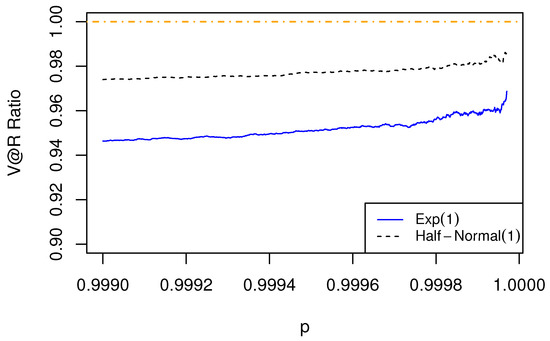
Figure 1. The ratio of $\mathrm{V}@{\mathrm{R}}_p$ of aggregated risk to the sum of $\mathrm{V}@{\mathrm{R}}_p$ of individual risks is less than 1. The dependence structure is specified by a Gumbel–Hougaard copula with the marginal risks being Gumbel.

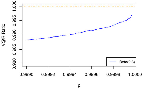
Figure 2. The ratio of $\mathrm{V}@{\mathrm{R}}_p$ of aggregated risk to the sum of $\mathrm{V}@{\mathrm{R}}_p$ of individual risks is less than 1. The dependence structure is specified by a Gumbel–Hougaard copula with the marginal risks being Weibull.

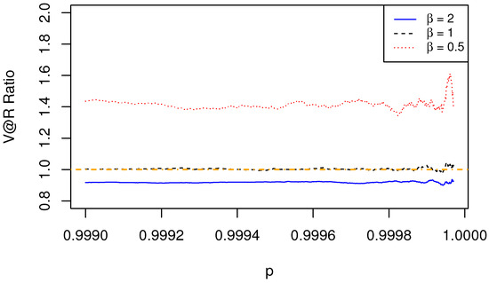
Figure 3. The ratio of $\mathrm{V}@{\mathrm{R}}_p$ of aggregated risk to the sum of $\mathrm{V}@{\mathrm{R}}_p$ of individual risks depends on the value of $\beta$. The dependence structure is specified by a Gumbel–Hougaard copula, with the marginal risks being Fréchet with parameter $\beta$.

One desirable characteristic of the Gumbel–Hougaard copula is that it can be extended to a dependence structure of a higher dimension. Here, we study the numerical results on the three-dimensional case using the Gumbel–Hougaard copula and test the effect of the dependence on the asymptotic additivity of $\mathrm{V}@\mathrm{R}$ for risks in the three MDAs. For the trivariate case, the Gumbel–Hougaard copula has the following form:

$$C\left(u_1,u_2,u_3;\alpha \right)=exp\left[-{\left({\left(-ln{u}_1\right)}^{\alpha }+{\left(-ln{u}_2\right)}^{\alpha }+{\left(-ln{u}_3\right)}^{\alpha }\right)}^{1/\alpha }\right],0\le u_1,u_2,u_3\le 1,$$

where $\alpha \ge 1$. We consider the Gumbel–Hougaard copulas with parameter $\alpha$ equal to 1, 2, 3 and 4.

We have similar observations on all the three MDAs in the trivariate cases as those we have obtained in the bivariate cases. In Figure 4 and Figure 5, we observe that the $\mathrm{V}@\mathrm{R}$ ratios are less than 1. In Figure 6, the results show that whether $\mathrm{V}@\mathrm{R}$ is asymptotic sub/superadditive depends on the value of the Fréchet parameter, $\beta$. $\mathrm{V}@\mathrm{R}$ is asymptotic subadditive for risks with a finite mean and asymptotic superadditive for risks with an infinite mean. In addition, for all the risks, the $\mathrm{V}@\mathrm{R}$ ratios exhibit a tendency to be closer to 1 when $\alpha$ increases. This is because $\mathrm{V}@\mathrm{R}$ is additive when the risks are comonotonoic ($\alpha =\infty$), and in that case the $\mathrm{V}@\mathrm{R}$ ratio equals 1. In general, we observe that the effect of diversification diminishes, which is demonstrated by an increasing $\mathrm{V}@\mathrm{R}$ ratio when the risks are more positively associated. We have shown that it is true for risks with a finite mean but not for risks with an infinite mean. As shown in Figure 6, for Fréchet risk with parameter $\beta =0.5$, the $\mathrm{V}@\mathrm{R}$ ratio is highest when $\alpha =1$, which refers to the case that the risks are independent, and they have the lowest level of association. This is counter-intuitive but consistent with our results in Theorem 4.

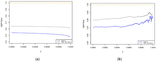
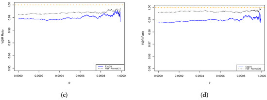
Figure 4. The ratio of $\mathrm{V}@{\mathrm{R}}_p$ of aggregated risk to the sum of $\mathrm{V}@{\mathrm{R}}_p$ of individual risks exhibits a tendency to increase with $\alpha$. The dependence structure is specified by a Gumbel–Hougaard copula of different parameters, with the marginal risks being Gumbel. (a) Gumbel–Hougaard copula parameter $\alpha =1$; (b) Gumbel–Hougaard copula parameter $\alpha =2$; (c) Gumbel–Hougaard copula parameter $\alpha =3$; (d) Gumbel–Hougaard copula parameter $\alpha =4$.

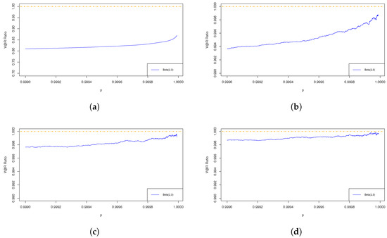
Figure 5. The ratio of $\mathrm{V}@{\mathrm{R}}_p$ of aggregated risk to the sum of $\mathrm{V}@{\mathrm{R}}_p$ of individual risks exhibits a tendency to increase with $\alpha$. The dependence structure is specified by a Gumbel–Hougaard copula of different parameters, with the marginal risks being Weibull. (a) Gumbel–Hougaard copula parameter $\alpha =1$; (b) Gumbel–Hougaard copula parameter $\alpha =2$; (c) Gumbel–Hougaard copula parameter $\alpha =3$; (d) Gumbel–Hougaard copula parameter $\alpha =4$.

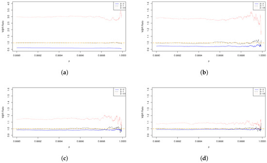
Figure 6. The ratio of $\mathrm{V}@{\mathrm{R}}_p$ of aggregated risk to the sum of $\mathrm{V}@{\mathrm{R}}_p$ of individual risks exhibits a tendency to be closer to 1 when $\alpha$ increases. The dependence structure is specified by a Gumbel–Hougaard copula of different parameters, with the marginal risks being Fréchet with parameter $\beta$ where the red, the black, and the blue curves represent the case of $\beta =0.5,1,$ and 2, respectively. (a) Gumbel–Hougaard copula parameter $\alpha =1$; (b) Gumbel–Hougaard copula parameter $\alpha =2$; (c) Gumbel–Hougaard copula parameter $\alpha =3$; (d) Gumbel–Hougaard copula parameter $\alpha =4$.

4.2. Hüsler–Reiss Copula

The Hüsler–Reiss copula is another extreme-value copula. In the bivariate case, it is defined as

$$C(u_1,u_2;\alpha )=exp\left(-{\widehat{u}}_1\Phi \left[\frac{1}{\alpha }+\frac{\alpha }{2}ln\left(\frac{{\widehat{u}}_1}{{\widehat{u}}_2}\right)\right]-{\widehat{u}}_2\Phi \left[\frac{1}{\alpha }+\frac{\alpha }{2}ln\left(\frac{{\widehat{u}}_2}{{\widehat{u}}_1}\right)\right]\right),0\le u_1,u_2\le 1,$$

where ${\widehat{u}}_1=-ln{u}_1$, ${\widehat{u}}_2=-ln{u}_2$, $\Phi (·)$ is the standard normal distribution function, and $\alpha \in (0,\infty )$. It refers to the case of independence when $\alpha$ approaches 0 and to the case of complete dependence when $\alpha$ approaches infinity. We set $\alpha =1$ in the simulations. Again, Figure 7, Figure 8 and Figure 9 verify our results in Theorems 2–4.

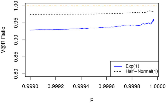
Figure 7. The ratio of $\mathrm{V}@{\mathrm{R}}_p$ of aggregated risk to the sum of $\mathrm{V}@{\mathrm{R}}_p$ of individual risks is less than 1. The dependence structure is specified by a Hüsler–Reiss copula, with the marginal risks being Gumbel.

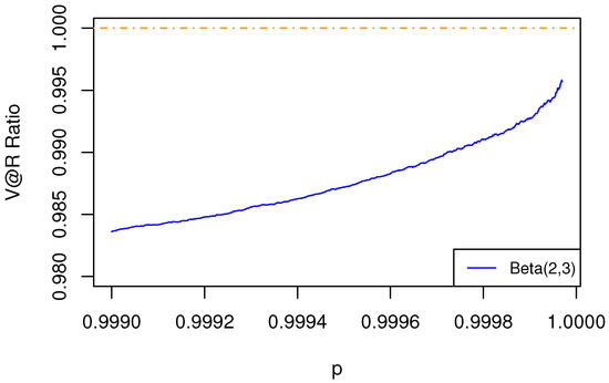
Figure 8. The ratio of $\mathrm{V}@{\mathrm{R}}_p$ of aggregated risk to the sum of $\mathrm{V}@{\mathrm{R}}_p$ of individual risks is less than 1. The dependence structure is specified by a Hüsler–Reiss copula, with the marginal risks being Weibull.

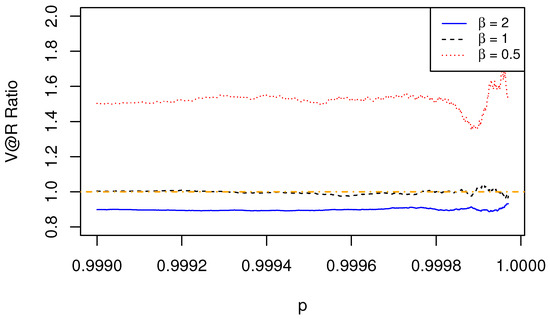
Figure 9. The ratio of $\mathrm{V}@{\mathrm{R}}_p$ of aggregated risk to the sum of $\mathrm{V}@{\mathrm{R}}_p$ of individual risks depends on the value of $\beta$. The dependence structure is specified by a Hüsler–Reiss copula, with the marginal risks being Fréchet.

4.3. The t-EV Copula

The t-EV copula is also an extreme-value copula. The name t-EV comes from Demarta and McNeil (2005), where the bivariate t-EV copula is derived; the multivariate t-EV copula is derived in Nikoloulopoulos et al. (2009).

Let $T_{\nu }$ be the cumulative distribution function of the univariate t-distribution with degree of freedom $\nu >0$. For the bivariate case, with the correlation coefficient $\rho ={\rho }_{12}\in [-1,1]$ and the degree of freedom $\nu$, the copula is defined as

$$C(u_1,u_2;\rho ,\nu )=exp\left[ln\left(u_1{u}_2\right)B(ln{u}_1/ln\left(u_1{u}_2\right);\rho ,\nu )\right],\mathrm{for}0\le u_1,u_2\le 1,$$

where

$$\begin{array}{ccc}\hfill B(w;\rho ,\nu )& =& w{T}_{\nu +1}\left(\frac{\sqrt{\nu +1}}{\sqrt{1-{\rho }^2}}\left[{\left(\frac{w}{1-w}\right)}^{1/\nu }-\rho \right]\right)\hfill \\ & & +(1-w)T_{\nu +1}\left(\frac{\sqrt{\nu +1}}{\sqrt{1-{\rho }^2}}\left[{\left(\frac{1-w}{w}\right)}^{1/\nu }-\rho \right]\right).\hfill \end{array}$$

We set $\rho =0.8$ and $\nu =4$, and obtained the results in Figure 10, Figure 11 and Figure 12, which again verify our main results.

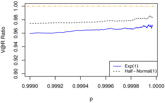
Figure 10. The ratio of $\mathrm{V}@{\mathrm{R}}_p$ of aggregated risk to the sum of $\mathrm{V}@{\mathrm{R}}_p$ of individual risks is less than 1. The dependence structure is specified by a t-EV copula, with the marginal risks being Gumbel.

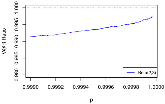
Figure 11. The ratio of $\mathrm{V}@{\mathrm{R}}_p$ of aggregated risk to the sum of $\mathrm{V}@{\mathrm{R}}_p$ of individual risks is less than 1. The dependence structure is specified by a t-EV copula, with the marginal risks being Weibull.

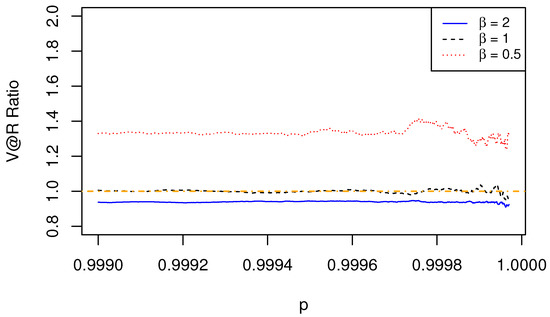
Figure 12. The ratio of $\mathrm{V}@{\mathrm{R}}_p$ of aggregated risk to the sum of $\mathrm{V}@{\mathrm{R}}_p$ of individual risks depends on the value of $\beta$. The dependence structure is specified by a t-EV copula, with the marginal risks being Fréchet.

In addition, the figures for the three extreme-value copula examples show a similar pattern and comparable values in all Gumbel, Weibull, and Fréchet cases. This gives a clue to support that the tail distribution of the common marginal distribution of random variables has a stronger effect than their dependence structure on the tail behaviour of their sum, which echoes and supplements the work of Embrechts et al. (2009b) for extreme-value copulas.

5. Conclusions

In this paper, we have shown the asymptotic sub/super-additivity of $\mathrm{V}@\mathrm{R}$ under extreme-value copulas when the marginal risks are identically distributed and belong to one of the three MDAs of the extreme value distribution. $\mathrm{V}@\mathrm{R}$ is asymptotic subadditive for risks with finite mean. Typically, the insurable risks are considered to have a finite mean so that insurance can be offered profitably with a finite premium. The result echoes the existing works in this area which show that the sub/super-additivity of $\mathrm{V}@\mathrm{R}$ highly depends on the nature of risks (see, for example, Alink et al. 2004 and Embrechts et al. 2009b). It also justifies the standard formula used in Solvency II, where the effect of diversification is introduced by the imperfect correlations between various risk categories. $\mathrm{V}@\mathrm{R}$ is asymptotic superadditive when the risks have a very heavy tail with Fréchet parameter less than 1. This means the pooling of risks cannot reduce the risk exposure. Extremely heavy-tailed risk is now catching the attention of the experts in the field of risk management. For example, Cui et al. (2021) studied the benefit of diversification for insurance of catastrophic risks with limited liability. The development of risk management tools and concepts is essential for the well-being of the society and the financial security of different industries, especially the general insurance industry. Our proofs can be extended to identify a bound for the $\mathrm{V}@\mathrm{R}$ ratio of risks in the MDA of the Fréchet. The bound also depends on the value of Fréchet parameter. It provides us with another angle to understand the nature of the aggregated risk.

References

- Alink, Stan, Matthias Löwe, and Mario Wüthrich. 2004. Diversification of aggregate dependent risks. Insurance: Mathematics and Economics 35: 77–95. [Google Scholar] [CrossRef]
- Alm, Jonas. 2016. Signs of dependence and heavy tails in non-life insurance data. Scandinavian Actuarial Journal 2016: 859–75. [Google Scholar] [CrossRef]
- Asimit, Alexandru, and Bruce Jones. 2007. Extreme behavior of bivariate elliptical distributions. Insurance: Mathematics and Economics 41: 53–61. [Google Scholar] [CrossRef]
- Asimit, Alexandru, Edward Furman, Qihe Tang, and Raluca Vernic. 2011. Asymptotics for risk capital allocations based on conditional tail expectation. Insurance: Mathematics and Economics 49: 310–24. [Google Scholar] [CrossRef]
- Barbe, Philippe, Anne-Laure Fougères, and Christian Genest. 2006. On the tail behavior of sums of dependent risks. ASTIN Bulletin: The Journal of the IAA 36: 361–73. [Google Scholar] [CrossRef]
- Bäuerle, Nicole, and Alfred Müller. 1998. Modeling and comparing dependencies in multivariate risk portfolios. ASTIN Bulletin: The Journal of the IAA 28: 59–76. [Google Scholar] [CrossRef]
- Beirlant, Jan, Yuri Goegebeur, Johan Segers, and Jozef Teugels. 2006. Statistics of Extremes: Theory and Applications. Hoboken: John Wiley & Sons. [Google Scholar]
- Cherubini, Umberto, Sabrina Mulinacci, Fabio Gobbi, and Silvia Romagnoli. 2011. Dynamic Copula Methods in Finance. Hoboken: John Wiley & Sons. [Google Scholar]
- Cheung, Ka Chun, Hok Kan Ling, Qihe Tang, Sheung Chi Phillip Yam, and Fei Lung Yuen. 2019. On additivity of tail comonotonic risks. Scandinavian Actuarial Journal 2019: 837–66. [Google Scholar] [CrossRef]
- Cui, Hengxin, Ken Seng Tan, and Fan Yang. 2021. Diversification in Catastrophe Insurance Markets. ASTIN Bulletin 51: 753–78. [Google Scholar] [CrossRef]
- de Haan, Laurens, and Ana Ferreira. 1999. Extreme Value Theory: An Introduction. New York: Springer. [Google Scholar]
- de Haan, Laurens, and Sidney Resnick. 1977. Limit theory for multivariate sample extremes. Zeitschrift für Wahrscheinlichkeitstheorie und verwandte Gebiete 40: 317–37. [Google Scholar] [CrossRef]
- Deheuvels, Paul. 1984. Probabilistic aspects of multivariate extremes. In Statistical Extremes and Applications. Dordrecht: Springer, pp. 117–30. [Google Scholar]
- Demarta, Stefano, and Alexander McNeil. 2005. The t copula and related copulas. International Statistical Review 73: 111–29. [Google Scholar] [CrossRef]
- Denuit, Michel, Jan Dhaene, Marc Goovaerts, and Rob Kaas. 2005. Actuarial Theory for Dependent Risks: Measures, Orders and Models. Hoboken: John Wiley & Sons, Ltd. [Google Scholar]
- Embrechts, Paul. 2000. Extreme value theory: Potential and limitations as an integrated risk management tool. Derivatives Use, Trading & Regulation 6: 449–56. [Google Scholar]
- Embrechts, Paul, Claudia Klüppelberg, and Thomas Mikosch. 2013. Modelling Extremal Events: For Insurance and Finance. Cham: Springer Science & Business Media, vol. 33. [Google Scholar]
- Embrechts, Paul, Dominik Lambrigger, and Mario Wüthrich. 2009a. Multivariate extremes and the aggregation of dependent risks: Examples and counter-examples. Extremes 12: 107–27. [Google Scholar] [CrossRef]
- Embrechts, Paul, Johanna Nešlehová, and Mario Wüthrich. 2009b. Additivity properties for Value-at-Risk under Archimedean dependence and heavy-tailedness. Insurance: Mathematics and Economics 44: 164–69. [Google Scholar] [CrossRef]
- Falk, Michael, Jürg Hüsler, and Rolf-Dieter Reiss. 2010. Laws of Small Numbers: Extremes and Rare Events. Cham: Springer Science & Business Media. [Google Scholar]
- Frees, Edward, and Emiliano Valdez. 1998. Understanding relationships using copulas. North American Actuarial Journal 2: 1–25. [Google Scholar] [CrossRef]
- Frey, Rüdiger, and Alexander McNeil. 2001. Modelling Dependent Defaults. Unpublished working paper. Zurich: ETH Zurich. [Google Scholar]
- Galambos, Janos. 1975. Order statistics of samples from multivariate distributions. Journal of the American Statistical Association 70: 674–80. [Google Scholar]
- Galambos, Janos. 1978. The Asymptotic Theory of Extreme Order Statistics. Wiley Series in Probability and Mathematical Statistics. New York, Chichester and Brisbane: John Wiley & Sons. [Google Scholar]
- Genest, Christian, and Louis-Paul Rivest. 1989. A characterization of Gumbel’s family of extreme value distributions. Statistics & Probability Letters 8: 207–11. [Google Scholar]
- Gudendorf, Gordon, and Johan Segers. 2010. Extreme-value Copulas. In Copula Theory and Its Applications. Berlin and Heidelberg: Springer, pp. 127–45. [Google Scholar]
- Gudendorf, Gordon, and Johan Segers. 2012. Nonparametric estimation of multivariate extreme-value copulas. Journal of Statistical Planning and Inference 142: 3073–85. [Google Scholar] [CrossRef]
- Hall, Peter, and Nader Tajvidi. 2000. Distribution and dependence-function estimation for bivariate extreme-value distributions. Bernoulli 6: 835–44. [Google Scholar] [CrossRef]
- Hua, Lei. 2017. On a bivariate copula with both upper and lower full-range tail dependence. Insurance: Mathematics and Economics 73: 94–104. [Google Scholar] [CrossRef]
- Hua, Lei, and Harry Joe. 2012. Tail comonotonicity: Properties, constructions, and asymptotic additivity of risk measures. Insurance: Mathematics and Economics 51: 492–503. [Google Scholar] [CrossRef]
- Joe, Harry. 1997. Multivariate Models and Dependence Concepts. Volume 73 of Monographs on Statistics and Applied Probability. London: Chapman & Hall. [Google Scholar]
- Joe, Harry. 2014. Dependence Modeling with Copulas. London: Chapman & Hall. [Google Scholar]
- Kotz, Samuel, and Saralees Nadarajah. 2000. Extreme Value Distributions: Theory and Applications. Singapore: World Scientific. [Google Scholar]
- Kremer, Erhard. 1998. Largest claims reinsurance premiums under possible claims dependence. ASTIN Bulletin: The Journal of the IAA 28: 257–67. [Google Scholar] [CrossRef]
- Li, Haijun. 2013. Toward a Copula Theory for Multivariate Regular Variation. In Copulae in Mathematical and Quantitative Finance. Edited by Piotr Jaworski, Fabrizio Durante and Wolfgang Härdle. Lecture Notes in Statistics. Berlin/Heidelberg: Springer, vol. 213. [Google Scholar]
- McNeil, Alexander, Rüdiger Frey, and Paul Embrechts. 2005. Quantitative Risk Management: Concepts, Techniques and Tools. Princeton Series in Finance. Princeton: Princeton University Press. [Google Scholar]
- Nelsen, Roger. 2006. An Introduction to Copulas. Cham: Springer Science & Business Media. [Google Scholar]
- Nikoloulopoulos, Aristidis, Harry Joe, and Haijun Li. 2009. Extreme value properties of multivariate t copulas. Extremes 12: 129–148. [Google Scholar] [CrossRef]
- Pfeifer, Dietmar, and Doreen Strassburger. 2008. Solvency II: Stability Problems with the SCR Aggregation Formula. Scandinavian Actuarial Journal 2008: 61–77. [Google Scholar] [CrossRef]
- Pfeifer, Dietmar, and Olena Ragulina. 2018. Generating VaR Scenarios under Solvency II with Product Beta Distributions. Risks 6: 122. [Google Scholar] [CrossRef]
- Pfeifer, Dietmar, and Olena Ragulina. 2021. Generating unfavourable VaR scenarios under Solvency II with patchwork copulas. Dependence Modeling 9: 327–46. [Google Scholar] [CrossRef]
- Pickands, James. 1981. Multivariate extreme value distributions. Paper presented at 43rd Session of the International Statistical Institute (Buenos Aires), Buenos Aire, Argentina, November 30–December 11; pp. 859–78. [Google Scholar]
- Poon, Ser-Huang, Michael Rockinger, and Jonathan Tawn. 2004. Extreme value dependence in financial markets: Diagnostics, models, and financial implications. The Review of Financial Studies 17: 581–610. [Google Scholar] [CrossRef]
- Resnick, Sidney. 2013. Extreme Values, Regular Variation and Point Processes. Cham: Springer. [Google Scholar]
- Sandström, Arne. 2007. Solvency II: Calibration for skewness. Scandinavian Actuarial Journal 2007: 126–34. [Google Scholar] [CrossRef]
- Su, Jianxi, and Lei Hua. 2017. A general approach to full-range tail dependence copulas. Insurance: Mathematics and Economics 77: 49–64. [Google Scholar] [CrossRef]
- Vesa, Ronkainen, Koskinen Lasse, and Berglund Raoul. 2007. Topical modelling issues in Solvency II. Scandinavian Actuarial Journal 2007: 135–46. [Google Scholar] [CrossRef]
Disclaimer/Publisher’s Note: The statements, opinions and data contained in all publications are solely those of the individual author(s) and contributor(s) and not of MDPI and/or the editor(s). MDPI and/or the editor(s) disclaim responsibility for any injury to people or property resulting from any ideas, methods, instructions or products referred to in the content. |
© 2023 by the authors. Licensee MDPI, Basel, Switzerland. This article is an open access article distributed under the terms and conditions of the Creative Commons Attribution (CC BY) license (https://creativecommons.org/licenses/by/4.0/).