Robust Classification via Support Vector Machines

Abstract

Classification models are very sensitive to data uncertainty, and finding robust classifiers that are less sensitive to data uncertainty has raised great interest in the machine learning literature. This paper aims to construct robust support vector machine classifiers under feature data uncertainty via two probabilistic arguments. The first classifier, Single Perturbation, reduces the local effect of data uncertainty with respect to one given feature and acts as a local test that could confirm or refute the presence of significant data uncertainty for that particular feature. The second classifier, Extreme Empirical Loss, aims to reduce the aggregate effect of data uncertainty with respect to all features, which is possible via a trade-off between the number of prediction model violations and the size of these violations. Both methodologies are computationally efficient and our extensive numerical investigation highlights the advantages and possible limitations of the two robust classifiers on synthetic and real-life insurance claims and mortgage lending data, but also the fairness of an automatized decision based on our classifier.

1. Introduction

Binary classification is a standard prediction model in machine learning and statistical learning that aims to predict whether a randomly chosen data point belongs to one of two possible classes. There is a wider range of applications, but detecting insurance fraud and predicting mortgage-lending decisions are the most common applications of binary classification in the insurance and financial sectors. Motor insurance is massively affected by fraud, especially for a third-party liability line of business that is often not profitable, and, thus, reducing the fraud insurance has obvious financial incentives. At the same time, an effective fraud detection model would also help to reduce the unintended discriminatory effects observed in the insurance supply for potential policyholders from certain locations and/or having some particular characteristics related to race and ethnicity; this effect is known in the insurance literature as redlining. The decisions with respect to mortgage lending (but also other non-mortgage products affected by credit risk, e.g., applicants for credit cards, auto loans, student loans, etc.) are very sensitive decisions that require a balance between a low prediction error and reducing the effect of the unintended discriminatory effects of such decisions. The literature on these two applications is quite rich, e.g., see Bermudez et al. (2008) and Artis et al. (1999) for insurance fraud detection, and Kallus et al. (2022), Zhang (2016) and Steenackers and Goovaerts (1989) for predicting mortgage-lending decisions and evaluating the fairness of such decisions.

A prediction model is said to be robust if small changes in the data would not change the model outputs, which is a consistent interpretation of robust prediction modeling across the theoretical statistics and computational robustness literature. Standard practical approaches to achieve robust predictions in the machine learning literature include outlier detection, testing prediction performance under data contamination or allowing for data uncertainty (DU) in the prediction model.

Creating robust prediction models is imperative whenever the current and/or future data are affected by DU. Specifically, DU means that the data are affected by (i) the sampling error, (ii) ambiguity or (iii) data noise, and each source of DU affects the robustness of the prediction model. The sampling error is inevitable, and this source of DU is negligible in large samples, which is often the case in machine learning modeling. Data ambiguity goes beyond missing data, and is a challenging issue that often occurs in categorical data. For example, insurance fraud data contain information about the event leading to a claim (major/minor) that is very subjective; similarly, Likert scale features in automatized hiring processes are influenced by ambiguous questionnaires. Data noise is the unexplained variability within the observational data. The data noise could be associated with the features or response variable(s) in supervised learning. In summary, data ambiguity and feature and/or label noise are the important sources of DU, though data noise is the main source of DU considered in the robust classification literature.

A support vector machine (SVM) is an effective classifier with a variety of real-world applications due to its simplicity, and, thus, is one of the most important (distance-based) classification methods in the machine learning and statistical learning literature. However, the SVM is very sensitive to label and feature noise, and, thus, a large amount of work has been carried out to robustify SVMs against such sources of DU. For example, prior studies dealing with various loss functions have been used to robustify SVM predictions with respect to feature noise (Bamakan et al. 2017; Shen et al. 2017; Singh et al. 2014; Suykens and Vandewalle 1999); standard approaches have also been explored in the field of robust optimization (RO), such as metric-type (non-probabilistic) uncertainty sets (Bertsimas et al. 2018; Bi and Zhang 2005); another RO approach, namely, chance constraints (CC), which are probabilistic uncertainty sets, has been introduced in the literature so that the underlying optimization problems used in SVM prediction exhibit more robust outputs whenever DU is present (Huang et al. 2012; Lanckriet et al. 2002).

The main purpose of this paper is to reduce the effect of feature noise for binary SVM classifiers. We explore the internal structure of the classical SVM (C-SVM) classifier in order to detect and tackle the feature noise via probabilistic arguments, while the eventual label noise issue is put aside in this paper, since our proposed probabilistic arguments are not easily extendable to prediction modeling under label noise.

The first proposed robust SVM classifier is the Single Perturbation (SP-SVM), and aims to reduce the local effect of DU with respect to one given feature by embedding this possible source of uncertainty into the prediction model. This technique is very popular in RO, where the so-called CCs are constructed to replace its non-robust counterparts (that are assumed to be certain). SP-SVM is an effective classifier whenever DU is present, and it could be used to test whether or not each feature is affected by DU.

The second proposed robust SVM classifier is the Extreme Empirical Loss (EEL-SVM), and aims to reduce the aggregate effect of DU. This is achieved by introducing a trade-off between the number of prediction model violations (misclassifications) and the size of these violations, which is explained via a probabilistic argument. Simply speaking, C-SVM assigns the same importance (probability) to each misclassification and aims to reduce the overall prediction error. In contrast, EEL-SVM focuses only on the most significant errors, i.e., the extreme errors, which increases the accuracy around the borderline decisions and improves the model accuracy. This approach is inspired by the standard risk measure, namely, conditional value-at-risk, which was shown to be very robust in the context of model ambiguity modeled via RO (Asimit et al. 2017).

C-SVM is a special case of both SP-SVM and EEL-SVM, and, thus, our robust formulations generalize C-SVM. Efficient convex quadratic programming solvers are used for solving SP-SVM and EEL-SVM, but the computational times of SP-SVM and EEL-SVM are not smaller than C-SVM, and this effect is known in the RO literature as the price of robustness. Note that, due to its sparsity, EEL-SVM has a lower computational time than SP-SVM and the reduction in computational time is mainly influenced by the sample size. Our numerical experiments have shown that both SP-SVM and EEL-SVM perform very well when compared with their robust SVM competitors. Moreover, even though the overall performance of SP-SVM is slightly superior to EEL-SVM, the sparsity trait of EEL-SVM is extremely appealing from a computational perspective; for specific details about our numerical experiments, see Section 4.

It is worth noting that, unlike the existing methods based on CC  (Lanckriet et al. 2002; Wang et al. 2018), SP-SVM does not require estimating the covariance matrix, which is not always computationally stable  (Fan et al. 2016; Ledoit and Wolf 2020). Moreover, in this paper, we only provide explicit derivations for SP-SVM and EEL-SVM with the most popular loss function, i.e., hinge loss, but similar derivations are possible for any other loss function. In addition to the two new robust SVM models, we also prove Fisher consistency for a general convex loss function and binary SVM classifier.

The paper is organized as follows. Section 2 provides the necessary background, while Section 3 illustrates the two proposed robust SVM classifiers. Section 4 summarizes our numerical experiments conducted over synthetic and real-life datasets. All proofs are relegated to the Appendix A.

2. Background and Problem Definition

The current section takes stock of the necessary background related to binary SVM classification. Section 2.1 briefly explains the C-SVM formulation, while Section 2.2 provides a comprehensive description of the pros and cons of various loss functions, which is a pivotal choice for any SVM implementation. Finally, Section 2.3 discusses the importance of the Fisher consistency property in classification followed by a theoretical contribution in the context of binary classification, which is stated as Theorem 1.

2.1. Problem Definition

Our starting point is the training set that contains N instances and their associated labels, $\{({\mathbf{x}}_i,y_i),i=1,\dots ,N\}$, where ${\mathbf{x}}_i\in \mathcal{X}\subseteq {\mathbb{R}}^d$ and $y_i\in \mathcal{Y}$. The training set is assumed to be sampled from $(X,Y)$, but the binary classification reduces to $\mathcal{Y}:=\{-1,1\}$, where $y_i=1$ if ${\mathbf{x}}_i$ is in the positive class, ${\mathcal{C}}_{+1}$, and $y_i=-1$ if ${\mathbf{x}}_i$ is in the negative class, ${\mathcal{C}}_{-1}$. The main objective is to construct an accurate (binary) classifier $c:\mathcal{X}\to \mathcal{Y}$ that maximizes the probability that $c\left({\mathbf{x}}_i\right)=y_i$.

SVM aims to identify a separation hyper-plane ${\mathbf{w}}^T\varphi \left(\mathbf{x}\right)+b$ that generates two parallel supporting hyper-planes:

$${\mathbf{w}}^T\varphi \left(\mathbf{x}\right)+b=1\mathrm{and}{\mathbf{w}}^T\varphi \left(\mathbf{x}\right)+b=-1,$$

(1)

where $\varphi (·)$ is a notional function that transforms the feature space into a synthetic feature space that allows for a linear hyper-plane separation of the data (when linear classifiers are not effective on the original data). The data are rarely perfectly separable, and a compromise is made by allowing classification violations for the non-separable data. The latter is also known as soft-margin SVM and is formulated as follows:

$${\displaystyle \underset{\mathbf{w},b}{\min }\frac{1}{2}{\mathbf{w}}^T\mathbf{w}+C\sum _{i=1}^{N}L(1-y_i({\mathbf{w}}^T\varphi \left({\mathbf{x}}_i\right)+b)).}$$

(2)

The first term aims to find the ‘best’ classifier by maximizing the distance between the two hyper-planes defined in (1), whereas the second term penalizes the classifier’s violations measured via a given loss function $L:\mathbb{R}\to {\mathbb{R}}_{+}$; for details, see Vapnik (2000).

2.2. Loss Function

Solving the general SVM formulation in (2) requires specific solvers that depend upon the loss function choice, which has a central role in SVM classification. The existing literature has dealt with numerous piecewise loss functions, and a summary is given below:

(i)

Hinge loss:$L_H\left(u\right):=max\{0,u\}$;

(ii)

Truncated hinge loss ($a\ge 1$):$L_{TH}\left(u\right):=min\{max\{0,u\},a\}$;

(iii)

Pinball loss ($a\le 0$):$L_P\left(u\right):=max\{au,u\}$;

(iv)

Pinball loss with ‘ϵ zone’ ($ϵ\ge 0$ and $a,b\le 0$):$L_{PEZ}\left(u\right):=max\{0,u-ϵ,au+b\}$;

(v)

Truncated pinball loss ($a\le 0$ and $b\ge 0$):$L_{TP}\left(u\right):=max\{u,min\{au,b\}\}$.

The standard choice, $L_H$, leads to efficient computations as it reduces (2) to solving a convex linearly constrained quadratic program (LCQP), which is the original SVM formulation as explained in Vapnik (2000). Moreover, the hinge loss is proved to be an upper bound of the classification error (Shen et al. 2017; Zhang 2004); therefore, it is a pivotal loss choice. At the same time, the hinge loss has been criticized for not being robust and extremely sensitive to outliers, whereas the truncated hinge loss proposed by Wu and Liu (2007) overcomes this issue at the expense of computational complexity. The lack of convexity of this loss function requires a bespoke algorithm, namely, the difference of convex functions optimization algorithm (DCA), which is computationally less efficient than standard LCQP solvers used for solving C-SVM and our proposed robust formulations (SP-SVM and EEL-SVM). The optimization problems based on the two pinball losses require solving LCQPs with many more linear equality constraints than the hinge loss, but the pinball loss seems to be more robust and stable when re-sampling (Huang et al. 2014). Similar arguments have been used in Shen et al. (2017) to justify that the truncated pinball loss is a good choice when dealing with feature noise, though it shares the same computational shortcoming as the truncated hinge loss: it requires non-convex solvers.

All previous five loss functions are piecewise linear, which is a computational advantage, but non-piecewise linear loss functions have been proposed in the existing literature. For example, the least square loss with $L_{LS}\left(u\right):=u^2$ is considered in Suykens and Vandewalle (1999), for which, an efficient LCQP formulation is proposed; the correntropy loss is defined in Singh et al. (2014), but variants of this have been investigated (see Xu et al. 2017 for SVM-like formulations). One could understand the possible advantages of non-linear convex loss functions for other classification methods from Lin (2004), where the hinge loss is shown to be the tightest margin-based upper bound of the misclassification loss for many well-known classifiers. Further, it is numerically shown that this property does not justify thinking of the hinge loss as the universally ‘best’ choice to measure misclassification. Strictly convex loss functions are argued in Bartlett et al. (2006) to possess appealing statistical properties when studying misclassification.

Even though the loss function is a pivotal choice in SVM classification, our two new robust classifiers are not restricted to a specific loss function, and, thus, SP-SVM and EEL-SVM formulations are quite general and introduce two new methodologies of tackling binary classification in the presence of DU. However, the SP-SVM (instance (6)) and EEL-SVM (instance (11)) illustrations of this paper are only focused on hinge loss formulations, though any other illustrations are possible. Therefore, the robustness of SP-SVM and EEL-SVM is a result of how these classifiers deal with DU, and not a by-product of choosing the ‘best’ loss function.

2.3. Fisher Consistency

A desirable loss function property for a generic classifier is Fisher consistency or classification calibration (Bartlett et al. 2006). By definition, the loss function L is Fisher consistent if

$$\underset{f:\mathcal{X}\to \mathbb{R}}{arg\; min}{\mathbf{E}}_{\mathcal{X},\mathcal{Y}}L\left(1-Yf\left(\mathbf{X}\right)\right)$$

(3)

is solved by the Bayes classifier that is defined as follows:

$$f_{Bayes}^{*}\left(\mathbf{x}\right)=\left\{\begin{array}{ccc}\hfill 1,& \mathrm{if}\hfill & Pr(Y=1|\mathbf{x})>Pr(Y=-1\left|\mathbf{x}\right),\hfill \\ \hfill -1,& \mathrm{if}\hfill & Pr(Y=1|\mathbf{x})<Pr(Y=-1\left|\mathbf{x}\right).\hfill \end{array}\right.$$

In the context of binary SVM classification, one could show that (3) holds if

$$\begin{array}{c}\hfill \underset{z\in \mathbb{R}}{arg\; min}{\mathbf{E}}_{\mathcal{Y}|\mathbf{x}}L(1-Yz)=f_{Bayes}^{*}\left(\mathbf{x}\right)\end{array}$$

(4)

is true for all $\mathbf{x}\in \mathcal{X}$; e.g., see Proposition 1 in Wu and Liu (2007).

Fisher consistency has been extensively investigated in the literature, and we now provide a concise review that relates to our framework. Theorem 3.1 in Lin (2004) shows that, if the global minimizer of (3) exists, then it has to be the same as the Bayes decision rule, which is valid for any classification method. In the binary SVM setting, Proposition 1 in Wu and Liu (2007) and Theorem 1 in Shen et al. (2017) show that this property also holds for non-convex loss functions; the first result covers a large set of truncated loss functions, whereas the second focuses on the truncated pinball loss. Lemma 3.1 of Lin (2002) shows that the hinge loss is Fisher consistent, and Theorem 1 in Huang et al. (2014) shows the same for the (convex loss) pinball loss. Our next result extends Fisher consistency to a general convex loss function L for the binary SVM case, and its proof is relegated to Appendix A.1.

Theorem 1.

Assume that $L:\mathbb{R}\to {\mathbb{R}}_{+}$ is a convex loss function that vanishes at 0, i.e., $L\left(0\right)=0$. If $L(·)$ is linear in $(0,2+ϵ)$ for some $ϵ>0$, then L is Fisher consistent.

2.4. Related Work

Most robust SVM algorithms for solving the feature noise problem are designed following two approaches. The first approach is to replace the hinge loss function in C-SVM by more robust ones, such as the truncated hinge loss (Wu and Liu 2007), pinball loss (Huang et al. 2014), or truncated pinball loss (Shen et al. 2017). However, as discussed in Section 2.2, these methods are less computationally efficient compared to the proposed SP-SVM and EEL-SVM with standard choice of hinge loss. The second approach, coming from operational research, involves chance constraints to quantify the probability of misclassification for uncertain data. For example,  Lanckriet et al. (2002) propose minimizing the maximum probability of misclassification assuming that the mean and covariance matrix are known. Wang et al. (2018) obtain the equivalent semidefinite programming (SDP) and second-order cone programming (SOCP) models for chance-constrained-SVM (CC-SVM). However, in real applications, the moments are usually unknown and must be estimated from observations. Unfortunately, estimating a large covariance matrix is not always computationally stable (Fan et al. 2016; Ledoit and Wolf 2020). Compared to existing CC-SVM models, SP-SVM can avoid this estimation problem by only focusing on the feature most affected by DU.

3. Robust SVM

This section explains the concept of a robust SVM in a more formal way and provides the technical details for our two robust SVMs; that is, SP-SVM in Section 3.1, and EEL-SVM in Section 3.2. Finally, a summary of practical recommendations when using our robust SVM formulations is given in Section 3.3.

3.1. Single Perturbation SVM

SP-SVM aims to reduce the local effect of DU with respect to one given feature by embedding this possible source of uncertainty into the optimization problem that describes our robust prediction model. The main idea is the appropriation of a standard RO approach that relies on CCs constructed to replace its non-robust counterparts (assumed to hold almost surely). That is, SP-SVM extends C-SVM by adjusting the feasibility set through parameter $\alpha$ that controls the DU level; $\alpha$ is tuned like in any other hyper-parameter model.

Previous robust SVM classifiers that rely on CC require the covariance (feature) matrix estimate, which is computable but brings some practical drawbacks; the empirical covariance matrix is computationally unstable when d is large, and is often not positive semi-definite if missing values are present in the sample. This is not the case for SP-SVM, whose robustness is achieved by identifying the feature affected the most by DU. We choose this feature as the one with the highest variance whenever data are less interpretable (see Section 4.1 and Section 4.2), though domain knowledge could help with choosing this feature (see Section 4.3).

Solving (2) under the hinge loss is equivalent to solving the following LCQP instance:

$$\begin{array}{ccc}& & {\displaystyle \underset{\mathbf{w},b,\xi }{\min }\frac{1}{2}{\mathbf{w}}^T\mathbf{w}+C\sum _{i=1}^N{\xi }_i}\hfill \\ & & \mathrm{s}.\mathrm{t}.y_i\left({\mathbf{w}}^T\varphi \left({\mathbf{x}}_i\right)+b\right)\ge 1-{\xi }_i,{\xi }_i\ge 0,1\le i\le N,\hfill \end{array}$$

(5)

where $C>0$ is a penalty constant that becomes a tuning parameter in the actual implementation phase. Equation (5) represents the mathematical formulation of C-SVM.

We are interested in calibrating (5) in the presence of DU with respect to one feature, e.g., the $k^{th}$ feature. Thus, the $j^{th}$ entry of $\varphi \left({\mathbf{x}}_i\right)$, denoted by ${\varphi }_j\left({\mathbf{x}}_i\right)$, is deterministic for all $1\le i\le N$ and $1\le j\ne k\le d$, whereas the $k^{th}$ feature is affected by an error term $Z_{ik}$; hence, ${\varphi }_k\left({\mathbf{x}}_i\right)$ is replaced by ${\varphi }_k\left({\mathbf{x}}_i\right)+Z_{ik}$ for all $1\le i\le N$. Moreover, each error term is defined on a probability space $({\mathsf{\Omega }}_{ik},\mathcal{F},P)$ with ${\mathsf{\Omega }}_{ik}\subseteq \mathbb{R}$. Therefore, the DU variant of (5) with respect to the $k^{th}$ feature becomes

$$\begin{array}{ccc}& & {\displaystyle \underset{\mathbf{w},b,\xi }{\min }\frac{1}{2}{\mathbf{w}}^T\mathbf{w}+C\sum _{i=1}^N{\xi }_i}\hfill \\ & & \mathrm{s}.\mathrm{t}.Pr\left(y_i\left({\mathbf{w}}^T\varphi \left({\mathbf{x}}_i\right)+w_k{Z}_{ik}+b\right)\ge 1-{\xi }_i\right)\ge \alpha ,{\xi }_i\ge 0,1\le i\le N,\hfill \end{array}$$

(6)

where $\alpha \in [0,1]$ reflects the unknown modeler’s perception of DU that is later tuned. This kind of probability-like constraint is also known as CC in the OR literature.

For any given tuple $(i,k)$, the cumulative distribution function (cdf) of $Z_{ik}$, $F_{ik}(·)$ is defined on ${\mathsf{\Omega }}_{ik}$. Furthermore, we define two generalized inverse functions as follows:

$$F_{ik}^{-1}\left(t\right):=inf\left\{x\in \mathbb{R}:F_{ik}\left(x\right)\ge t\right\}\mathrm{and}{F}_{ik}^{-1+}\left(t\right):=sup\left\{x\in \mathbb{R}:F_{ik}\left(x\right)\le t\right\}$$

for all $t\in [0,1]$, where $inf⌀=\infty$ and $sup⌀=-\infty$ hold by convention. Clearly,

$$t\le Pr\left(Z_{ik}\le x\right)\iff F_{ik}^{-1}\left(t\right)\le x\mathrm{and}Pr\left(Z_{ik}<x\right)\le t\iff x\le F_{ik}^{-1+}\left(t\right),x\in \mathbb{R}\mathrm{and}t\in [0,1].$$

Therefore, the CC from (6) is equivalent to

$$y_i\left({\mathbf{w}}^T\varphi \left({\mathbf{x}}_i\right)+b\right)+y_i{w}_k{F}_{ik}^{-1+}(1-\alpha )\ge 1-{\xi }_i,y_i\left({\mathbf{w}}^T\varphi \left({\mathbf{x}}_i\right)+b\right)+y_i{w}_k{F}_{ik}^{-1}\left(\alpha \right)\ge 1-{\xi }_i$$

(7)

when $y_i{w}_k\ge 0$ or $y_i{w}_k<0$, respectively. Without imposing any restriction on $F_{ik}$, the conditional constraint from (7) makes (6) a mixed integer programming instance, which is a major computational shortcoming for large scale problems. The next set of conditions enable us to solve (6) efficiently.

Assumption 1.

$F_{ik}^{-1}\left(\alpha \right)+F_{ik}^{-1+}(1-\alpha )=0$ for a given integer $1\le k\le d$ and some $\alpha \in [0,1]$.

If the random error $Z_{ik}$ is defined on ${\mathsf{\Omega }}_{ik}=\left(-{\omega }_{ik},{\omega }_{ik}\right)$ with $0<{\omega }_{ik}\le \infty$ such that its cdf is continuous and increasing, and $F_{ik}(·)+F_{ik}(-·)=1$ in a neighborhood of $F_{ik}^{-1+}\left(\alpha \right)$, then Assumption 1 holds. Note that symmetric and continuous cdfs, such as Gaussian, Student’s t or any other member of the elliptical family of distributions centered at 0, satisfy Assumption 1; for details, see Fang et al. (1990). Therefore, Assumption 1 is quite general.

Under Assumption 1, (7) is equivalent to

$$y_i\left({\mathbf{w}}^T\varphi \left({\mathbf{x}}_i\right)+b\right)-\left|w_k\right|F_{ik}^{-1}\left(\alpha \right)\ge 1-{\xi }_i,$$

and, in turn, (6) is equivalent to solving

$$\begin{array}{ccc}\underset{\mathbf{w},b,\xi }{\min }\hfill & {\displaystyle \frac{1}{2}{\mathbf{w}}^T\mathbf{w}+C\sum _{i=1}^N{\xi }_i}\hfill & \\ \mathrm{s}.\mathrm{t}.\hfill & y_i\left({\mathbf{w}}^T\varphi \left({\mathbf{x}}_i\right)+b\right)\ge 1-{\xi }_i\hfill & \left(\mathrm{i}\right)\\ \hfill & y_i\left({\mathbf{w}}^T\varphi \left({\mathbf{x}}_i\right)+b\right)-y_i{w}_k{a}_{ik}\ge 1-{\xi }_i\hfill & \left(\mathrm{ii}\right)\\ \hfill & y_i\left({\mathbf{w}}^T\varphi \left({\mathbf{x}}_i\right)+b\right)+y_i{w}_k{a}_{ik}\ge 1-{\xi }_i\hfill & \left(\mathrm{iii}\right)\\ \hfill & {\xi }_i\ge 0,1\le i\le N,\hfill & \left(\mathrm{iv}\right)\end{array}$$

(8)

where $a_{ik}:=F_{ik}^{-1}\left(\alpha \right)$. If $a_{ik}\le 0$ for all $1\le i\le N$, then the inequality constraints (8) (ii) and (iii) are redundant, and, thus, SP-SVM and SVM are identical, i.e., the $k^{th}$ feature is not affected by DU. If $a_{ik}\ge 0$ for all $1\le i\le N$, then the inequality constraint (8) (i) is redundant and the $k^{th}$ feature is affected by DU, in which case, SP-SVM becomes more conservative than SVM, i.e., the SP-SVM hyper-plane violations ${\xi }_i$s are allowed to be larger (than the C-SVM violations) due to DU.

We now provide a practical recommendation for finding a ‘reasonable’ choice for $a_{ik}$. One possibility is to assume a Gaussian random noise with zero mean and variance equal to the sampling error estimate, i.e.,

$$a_{ik}={\widehat{a}}_k:=q_{\alpha ,G}\sqrt{{\displaystyle \frac{1}{N-1}\sum _{i=1}^N{(x_{ik}-{\overline{x}}_k)}^2}}\mathrm{and}{\overline{x}}_k:=\frac{1}{N}\sum _{i=1}^N{x}_{ik}\mathrm{for}\mathrm{all}1\le i\le N,$$

where $q_{\alpha ,G}$ is the $\alpha$-normal quantile. It could be argued that the Gaussian random noise might underestimate DU; hence, a more heavy-tailed noise, such as Student’s t, might be more appropriate. In that case, we could simply replace $q_{\alpha ,G}$ by the $\alpha$-quantile of the distribution of choice. We always tune $\alpha$ for values greater than $0.5$, i.e., $a_{ik}>0$ for all $1\le i\le N$, since DU is assumed to be present. Therefore, our SP-SVM implementations require solving LCQP instances with $3N$ inequality constraints, though C-SVM implementations require solving LCQP instances with $2N$ inequality constraints; this is not surprising and is known as the price of robustness in the OR literature. An explicit solution for (8) is detailed in Appendix A.2, where we do not make any assumption on the sign of $a_{ik}$’s.

3.2. Extreme Empirical Loss SVM

EEL-SVM is designed to reduce the overall effect of DU with respect to all features that are possibly affected by random noise, which is different from SP-SVM, where only one feature is assumed to be affected by noise. This does not mean that EEL-SVM is ‘better’ than SP-SVM, as the two approaches complement each other, and Section 4 provides empirical evidence in that sense.

Simply speaking, EEL-SVM creates a trade-off between the number of model misclassifications and the size of these violations, which is explained via a probabilistic argument. Whereas C-SVM assigns the same importance (probability) to each ${\xi }_i$, i.e., $1/N$, so that the overall prediction error is minimized, EEL-SVM considers that only some of the largest individual model violations affect the overall classification error. This means that EEL-SVM robustifies the classifier by paying particular attention to outliers without removing such data points that go astray from the general trend, since such sub-samples may not be a negligible portion of the data when DU is present.

The soft-margin SVM from (2) could be rewritten as

$$\underset{\mathbf{w},b}{\min }\frac{1}{2}{\mathbf{w}}^T\mathbf{w}+C\widehat{E}\left[L\left(1-Y\left({\mathbf{w}}^T\varphi \left(\mathbf{X}\right)+b\right)\right)\right],$$

(9)

where the second term acts as the empirical estimate of the penalty associated with the classifier’s violations; this is given by the average model deviation measured via the loss function L. The loss function choice could influence the borderline decisions where examples could be classified either way, and, thus, a ‘good’ loss choice may reduce the misclassification error. Many SVM classifiers focus on the choice of L, though the penalty term is always based on the usual sample average with equal importance given to all hyper-plane violations. EEL-SVM aims to focus more on the large deviations that may considerably perturb the classification decision in the presence of DU. To this end, we placed more weight to the larger violations via a novel empirical penalty function, namely, the extreme empirical loss (EEL), which is formulated as

$$\underset{z}{min}z+\frac{1}{N(1-\alpha )}\sum _{i=1}^{N}max\left\{{\zeta }_i-z,0\right\},$$

(10)

where ${\zeta }_i=L\left(1-y_i({\mathbf{w}}^T\varphi \left({\mathbf{x}}_i\right)+b)\right)$ are the individual model violations. Note that (10) is the empirical estimate of the conditional value-at-risk at level α ($CVa{R}_{\alpha }$) of the classifier’s violations, i.e.,

$${\widehat{CVaR}}_{\alpha }\left(L\left(1-Y({\mathbf{w}}^T\varphi \left(\mathbf{X}\right)+b)\right)\right).$$

For details, see the seminal paper Rockafellar and Uryasev (2000), which introduces $CVaR$, a well-known risk management measure. The parameter $0\le \alpha <1$ represents the caution level chosen by the modeler; a higher value of $\alpha$ would penalize fewer extreme violations, i.e., large ${\xi }_i$s. This is made obvious by noting that (10) is equivalent to

$$\frac{1}{r}\sum _{i=1}^r{\zeta }_{i,N}\mathrm{if}\alpha =1-\frac{r}{N},1\le r\le N$$

for any integer r, where ${\zeta }_{1,N}\ge {\zeta }_{2,N}\ge \cdots \ge {\zeta }_{N,N}$ are the upper order statistics of the sample $\left\{{\zeta }_i;1\le i\le N\right\}$. Clearly, the least conservative EEL is attained when $\alpha =0$, and becomes the sample average $\frac{1}{N}{\sum }_{i=1}^N{\zeta }_i$, meaning that C-SVM is a special case of EEL-SVM (when $\alpha =0$).

Keeping in mind (2) and (10), the mathematical formulation of EEL-SVM is equivalent to solving the instance

$$\begin{array}{cc}\underset{\mathbf{w},b,z,\xi }{\min }\hfill & {\displaystyle \frac{1}{2}{\mathbf{w}}^T\mathbf{w}+Dz+\frac{D}{N(1-\alpha )}\sum _{i=1}^N{\xi }_i}\hfill \\ \mathrm{s}.\mathrm{t}.\hfill & {\xi }_i+z\ge L\left(1-y_i({\mathbf{w}}^T\varphi \left({\mathbf{x}}_i\right)+b)\right),{\xi }_i\ge 0,1\le i\le N,\hfill \end{array}$$

for any loss function L, while the hinge loss choice simplifies EEL-SVM to solving the convex LCQP instance from below:

$$\begin{array}{cc}\underset{\mathbf{w},b,z,\xi }{\min }\hfill & {\displaystyle \frac{1}{2}{\mathbf{w}}^T\mathbf{w}+Dz+\frac{D}{N(1-\alpha )}\sum _{i=1}^N{\xi }_i}\hfill \\ \mathrm{s}.\mathrm{t}.\hfill & y_i({\mathbf{w}}^T\varphi \left({\mathbf{x}}_i\right)+b)+z\ge 1-{\xi }_i,{\xi }_i+z\ge 0,{\xi }_i\ge 0,1\le i\le N.\hfill \end{array}$$

(11)

Here, $D>0$ is a penalty constant that becomes a tuning parameter in the actual implementation, which has a similar purpose to the penalty constant C in (8). One may derive similar formulations for any other loss function and easily write the convex LCQP formulations for pinball loss with ‘$ϵ$ zone’; non-convex loss functions, such as truncated hinge and truncated pinball, require bespoke DCA solvers, but such details are beyond the scope of this paper. The explicit solution of (11) is given in Appendix A.3 via the usual duality arguments. Note that the convex instance (11) requires solving LCQP with $3N$ inequality constraints, which has the same computational complexity as SP-SVM, though EEL-SVM is more sparse.

3.3. Recommendations Related to the Use of the Two New Formulations

We first summarize the traits of SP-SVM and EEL-SVM. SP-SVM has a local robust treatment and focuses on the mostly affected feature by DU, identified in Section 4 via variance, though domain knowledge could be useful in determining that feature. EEL-SVM does not differentiate among features and proposes an overall robust treatment by finding a trade-off between the number of significant (to the prediction model) extreme violations and the level of these violations.

Let us anticipate the computational pros and cons of SP-SVM and EEL-SVM. Our numerical experiments in the next section show that the overall performance of SP-SVM and EEL-SVM are comparable. Both generalize C-SVM at the expense of computational cost, known as the price of robustness. Moreover, the computational time for EEL-SVM is marginally lower than for SP-SVM due to the sparsity of the former.

4. Numerical Experiments

In this section, we conduct all our numerical experiments that compare our robust classifiers (SP-SVM and EEL-SVM) with four other SVM classifiers by checking the classification accuracy and robustness resilience. The four SVM competitors include C-SVM (Cortes and Vapnik 1995) and three well-known robust SVM classifiers, i.e.,

(i)

Pinball SVM ($pin$-SVM)—see Huang et al. (2014);

(ii)

Truncated pinball SVM ($\overline{pin}$-SVM)—Shen et al. (2017);

(iii)

Ramp loss K-support vector classification-regression (Ramp-KSVCR)—see Bamakan et al. (2017).

Note that the three classifiers above build up robust decision rules by modifying the standard hinge loss used in C-SVM. Classifiers (i) and (ii) are based on their corresponding loss functions listed in Section 2.2, whereas classifier (iii) relies on a mixture of loss functions.

Section 4.1 consists of a data analysis based on synthetic data, where the ‘true’ classification decision has a closed-form. Section 4.2 compares all six binary classifiers over various widely investigated real-life datasets. Section 4.3 offers a more qualitative analysis of SVM robust classification, where it is explained how DU can be identified so that one can validate whether a robust classifier is fit for purpose in practice. The code could be retrieved from a public repository that is available at https://github.com/salvatorescognamiglio/SPsvm_EELsvm (accessed on 1 January 2022).

4.1. Synthetic Data

The first set of numerical experiments compares the classification performance of SP-SVM, EEL-SVM, C-SVM, $pin$-SVM and $\overline{pin}$-SVM for simulated data. We generated the data using a model with a classification decision known a priori. To achieve a fair comparison between the different SVM models, we conducted our experiments by adopting the experiment design used in the relevant literature; see Huang et al. (2014) and Shen et al. (2017). Note that we were not able to compare these five SVM classifiers with Ramp-KSVCR, since the publicly available code for it does not report the tuned separation hyper-plane parameters, though the classification performances of all six classifiers (including Ramp-KSVCR) are compared in Section 4.2 in terms of accuracy and robustness resilience to contamination.

We do not assume DU in Section 4.1.1, and data contamination is added in Section 4.1.2. The non-contaminated data were simulated based on a Gaussian bivariate model, for which, the analytical/theoretical or ‘true’ linear classification boundary is known (referred to as Bayes classifier from now on). Further, nested simulation was used to generate the labels via a Bernoulli random variable B with probability of ‘success’ $p=0.5$; therefore, we generated $N\in \{50,100,200\}$ random variates from this distribution, where N is the total number of examples from the two classes. The features $\{{\mathbf{x}}_i,i=1,\dots ,N\}$ were simulated according to

$${\mathbf{X}}_i\mid B=1\sim \mathcal{N}(\mu ,\mathsf{\Sigma }),{\mathbf{X}}_i\mid B=-1\sim \mathcal{N}(-\mu ,\mathsf{\Sigma }),\mu ={[0.5,-3]}^T\mathrm{and}\mathsf{\Sigma }=\mathrm{diag}(0.2,3).$$

(12)

Note that we estimated in Section 4.1.1 and Section 4.1.2 the classifiers for these synthetic data, i.e., $x_2=m{x}_1+q$, and compared them with the Bayes classifier, i.e., $x_2=m_0{x}_1+q_0$, where $m_0=2.5$ and $q_0=0$. SP-SVM training was performed by considering DU only with respect to the second feature that has a higher variance.

4.1.1. Synthetic Non-Contaminated Data

The data were simulated and we conducted a 10-fold cross-validation to tune the parameters of each classifier over the following parameter spaces:

• SP-SVM: $\alpha \in {\mathcal{A}}_{SP}=\{0.50,0.51,\cdots ,0.60\}$;
• EEL-SVM: $\alpha \in {\mathcal{A}}_{EEL}=\{0,0.01,0.02\}$;
• $pin$-SVM: $\tau \in {\mathcal{T}}_{pin}=\{0.1,0.2,\cdots ,1\}$;
• $\overline{pin}$-SVM: $(\tau ,s)\in {\mathcal{T}}_{\overline{pin}}\times \mathcal{S}$, where ${\mathcal{T}}_{\overline{pin}}=\{0.25,0.5,0.75\}$ and $\mathcal{S}:=\{0.25,0.5,0.75,1\}$.

In the interest of fair comparisons, the parameter spaces had similar cardinality, except EEL-SVM, which has a smaller-sized parameter space, which does not create any advantage to EEL-SVM. We chose the same penalty value for all methods by setting $C=100$ (for C-SVM, SP-SVM, $pin$-SVM and $\overline{pin}$-SVM) and $D=100\times N$ (for EEL-SVM).

The five SVM classifiers were compared via 100 independent samples of size N, for which, $(m_i,q_i)$ was computed for all $1\le i\le 100$. Each classifier was fairly compared against the Bayes classifier via the distance

$$d_j=\left|{\overline{m}}_j-m_0\right|{\widehat{\sigma }}_{m_j}+\left|{\overline{q}}_j-q_0\right|{\widehat{\sigma }}_{q_j},j\in \{\mathrm{SP}-\mathrm{SVM},\mathrm{EEL}-\mathrm{SVM},pin-\mathrm{SVM},\overline{pin}-\mathrm{SVM},\mathrm{C}-\mathrm{SVM}\},$$

(13)

where ${\overline{m}}_j$$\left({\overline{q}}_j\right)$ and ${\widehat{\sigma }}_{m_j}$$\left({\widehat{\sigma }}_{q_j}\right)$ are, respectively, the mean and standard deviation estimates of $m_j$$\left(q_j\right)$ based on the 100 point estimates. Our results are reported in

Table 1. Distance (13) between various SVM classifiers and Bayes classifier for non-contaminated synthetic data. Lowest distance along each row in bold.

	C-SVM	pin-SVM	$\overline{\mathit{pin}}$-SVM	SP-SVM	EEL-SVM
$N=50$	0.5185	0.3531	0.4956	0.3968	0.5222
$N=100$	0.3763	0.1132	0.1809	0.1014	0.3477
$N=200$	0.0185	0.0337	0.0349	0.2166	0.0397

, where we observe no clear ranking among the methods under study for non-contaminated data, though Section 4.1.2 shows a clear pattern when data contamination is introduced.

4.1.2. Synthetic Contaminated Data

We next investigated how robust the five SVM classifiers were. This was achieved by contaminating a percentage $r\in [0,1]$ of the synthetic data generated in Section 4.1.1. Data contamination was produced by generating random variates around a ‘central’ point from the ‘true’ separation hyper-plane; without loss of generality, the focal point was $(0,0)$. The contaminated data points were generated from three elliptical distributions centered at $(0,0)$, namely, a bivariate normal $\mathcal{N}(\mathbf{0},{\mathsf{\Sigma }}_c)$ and two bivariate Student’s $t(\mathbf{0},{\mathsf{\Sigma }}_c,g)$, with $g\in \{5,1\}$ degrees of freedom and a covariance matrix given by

$${\mathsf{\Sigma }}_c=\left[\begin{array}{cc}1& -0.8\\ -0.8& 1\end{array}\right].$$

The equal chance of labeling the response variable ensures even contamination on both sides of the linear separation line; moreover, the negative correlation of $-0.8$ was chosen on purpose so that the DU became more pronounced.

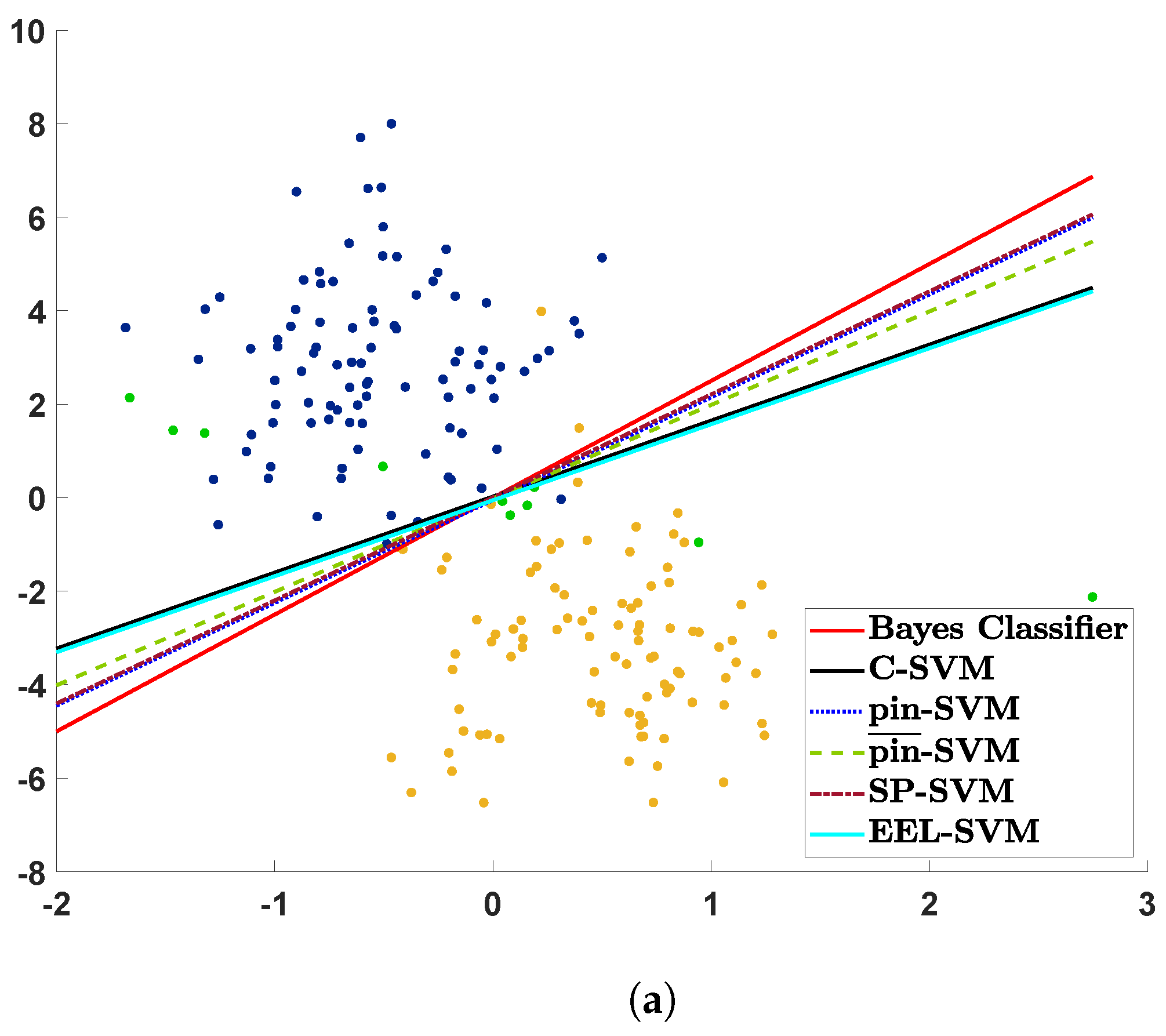
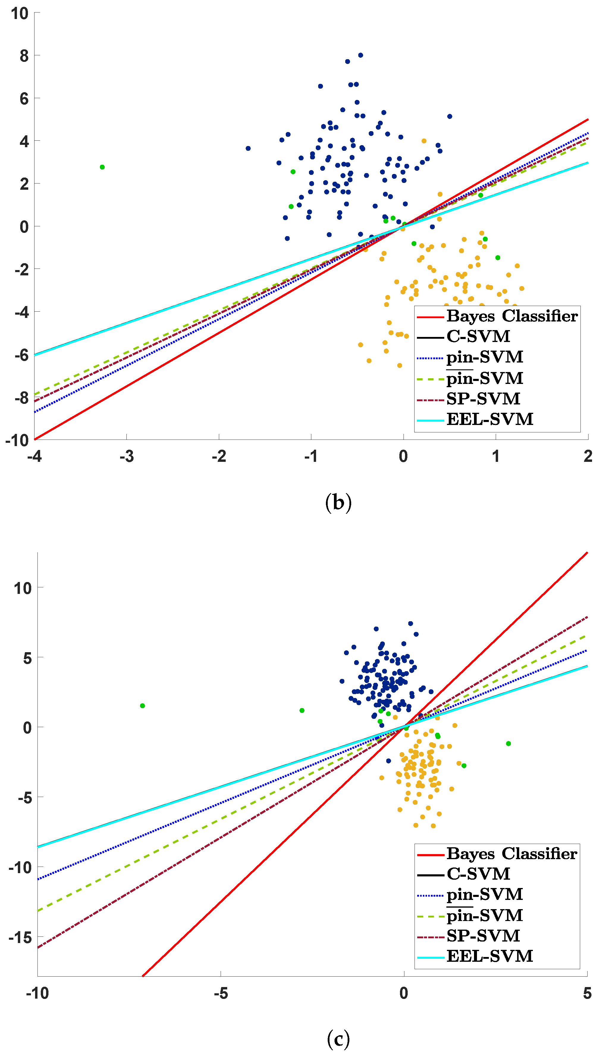
The contaminated data are plotted in Figure 1 together with their estimated decision lines. The three scatter plots visualize the realization of a sample of size $N=200$ that is contaminated with $r=5\%$, and the contaminated points appear in green. If a decision rule is close to the ‘true’ decision rule given by the red solid line, then we could say that its corresponding SVM classifier is more resilient to contamination, i.e., is more robust. Note that C-SVM and EEL-SVM overlap in Figure 1 because the contaminated data points become outliers that are too extreme, even for EEL-SVM, and, thus, this finds the same decision rule as C-SVM. Figure 1a shows that most of the classifiers, except C-SVM and EEL-SVM, are close to the ‘true’ classifier when a low level of DU is present due to the light-tailed Gaussian contamination; the same behavior is observed in Figure 1b, where a medium level of DU is present due to Student’s t with 5 degrees of freedom contamination. Recall that, the lower the number of degrees of freedom is, the more heavy-tailed Student’s t distribution is; therefore, Figure 1c illustrates the effect of a high level of DU, a case in which SP-SVM seems to be the most robust classifier.

The scatter plots in Figure 1 explain the contamination mechanism, though these pictorial representations may be misleading due to the sampling error, since Figure 1 relies on a single random sample. Therefore, we repeated the same exercise 100 times in order to properly compare the classifiers in

Table 2. Distance (13) between various SVM classifiers and Bayes classifier for contaminated synthetic data. Lowest distance along each row in bold.

	Normal distribution
	$r=0.05$			$r=0.10$
	$N=50$	$N=100$	$N=200$	$N=50$	$N=100$	$N=200$
C-SVM	1.3443	0.8397	0.6623	1.9649	1.1455	0.8675
$pin$-SVM	0.0537	0.0704	0.1880	0.5350	0.2955	0.2996
$\overline{pin}$-SVM	0.6378	0.3073	0.3984	1.2398	0.7334	0.4611
SP-SVM	0.3574	0.2305	0.2994	1.0827	0.5938	0.2813
EEL-SVM	1.3432	0.8431	0.6788	1.8921	1.1682	0.8785
	Student’s t distribution (5 degrees of freedom)
	$r=0.05$			$r=0.10$
	$N=50$	$N=100$	$N=200$	$N=50$	$N=100$	$N=200$
C-SVM	1.5685	1.1520	0.6795	2.4753	1.4983	0.9863
$pin$-SVM	0.8546	0.2966	0.1710	2.1801	0.6861	0.3322
$\overline{pin}$-SVM	1.2229	0.5929	0.3410	1.6040	0.9491	0.6492
SP-SVM	0.7485	0.7405	0.3754	1.3408	0.8801	0.4539
EEL-SVM	1.5901	1.1560	0.6895	2.4864	1.5077	1.0025
	Student’s t distribution (1 degree of freedom)
	$r=0.05$			$r=0.10$
	$N=50$	$N=100$	$N=200$	$N=50$	$N=100$	$N=200$
C-SVM	1.7930	1.8189	2.0358	3.1206	2.6941	3.2549
$pin$-SVM	0.8546	1.1983	1.6466	2.1801	2.0853	2.1472
$\overline{pin}$-SVM	1.2002	1.4458	1.3479	2.5982	1.9612	2.4647
SP-SVM	0.4277	1.2384	1.2675	2.1628	1.8261	1.8463
EEL-SVM	1.7669	1.8558	2.0280	3.0685	2.6788	3.2757

and

Table 3. Computational time ratios of SVM classifiers compared to C-SVM classifier for contaminated synthetic data. Lowest computational time ratio along each row in bold.

	Normal distribution
	$r=0.05$			$r=0.10$
	$N=50$	$N=100$	$N=200$	$N=50$	$N=100$	$N=200$
$pin$-SVM	4.2695	15.5138	33.9715	4.4855	19.2942	39.8558
$\overline{pin}$-SVM	2.5515	30.1658	22.9012	3.2739	36.6373	32.7994
SP-SVM	2.8101	7.6634	15.3068	2.9372	9.2248	16.7844
EEL-SVM	2.0301	6.6263	14.0950	2.1713	8.6631	16.1476
	Student’s t distribution (5 degrees of freedom)
	$r=0.05$			$r=0.10$
	$N=50$	$N=100$	$N=200$	$N=50$	$N=100$	$N=200$
$pin$-SVM	3.1421	12.6893	41.3835	4.4825	17.0174	44.2939
$\overline{pin}$-SVM	2.4289	42.1007	26.7222	4.0141	61.5340	27.6636
SP-SVM	2.2494	6.1618	19.6716	2.9885	7.7810	17.8432
EEL-SVM	2.3466	5.6473	17.2680	3.1776	7.7076	17.6688
	$r=0.05$			$r=0.10$
	$N=50$	$N=100$	$N=200$	$N=50$	$N=100$	$N=200$
$pin$-SVM	3.2366	11.4355	34.5926	4.4800	15.0441	41.0832
$\overline{pin}$-SVM	3.4272	25.4353	42.4561	5.6555	45.9922	62.0633
SP-SVM	2.4380	5.9118	15.5805	3.0326	7.3598	17.8881
EEL-SVM	2.1472	5.1893	14.5320	3.0242	7.1204	16.3805

. Moreover, for each sample, we conducted 10-fold cross-validation to tune the additional parameters, and we then computed the linear decision rule. The performance was measured via the distance (13), and the summary of this analysis is provided in Table 2 for samples of size $N\in \{50,100,200\}$ and a contamination ratio $r\in \{0.05,0.10\}$. Note that the tuning parameters were calibrated as in Section 4.1.1, except EEL-SVM, where the parameter space was enlarged (due to data contamination) as follows:

$${\mathcal{A}}_{EEL}:=\left\{\begin{array}{cc}\{0,0.01,\cdots ,0.05\}& \mathrm{if}r=0.05;\\ \{0,0.01,\cdots ,0.10\}& \mathrm{if}r=0.10.\end{array}\right.$$

EEL-SVM requires a larger parameter space when DU is more pronounced, i.e., $r=0.10$, but even in this extreme case, the cardinality of ${\mathcal{A}}_{EEL}$ is not larger than the cardinality of any other parameter space. That is, we did not favor EEL-SVM in the implementation phase.

Table 2 shows that the performance of any classifier deteriorates when the level of DU increases; moreover, the distance from the Bayes classifier increases with the contamination ratio r. The overall performances of SP-SVM and $pin$-SVM are superior to all three other competitors, whereas $\overline{pin}$-SVM appears to be competitive in just a few cases and C-SVM and EEL-SVM have a similar low performance. SP-SVM is by far the most robust classifier when DU is more pronounced, which is observed in Figure 1c but for a single sample.

We conclude our comparison by looking into the computational time ratios (with C-SVM as the baseline reference) that are reported in Table 3. In particular, this provides the computational times after tuning each model, i.e., the training computational time, which is a standard and fair reporting when one would expect high computational times when tuning more model hyper-parameters. The reference computational time (in sec) of the C-SVM, for a machine with Inter(R) Core(TM) i7−1065G7 CPU @ 1.30GHz, is approximately 0.0019 for $N=50$, 0.004 for $N=100$ and 0.0081 for $N=200$. EEL-SVM requires the lowest computational effort, though it is very close to SP-SVM, whereas $pin$-SVM is consistently slower and $\overline{pin}$-SVM is by far the method with the largest computational time. These observations are not surprising because $\overline{pin}$-SVM relies on a non-convex (DCA) algorithm that has scalability issues; on the contrary, $pin$-SVM, SP-SVM and EEL-SVM are solved via a convex LCQP of the same dimension, though EEL-SVM and $pin$-SVM are, respectively, the most and least sparse.

4.2. Real Data Analysis

We now compare the classification accuracy for some real-life data and rank all six SVM classifiers, including Ramp-KSVCR. Ten well-known real-world datasets are chosen in this section, which can be retrieved from the UCI depository1 and LIBSVM depository2; a summary is given in

Table 4. Summaries of UCI datasets.

	Data	Number of	Training	Testing
		Features	Sample Size	Sample Size
(I)	Fourclass	2	580	282
(II)	Diabetes	8	520	248
(III)	Breast cancer	10	460	223
(IV)	Australian	14	470	220
(V)	Statlog	13	180	90
(VI)	Customer	7	300	140
(VII)	Trial	17	520	252
(VIII)	Banknote	4	920	452
(IX)	A3a	123	3185	29,376
(X)	Mushroom	112	2000	6124

. It should be noted that all datasets had features rescaled to $[-1,1]$. Moreover, the analysis was carried out over the original and contaminated data. DU was introduced via the MATLAB R2019a function awgn with different signal noise ratios (SNR); perturbations were separately introduced 10 times for each dataset before training; and the average classification accuracy was reported so that the sampling error was alleviated.

The data were randomly partitioned into the training and testing sets, as described in Table 4. All SVM methods rely on the radial basis function (RBF) kernel chosen to overcome the lack of linearity in the data. As before, SP-SVM methodology assumes that the feature with the largest standard deviation is the one mostly affected by DU. All hyper-parameters were tuned via a 10-fold cross-validation; the kernel parameter $\gamma$ and penalty parameter C were tuned by allowing $\gamma ,C\in \left\{2^{-9},2^{-8},\cdots ,2^8,2^9\right\}$ for C-SVM, whereas $C\in \left\{2^{-5},2^{-3},2^{-1},2^0,2^1,2^3,2^5\right\}$ and $\gamma \in \left\{2^{-7},2^{-5},2^{-3},2^{-1},2^0,2^1\right\}$ are allowed for all other classifiers. Note that C-SVM has fewer parameters than other classifiers, and, thus, $(\gamma ,C)$ are allowed more values in the tuning process, so that all classifiers are treated as equally as possible. Note that Ramp-KSVCR has two penalty parameters $C_1,C_2$, an insensitivity parameter $ϵ$ and two additional model parameters s and t; the penalty parameters satisfy $C_1=C_2$, as in the original paper. The other parameters were tuned as follows:

• SP-SVM: $\alpha \in {\mathcal{A}}_{SP}=\{0.50,0.51,\cdots ,0.56,0.58,0.60\}$;
• EEL-SVM: $\alpha \in {\mathcal{A}}_{EEL}=\{0,0.05,0.10,\cdots ,0.3\}$;
• $pin$-SVM: $\tau \in {\mathcal{T}}_{pin}=\{0.1,0.2,\cdots ,0.8,1\}$;
• $\overline{pin}$-SVM$:s\in \{0.01,0.1,0.3,0.5,0.7,1\}$ and $\tau =0.5$;
• Ramp-KSVCR: $ϵ\in \{0.1,0.2,0.3\},t\in \{1,3,5\},s=-1$.

A final note is that a computational budget of around 370 parameter combinations was imposed on all cases, except EEL-SVM, where 294 combinations were considered.

Table 5. Classification accuracy (in %) of all SVM classifiers across all datasets. Highest accuracies along each row in bold. Each row signifies the original data (reported as “NA”, i.e., no contamination) or their contaminated variants (with SNR values 1, 5, 10).

Data	SNR	C-	pin-	$\overline{\mathit{pin}}$-	SP-	EEL-	Ramp-
		SVM	SVM	SVM	SVM	SVM	KSVCR
(I)	NA	99.29%	99.29%	99.65%	99.65%	99.65%	92.20%
	10	99.65%	99.65%	99.65%	99.61%	99.75%	91.95%
	5	99.65%	99.65%	99.65%	99.54%	99.72%	91.67%
	1	99.54%	99.61%	99.61%	99.50%	99.65%	91.84%
(II)	NA	77.02%	79.84%	79.84%	80.24%	78.63%	80.24%
	10	76.98%	76.49%	78.10%	79.64%	77.26%	77.10%
	5	76.69%	76.57%	77.54%	78.02%	76.45%	79.48%
	1	76.49%	77.70%	76.90%	77.66%	74.96%	79.44%
(III)	NA	93.72%	93.27%	94.17%	94.62%	93.72%	95.96%
	10	93.90%	94.75%	93.86%	93.32%	94.44%	95.29%
	5	93.86%	94.57%	94.17%	94.13%	94.08%	94.80%
	1	93.81%	93.86%	93.86%	93.86%	94.04%	95.11%
(IV)	NA	88.64%	88.18%	89.55%	88.18%	89.09%	89.55%
	10	85.82%	85.23%	85.77%	85.45%	85.32%	83.82%
	5	80.68%	80.50%	82.41%	80.59%	78.45%	77.73%
	1	76.59%	75.86%	77.86%	76.14%	76.23%	75.77%
(V)	NA	82.22%	82.22%	82.22%	83.33%	78.89%	80.00%
	10	80.22%	80.56%	77.56%	80.22%	82.44%	81.00%
	5	80.00%	79.33%	79.89%	79.33%	81.33%	77.00%
	1	78.67%	78.22%	80.00%	78.44%	76.89%	80.22%
(VI)	NA	92.14%	91.43%	90.71%	92.14%	92.86%	91.89%
	10	92.86%	92.50%	92.50%	92.71%	93.21%	89.93%
	5	92.93%	92.86%	91.43%	93.07%	93.07%	91.36%
	1	92.57%	92.93%	91.57%	92.57%	92.86%	90.79%
(VII)	NA	100.00%	100.00%	100.00%	100.00%	100.00%	100.00%
	10	99.56%	99.80%	99.33%	99.76%	99.60%	99.48%
	5	94.72%	94.60%	94.44%	94.84%	94.52%	93.97%
	1	88.13%	88.13%	85.99%	88.29%	88.21%	86.98%
(VIII)	NA	100.00%	100.00%	100.00%	100.00%	100.00%	100.00%
	10	99.73%	99.71%	99.80%	99.76%	99.89%	99.85%
	5	99.38%	99.18%	99.05%	99.25%	99.36%	99.05%
	1	97.94%	97.92%	97.61%	97.94%	97.83%	96.75%
(IX)	NA	82.81%	83.20%	83.36%	83.67%	81.71%	84.04%
	10	80.50%	81.05%	80.57%	81.12%	81.15%	81.13%
	5	78.57%	78.56%	77.94%	78.35%	78.26%	78.00%
	1	76.34%	76.74%	75.94%	76.01%	76.02%	76.25%
(X)	NA	99.87%	99.87%	99.87%	99.87%	99.87%	99.87%
	10	98.37%	98.84%	99.38%	98.31%	98.29%	99.03%
	5	93.02%	93.79%	94.72%	93.05%	92.92%	93.77%
	1	85.36%	85.63%	85.82%	85.46%	85.47%	85.55%
Average rank		3.25	3.18	3.18	2.93	3.05	3.53

summarizes the classification performance for all ten datasets for the original (non-contaminated) data and their contaminated variants with various SNR values, where a smaller SNR value means a higher degree of data contamination. EEL-SVM achieves the best performance in 14 out of 40 scenarios investigated, which is followed by Ramp-KSVCR, which performs best in 13 out of 40 scenarios; the other classifiers are ranked as follows: SP-SVM (11/40), $\overline{pin}$-SVM (10/40), C-SVM (7/40) and $pin$-SVM (6/40). We also calculated the average ranks for each classifier by looking at each row of Table 5 and ranking each entry from 1 to 6 from lowest to highest accuracy; SP-SVM and EEL-SVM yield the best average ranks among all classifiers and SP-SVM outperforms its competitors via this criterion.

We also performed a statistical test to verify whether the performances produced by one method are significantly better than the others on these datasets. In particular, the right-tailed paired sample t-test was considered. Under the null hypothesis, the difference between the paired population means is equal to 0. Conversely, the alternative hypothesis states that this difference is greater than 0. The tests were conducted considering all of the results reported in Table 5, and the corresponding p-values are shown in

Table 6. p-Values of right-tailed paired sample t-tests. Values lower than $0.05$ are bold.

	C-	pin-	$\overline{\mathit{pin}}$-	SP-	EEL-	Ramp-
	SVM	SVM	SVM	SVM	SVM	KSVCR
C-SVM		0.8349	0.7345	0.9688	0.3605	0.0506
$pin$-SVM	0.1651		0.5105	0.8881	0.1815	0.0268
$\overline{pin}$-SVM	0.2655	0.4895		0.8008	0.2668	0.0320
SP-SVM	0.0312	0.1119	0.1992		0.0714	0.0123
EEL-SVM	0.6395	0.8185	0.7332	0.9286		0.0721
Ramp-KSVCR	0.9494	0.9732	0.9680	0.9877	0.9279

. Each table cell reports the p-value obtained by testing the performances of the row against the column models as indicated. We set the significance level equal to 5% and reported p-values below this in bold. Interestingly, we observed that $pin$-SVM, $\overline{pin}$-SVM and SP-SVM perform significantly better than Ramp-KSVCR. Furthermore, we observed that the p-values associated with SP-SVM are generally lower than the other methods. Indeed, SP-SVM is the only method that also outperforms C-SVM, making it preferable to other strong competitors.

In summary, despite the EEL-SVM performing very well on the real-world data, we conclude that SP-SVM exhibits a competitive advantage over competitors.

4.3. Interpretable Classifiers

The performance of SVM classifiers for real-life data has been analyzed in Section 4.2 without interpreting the decision rules so that the presence of DU is better understood and the fairness of the decision is assessed. We achieved that now by providing a granular analysis for the classification of the following two sources of data:

• US mortgage lending data that are downloaded from the Home Mortgage Disclosure Act (HMDA) website3; specifically, we collected the 2020 data for two states, namely, Maine (ME) and Vermont (VT), with a focus on subordinated lien mortgages;
• Insurance fraud data named car insurance (CI) that are available on Kaggle website4.

The US mortgage lending data refer to subordinate-lien (‘piggyback’) loans that are taken out at the same time as first-lien mortgages on the same property by borrowers, mainly to avoid paying mortgage insurance on the first-lien mortgage (due to the extra down payment). Eriksen et al. (2013) find evidence that borrowers with subordinate loans have an increased-by-62.7% chance to default each month on their primary loan. Such borrowers may sequentially default on each loan since subordinate lenders will not pursue foreclosure if the borrowers have insufficient equity until at least housing markets start to recover. Subordinate-lien loans are high-risk mortgages and we aimed to classify the instances as ‘loan originated’ ($Y=+1$) or ‘application denied’ ($Y=-1$) using the available features. The HMDA data have numerous features and the following representative ones were chosen: (F1) loan amount, (F2) loan-to-value ratio (F1 divided by the ‘property_value’), (F3) percentage of minority population to total population for tract, (F4) percentage of tract median family income compared to MSA (metropolitan statistical area) median family income. Two categorical features were also considered, namely, (F5) derived sex and (F6) age.

The insurance fraud detection data refer to motor insurance claims, and the aim was to identify if a claim is fraudulent ($Y=-1$) or not ($Y=+1$). The CI dataset is quite balanced since $25\%$ of the claims are recorded as fraudulent. Several features were available, and a preliminary round of features engineering was performed. We considered the following numerical features: (G1) the age of the policyholder, (G2) the percentage of the ‘injury_claim’ on the total claim amount, (G3) the percentage of the ‘vehicle_claim’ on the total claim amount, (G4) the total claim amount and (G5) the age of the vehicle at the time of the incident. The last one was computed as the period between the ‘auto_year’ (the year of registration of the vehicle) and the ‘incident_date’. In addition, we included the categorical features related to the policy, namely, (G6) the state and (G7) the deductible; related to the insured, namely, (G8) the gender, (G9) educational level and (G10) relationship; and, related to the incident, that is, (G11) type, G12) severity and (G13) state.

All categorical features (of the two sources of data) were pre-processed via standard one-hot encoding procedure and all features were rescaled to $[-1,1]$ before training. Random sampling was performed to extract the training and testing sets, so that the training set was twice as large as the testing set. The hyper-parameter tuning of the three methods (C-SVM, SP-SVM, EEL-SVM) was performed via 10-fold cross-validation using the hyper-parameter spaces in Section 4.2. SP-SVM identifies F1 (loan amount) and G4 (claim amount) as the features affected by DU that have the largest standard deviation at the same time. This is not surprising since both features have a massive impact on the target variable and they are heavily influenced by all other features.

Table 7. Summaries of HMDA datasets and their accuracy levels. Highest accuracy along each row in bold.

Dataset	Total	Testing	C-SVM	SP-SVM	EEL-SVM
	Sample Size	Sample Size
ME	4226	1396	70.77%	70.77%	70.13%
VT	1948	648	90.74%	91.67%	90.89%
CI	1000	330	83.33%	83.33%	83.93%

reports the details of the training–testing splitting and the out-of-sample accuracy of the three SVM methods.

We observed that EEL-SVM obtains the best result for the CI data, whereas SP-SVM performs best in terms of accuracy, with C-SVM and EEL-SVM relatively close. The next step was to interpret the classification rule and explain the DU effect, but also to evaluate the effect of an automatized mortgage lending decision. The latter was measured by looking into unfavorable decisions where the loan is denied, i.e., $Y=-1$.

The Equal Credit Opportunity Act (ECOA) prohibits a creditor from discriminating against any borrower on the basis of age, marital status, race, religion or sex, known as protected characteristics; such a regulatory requirement is imposed not only in the US, but also similar ones are in place in the EU, UK and elsewhere. Under ECOA, regulatory agencies assess the lending decision fairness of lending institutions by comparing the unfavorable decision ($Y=-1$) across different groups with given protected characteristics. Our next analysis focuses on checking whether an automatized lending decision could lead to unintentional discrimination, known as disparate impact. First, we looked at the entry data and provided evidence on whether or not the loan amount is massively different across the applicants’ gender at birth, income and racial structure in their postal code, which would explain if DU is present or not. Second, we evaluated the fairness of the lending decision obtained via SVM classification and argued which SVM-based decision is more compliant with such non-discrimination regulation (with respect to the sex attribute).

Table 8. Kolmogorov–Smirnov distances in loan amount distributions of males versus females (MvsF), males versus joint (MvsJ) and females versus joint (FvsJ). Largest distances along each row corresponding to training and testing data in bold.

		Training Data			Testing Data
		MvsF	MvsJ	FvsJ	MvsF	MvsJ	FvsJ
ME	$Y\in \{-1,1\}$	0.0853	0.0477	0.1330	0.0969	0.1248	0.2096
	$Y=-1$	0.0540	0.0727	0.1215	0.1203	0.1122	0.2313
	$Y=1$	0.1091	0.0381	0.1472	0.0889	0.1266	0.1986
VT	$Y\in \{-1,1\}$	0.0923	0.1009	0.1841	0.1355	0.1399	0.2000
	$Y=-1$	0.0866	0.0449	0.1208	0.3095	0.1429	0.1667
	$Y=1$	0.1258	0.1579	0.2515	0.1235	0.1575	0.2108

reports the Kolmogorov–Smirnov distances for loan amount samples of applicants based on gender characteristics. There is overwhelming evidence that joint loan applications and female applicants have very different loan amount distributions in both training and testing data, though VT data exhibit the largest distance when comparing male and female applicants with a favorable mortgage lending decision. This could be explained by socio-economic disparities between males and females, though DU plays a major role in this instance. Gender information in the HMDA data is expected to have a self-selection bias, since applicants at risk are quite unlikely to report gender information as they believe that the lending decision would be influenced by that. Consequently, we removed a significant portion of the data, i.e., examples for which the gender information is unknown, which is clear evidence of self-selection bias in our entry data.

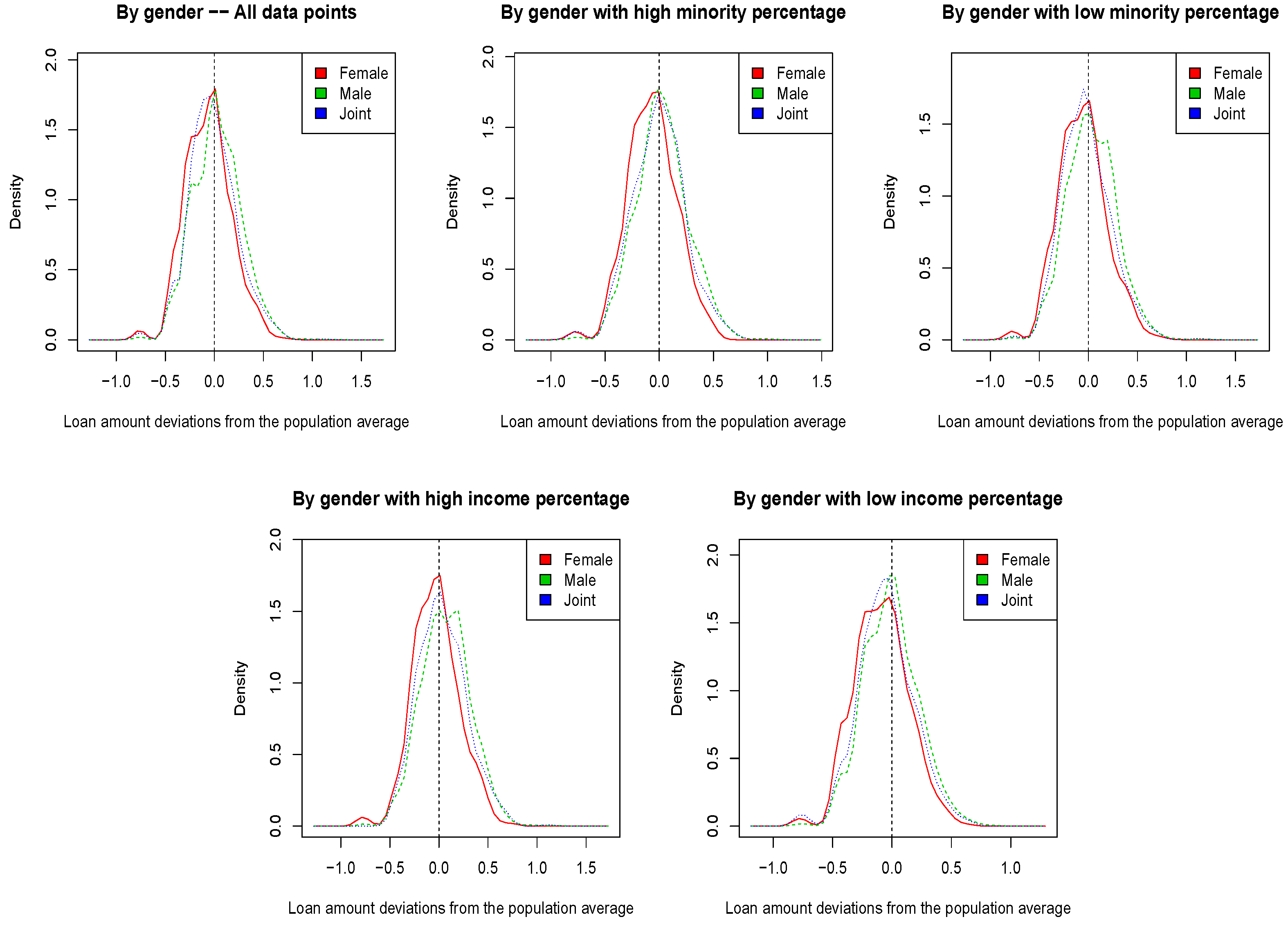
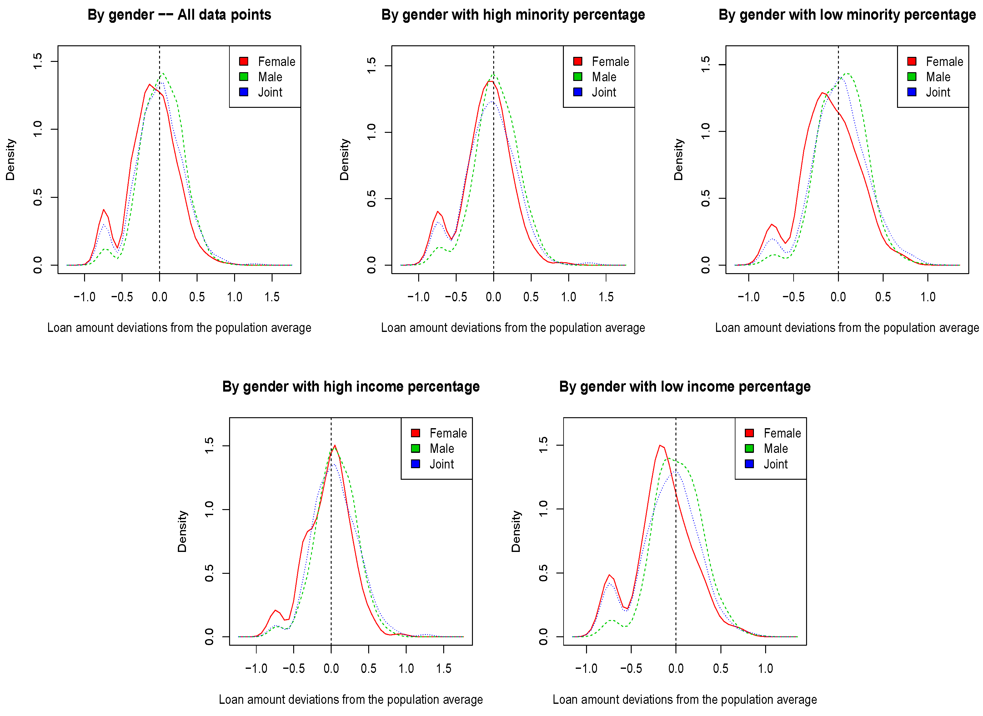
Figure 2 and Figure 3 show the kernel densities of the deviation in the log-transformed loan amount from the population mean. In particular, we plotted such deviations for the entire dataset, but also for sub-populations with a low/high minority and income percentage. A low/high minority percentage means that the mortgage applicant is in an area of lower/higher minority than the population median. Moreover, a low/high income percentage means that the mortgage applicant household income is lower/higher than the household income in her/his MSA. ME data from Figure 2 do not show any evidence of DU with respect to the loan amount, which explains the results in Table 7, where SP-SVM and EEL-SVM did not improve the non-robust counterpart. VT data show a very different scenario in Figure 3, where the loan amount deviations have a bimodal distribution. In addition, within the low minority sub-population, female applicants exhibit significantly lower loan amounts than all other applicants; the same pattern is observed in the low income sub-population. Therefore, the DU in the VT data is evident, and confirms the findings in Table 8, but also those in Table 7, where SP-SVM and EEL-SVM did improve the non-robust C-SVM.

We have concluded the first part of our qualitative analysis, where we have explained the DU, and we now evaluate how compliant the automatized mortgage lending process would be for the VT data; we do not report the ME results due to a lack of DU. Fairness compliance requires the lending decision—especially the unfavorable decisions ($Y=-1$)—to be independent of the applicant’s gender at birth information, i.e.,

$$Pr(Y=-1)=Pr(Y=-1|S=l)\mathrm{for}\mathrm{all}l\in \mathcal{S}:=\{Female,Male,Joint\}.$$

(14)

Table 9. Probability of denied loan for the three classification methods. Closest value (per row) to ‘true’ probability in bold.

	C-SVM	SP-SVM	EEL-SVM	True
$Pr(Y=-1)$	2.3148%	1.0802%	5.5556%	7.8704%
$Pr(Y=-1|\mathrm{Female})$	3.9683%	1.5873%	6.3492%	9.5238%
$Pr(Y=-1|\mathrm{Male})$	7.8125%	3.9063%	10.1563%	16.4062%
$Pr(Y=-1|\mathrm{Joint})$	0.0000%	0.0000%	3.8071%	4.5685%
$Pr(Y=-1|\mathrm{Low}\mathrm{Income})$	2.9316%	0.9772%	5.5375%	8.0495%
$Pr(Y=-1|\mathrm{High}\mathrm{Income})$	1.7595%	1.1730%	5.5718%	7.6923%
$Pr(Y=-1|\mathrm{Low}\mathrm{Minority})$	1.8576%	0.9290%	5.5728%	9.7720%
$Pr(Y=-1|\mathrm{High}\mathrm{Minority})$	2.7692%	1.2308%	5.5385%	6.1584%
$CDD$	−25.5944%	−25.2601%	−8.3263%	−11.3792%

tells us that the desirable lack of disparity in (14) is achieved best by EEL-SVM. In addition, EEL-SVM estimates the unfavorable decisions very similarly to the ‘true’ decisions, and this can be seen by inspecting the probabilities that appear in bold.

One popular fairness metric is the conditional demographic disparity (CDD), which is discussed in Wachter et al. (2021), where the data are assumed to be part of multiple strata. The CDD formulation for our data (with three strata, i.e., female, male and joint) is defined as

$$\mathrm{CDD}=\sum _{l\in \mathcal{S}}Pr(S=l)\times D{D}_l,$$

where $D{D}_l$ is the demographic disparity within the $l^{th}$ stratum, i.e.,

$$D{D}_l=Pr(S=l\mid Y=-1)-Pr(S=l\mid Y=1)\mathrm{for}\mathrm{all}l\in \mathcal{S}.$$

CDD could capture and explain peculiar data behavior similar to Simpson’s paradox, where the same trend is observed in each stratum, but the opposite trend is observed in the whole dataset. Amazon SageMaker, a cloud machine-learning platform developed by Amazon, has included CDD in their practice to enhance model explainability and bias detection; for details, see the Amazon SageMaker Developer Guide.

Table 9 shows that EEL-SVM has a superior performance to C-SVM and SP-SVM when looking at the overall CDD fairness performance. In fact, EEL-SVM exhibits fairer post-training decisions than the pre-training fairness measured on the ‘true’ mortgage lending decisions observed in the testing data. In summary, the unanimous conclusion is that EEL-SVM shows the fairest and most robust mortgage-lending automatized decision.

5. Concluding Remarks

This paper examines the binary classification problem in the context of data uncertainty. Two powerful SVM-type classification algorithms are developed and discussed: the SP-SVM and EEL-SVM. A large set of numerical experiments have been conducted to test their effectiveness on synthetic and real-world datasets, both with and without noise contamination.

Their performances have been compared with the classical C-SVM and some well-known robust SVM formulations from the literature: $pin$-SVM, $\overline{pin}$-SVM and the Ramp-KSVCR. The results highlight that both our newly proposed methods are promising alternatives to those currently available in the literature. SP-SVM achieved good results in all our experiments, especially on synthetic data with strong noise contamination. EEL-SVM was found to be less competent in synthetic experiments, but appeared to be an accurate classifier for real-world datasets. In addition, the training of these two methods includes optimization problems that can be efficiently solved faster than for other SVM methods. We also showed empirically, using economic and insurance data, that both proposed methods can lead to an interesting gain in classification accuracy when the data are affected by DU.

Future research will proceed in different directions. First, we plan to extend the proposed methods to multiclass classification problems. Second, we intend to develop a new SVM extension that combines the benefits of SP-SVM and EEL-SVM; this can be a useful tool for handling very noisy data. Finally, we aim to explore new SVM formulations that are robust to non-symmetric distributed noise.

References

1. Artis, Manuel, Mercedes Ayuso, and Montserrat Guillen. 1999. Modelling different types of automobile insurance fraud behaviour in the Spanish market. Insurance: Mathematics and Economics 24: 67–81. [Google Scholar] [CrossRef]
2. Asimit, Alexandru V., Valeria Bignozzi, Ka Chun Cheung, Junlei Hu, and Eun-Seok Kim. 2017. Robust and Pareto optimality of insurance contracts. European Journal of Operational Research 262: 720–32. [Google Scholar] [CrossRef]
3. Bamakan, Seyed Mojtaba Hosseini, Huadong Wang, and Yong Shi. 2017. Ramp loss K-support Vector Classification-Regression; a robust and sparse multi-class approach to the intrusion detection problem. Knowledge-Based Systems 126: 113–26. [Google Scholar] [CrossRef]
4. Bartlett, Peter L., Michael I. Jordan, and Jon D. McAuliffe. 2006. Convexity, classification, and risk bounds. Journal of the American Statistical Association 101: 138–56. [Google Scholar] [CrossRef] [Green Version]
5. Bermudez, Lluis, Jeanneth Perez, Mercedes Ayuso, Esther Vázquez Gomez, and Francisco José Vazquez. 2008. A Bayesian dichotomous model with asymmetric link for fraud in insurance. Insurance: Mathematics and Economics 42: 779–86. [Google Scholar] [CrossRef]
6. Bertsimas, Dimitris, Jack Dunn, Colin Pawlowski, and Ying Daisy Zhuo. 2018. Robust classification. Journal on Optimization 1: 2–34. [Google Scholar] [CrossRef] [Green Version]
7. Bi, Jinbo, and Tong Zhang. 2005. Support vector classification with input data uncertainty. In Advances in Neural Information Processing Systems. Cambridge: MIT Press, pp. 161–68. [Google Scholar]
8. Cortes, Corinna, and Vladimir Naumovich Vapnik. 1995. Support-vector networks. Machine Learning 20: 273–97. [Google Scholar] [CrossRef]
9. Eriksen, Michael D., James B. Kau, and Donald C. Keenan. 2013. The impact of second loans on subprime mortgage defaults. Real Estate Economics 41: 858–86. [Google Scholar] [CrossRef]
10. Fan, Jianqing, Yuan Liao, and Han Liu. 2016. An overview of the estimation of large covariance and precision matrices. The Econometrics Journal 19: C1–C32. [Google Scholar] [CrossRef]
11. Fang, Kai-Tai, Samuel Kotz, and Kai Wang Ng. 1990. Symmetric Multivariate and Related Distributions. Boca Raton: Chapman & Hall/CRC. [Google Scholar]
12. Huang, Gao, Shiji Song, Cheng Wu, and Keyou You. 2012. Robust support vector regression for uncertain input and output data. IEEE Transactions on Neural Networks and Learning Systems 23: 1690–700. [Google Scholar] [CrossRef]
13. Huang, Xiaolin, Lei Shi, and Johan A. K. Suykens. 2014. Support vector machine classifier with pinball loss. IEEE Transactions on Pattern Analysis and Machine Intelligence 36: 984–97. [Google Scholar] [CrossRef] [PubMed]
14. Kallus, Nathan, Xiaojie Mao, and Angela Zhou. 2022. Assessing algorithmic fairness with unobserved protected class using data combination. Management Science 68: 1959–81. [Google Scholar] [CrossRef]
15. Lanckriet, Gert R. G., Laurent El Ghaoui, Chiranjib Bhattacharyya, and Michael I. Jordan. 2002. A robust minimax approach to classification. Journal of Machine Learning Research 3: 555–82. [Google Scholar]
16. Ledoit, Olivier, and Michael Wolf. 2020. The power of (non-) linear shrinking: A review and guide to covariance matrix estimation. Journal of Financial Econometrics 20: 187–218. [Google Scholar] [CrossRef]
17. Lin, Yi. 2002. Support vector machines and the Bayes rule in classification. Data Mining and Knowledge Discovery 6: 259–75. [Google Scholar] [CrossRef]
18. Lin, Yi. 2004. A note on margin-based loss functions in classification. Statistics & Probability Letters 68: 73–82. [Google Scholar]
19. Rockafellar, R. Tyrrell, and Stanislav Uryasev. 2000. Optimization of conditional value-at-risk. Journal of Risk 2: 21–42. [Google Scholar] [CrossRef] [Green Version]
20. Shen, Xin, Lingfeng Niu, Zhiquan Qi, and Yingjie Tian. 2017. Support vector machine classifier with truncated pinball loss. Pattern Recognition 68: 199–210. [Google Scholar] [CrossRef]
21. Singh, Abhishek, Rosha Pokharel, and Jose Principe. 2014. The C-loss function for pattern classification. Pattern Recognition 47: 441–53. [Google Scholar] [CrossRef]
22. Steenackers, Astrid, and Marc Goovaerts. 1989. A credit scoring model for personal loans. Insurance: Mathematics and Economics 8: 31–34. [Google Scholar] [CrossRef]
23. Suykens, Johan A. K., and Joos Vandewalle. 1999. Least squares support vector machine classifiers. Neural Processing Letters 9: 293–300. [Google Scholar] [CrossRef]
24. Vapnik, Vladimir Naumovich. 2000. The Nature of Statistical Learning Theory, 2nd ed. New York: Springer. [Google Scholar]
25. Wachter, Sandra, Brent Mittelstadt, and Chris Russell. 2021. Why fairness cannot be automated: Bridging the gap between eu non-discrimination law and ai. Computer Law & Security Review 41: 105567. [Google Scholar] [CrossRef]
26. Wang, Ximing, Neng Fan, and Panos M. Pardalos. 2018. Robust chance-constrained support vector machines with second-order moment information. Annals of Operations Research 263: 45–68. [Google Scholar] [CrossRef]
27. Wu, Yichao, and Yufeng Liu. 2007. Robust truncated hinge loss support vector machines. Journal of the American Statistical Association 102: 974–83. [Google Scholar] [CrossRef] [Green Version]
28. Xu, Guibiao, Zheng Cao, Bao-Gang Hu, and Jose C. Principe. 2017. Robust support vector machines based on the rescaled hinge loss function. Pattern Recognition 63: 139–48. [Google Scholar] [CrossRef]
29. Zhang, Tong. 2004. Statistical analysis of some multi-category large margin classification methods. Journal of Machine Learning Research 5: 1225–51. [Google Scholar]
30. Zhang, Yan. 2016. Assessing fair lending risks using race/ethnicity proxies. Management Science 64: 178–97. [Google Scholar] [CrossRef]
Figure 1. Classification boundaries for five SVM classifiers if DU is induced by (a) normal distribution, (b) Student’s t distribution with 5 degrees of freedom and (c) Student’s t distribution with 1 degree of freedom.
Risks 10 00154 g001aRisks 10 00154 g001b
Figure 2. ME loan amount deviations from the population mean based on full data and sub-populations with low/high minority and low/high income percentages.
Risks 10 00154 g002
Figure 3. VT loan amount deviations from the population mean based on full data and sub-populations with low/high minority and low/high income percentages.
Risks 10 00154 g003