Article

Scenario Generation for Market Risk Models Using Generative Neural Networks

1
Deutsche Rueckversicherung AG, Market Risk Management, Hansaallee 177, 40549 Duesseldorf, Germany
2
Institut für Mathematik, Carl von Ossietzky Universität, 26111 Oldenburg, Germany
*
Author to whom correspondence should be addressed.
Risks 2022, 10(11), 199; https://doi.org/10.3390/risks10110199
Submission received: 11 July 2022 / Revised: 27 September 2022 / Accepted: 10 October 2022 / Published: 22 October 2022
(This article belongs to the Special Issue Data Science in Insurance)

Abstract

:
In this research study, we show how existing approaches of using generative adversarial networks (GANs) as economic scenario generators (ESG) can be extended to an entire internal market risk model—with enough risk factors to model the full band-width of investments for an insurance company and for a time horizon of one year, as required in Solvency 2. We demonstrate that the results of a GAN-based internal model are similar to regulatory-approved internal models in Europe. Therefore, GAN-based models can be seen as an alternative data-driven method for market risk modeling.

1. Introduction

Generating realistic scenarios of how financial markets might behave in the future is one key component of internal market risk models used by insurance companies for Solvency 2 purposes. Currently, these are built using economic scenario generators (ESGs) based mainly on financial mathematical models; see Bennemann (2011) and Pfeifer and Ragulina (2018). These ESGs require strong assumptions on the behavior of the risk factors and their dependencies, are time consuming to calibrate, and it is difficult in this framework to model complex dependencies.
An alternative method for scenario generation can be a special type of neural networks called generative adversarial networks (GANs) invented by Goodfellow et al. (2014). This network architecture consists of two neural networks, which has gained much attention due to its ability to generate realistic-looking images; see Aggarwal et al. (2021).
As financial data, at least for liquid instruments, are consistently available, GANs are used in various areas of finance, including market prediction, tuning trading models, portfolio management and optimization, synthetic data generation, and diverse types of fraud detection; see Eckerli and Osterrieder (2021). Henry-Labordere (2019), Lezmi et al. (2020), Fu et al. (2019), Wiese et al. (2019), Ni et al. (2020), and Wiese et al. (2020) have already used GANs for scenario generation in the financial sector. The focus of their research was the generation of financial time series for a limited number of risk factors (up to 6) or a single asset class. To the best of our knowledge, there is no research performing a full value-at-risk calculation for an insurance portfolio based on GAN-generated scenarios.
In this study, we perform a market risk calculation for typical insurance portfolios using a GAN instead of a classical ESG. We base our research on publicly available financial data from Bloomberg. The research of Ngwenduna and Mbuvha (2021), Cote et al. (2020) and Kuo (2019) also uses GAN in an actuarial context, but they use it to generate publicly available data from restricted data or to create new data for solving the issue of having imbalanced datasets. However, the methods introduced in those papers could be used when dealing with illiquid instruments where no consistent tabular data are available.
In this research study, we perform the following:
  • Expand scenario generation by a GAN to a complete market risk calculation for Solvency 2 purposes in insurance companies;
  • Compare the results of a GAN-based ESG to ESG approaches implemented in regulatory-approved market risk models in Europe.
As a novelty, this research study shows that there is an alternative method for market risk modeling beyond traditional ESGs, which can also serve as regulatory-approved models as they perform well in the EIOPA (European Insurance and Occupational Pensions Authority) benchmarking study. Therefore, the proof of concept of whether a GAN can serve as an ESG for market risk modeling is successful.
The paper is structured as follows: In Section 2, we provide some background both on market risk calculation under Solvency 2 and on GANs. The MCRCS (market and credit risk comparison study), a benchmarking exercise for approved market risk models in Europe conducted annually by EIOPA, is also introduced in Section 2. Section 3 explains how GANs can be used as ESGs and how they can be included in an internal model process. A comparison of the results of a GAN-based internal model with the results of the models in the MCRCS study and a discussion of the stability of these results is presented in this Section, as well. Section 4 explains the methodology and data used for the GAN-based model and how a GAN-based ESG can be implemented. Section 5 concludes and provides on overview of the differences of this GAN-based approach with traditional methods.

2. Background

Before we present our work, we provide a short introduction to the two main topics involved: economic scenario generators (ESG) and their usage for market risk calculation under Solvency 2 and generative adversarial networks (GANs).

2.1. Market Risk Calculation under Solvency 2

In 2016, a new regulation for insurance companies in Europe was introduced: Solvency 2. One central requirement is the calculation of the solvency capital requirement, called SCR. The amount of SCR depends on the risks to which the insurance company is exposed; see, e.g., Gründl et al. (2019, Chapter 4). The eligible capital of an insurance company is then compared with the SCR to determine whether the eligible capital is sufficient to cover all risks taken by the insurance company.
The solvency capital requirement equals the Value-at-Risk (VaR) at a 99.5%-level for a time horizon of one year; see Bennemann (2011, Chapter 2.3). A mathematical definition of the VaR and a derivation of its usage in this context can be found in Denuit et al. (2006, p. 69).
The risk of an insurer can be divided into six different modules: market risk, health underwriting risk, counterparty default risk, life underwriting risk, non-life underwriting risk and operational risk. The modules themselves consist of sub-modules; see EIOPA (2014). Market risk, e.g., consists of the six submodules: interest rate, equity, property, spread, currency and concentration risk.
The SCR can be calculated using either the standard model or an internal model. For the standard model, the regulatory framework sets specific rules for the calculation for each risk encountered by the insurance company, defined in European Commission (2015). Each internal model has to cover the same types of risks as the standard model and must be approved by local supervisors to ensure consistency with the principles of Solvency 2.
In this study, we will focus on the calculation of the market risk of a non-life insurer. However, the methods presented here can be applied for other risks as well. The reason for selecting market risk here is three-fold:
  • The underlying data in the financial market are publicly available and equal for all insurers;
  • Market risk forms a major part of the SCR of an insurance company (EIOPA (2021b, p. 22), which states that market risk accounts for 53% of the net solvency capital requirement before diversification benefits; this varies between life (59%) and non-life (43%) insurers);
  • A comprehensive benchmark exercise, called “market and credit risk comparison study” MCRCS conducted by EIOPA, is available for a comparison of the results.
Current internal models for market risk often use Monte-Carlo simulation techniques to derive the risk of the sub-modules and then use correlations or copulas for aggregation; see Bennemann (2011, p. 189) and Pfeifer and Ragulina (2018). The basis of the Monte-Carlo simulation is a scenario generation performed by an “economic scenario generator” ESG.
A definition of an ESG can be found in Pedersen et al. (2016, p. 7):
Definition 1.
An economic scenario generator (ESG) is a computer-based model of an economic environment that is used to produce simulations of the joint behavior of financial market values and economic variables.
The ESG implements financial-mathematical models for all relevant risk factors (e.g., interest rate and equity) and their dependencies. Under those scenarios, the investment and liability portfolio of the insurer is evaluated, and the risk is given by the 0.5% percentile of the loss in these scenarios.

2.2. Introduction to the MCRCS Study

Since 2017, EIOPA performs an annual study, called the market and credit risk comparison study (abbr. MCRCS). According to the instructions from EIOPA MCRCS Project Group (2020b), the “primary objective of the MCRCS is to compare market and credit risk model outputs for a set of realistic asset portfolios”. In the study, all insurance undertakings with significant exposure in EUR and with an approved internal model are asked to participate; see EIOPA (2021a). In the study as of year-end 2019, 21 insurance companies from eight different countries of the European Union participated.
All participants have to model the risk of 104 different synthetic instruments. Those comprise all relevant asset classes, i.e., risk-free interest rates, sovereign bonds, corporate bonds, equity indices, property, foreign exchange and some derivatives. A detailed overview of the synthetic instruments that are used in this study can be found in EIOPA MCRCS Project Group (2020a).
Additionally, those instruments are grouped into ten different asset-only benchmark portfolios, two liability-only benchmark portfolios and ten combined portfolios. These portfolios “should reflect typical asset risk profiles of European insurance undertakings”; see EIOPA MCRCS Project Group (2020b, Section 2). This analysis sheds light into the interaction and dependencies between risk factors.
These 22 portfolios are denoted as follows:
  • Asset-only benchmark portfolios: BMP1, BMP2, …, BMP10;
  • Liability-only benchmark portfolios: L1 and L2;
  • Combined portfolios: BMP1+L1, BMP3+L1, BMP7+L1, BMP9+L1, BMP10+L1, BMP1+L2, BMP3+L2, BMP7+L2, BMP9+L2 and BMP10+L2.
The combined portfolios are linear combinations of the asset and liability benchmark portfolios; e.g., BMP1+L1 combines the asset-only benchmark portfolio BMP1 with liability portfolio L1.
Figure 1 presents the asset-type composition of the asset-only benchmark portfolios.
All asset portfolios mainly consist of fixed income securities (86% to 94%) as this forms the main investment focus of insurance companies. However, there are significant differences both in ratings, durations and also in the weighting between sovereign and corporate exposures.
The two liability profiles are assumed to be zero-bond based, so they represent the liabilities of non-life insurance companies and differ in their durations (13.1 years vs. 4.6 years).
Annually, EIOPA publishes a detailed article of the MCRCS exercise. It provides an anonymized comparison of the risk charges of different insurance companies’ market risk models by portfolios, instruments and some additional analysis, e.g., dependencies of the risk factors. The study for year-end 2019 can be found on the EIOPA homepage; see EIOPA (2021a). We will use the results of this study for comparison in Section 3.

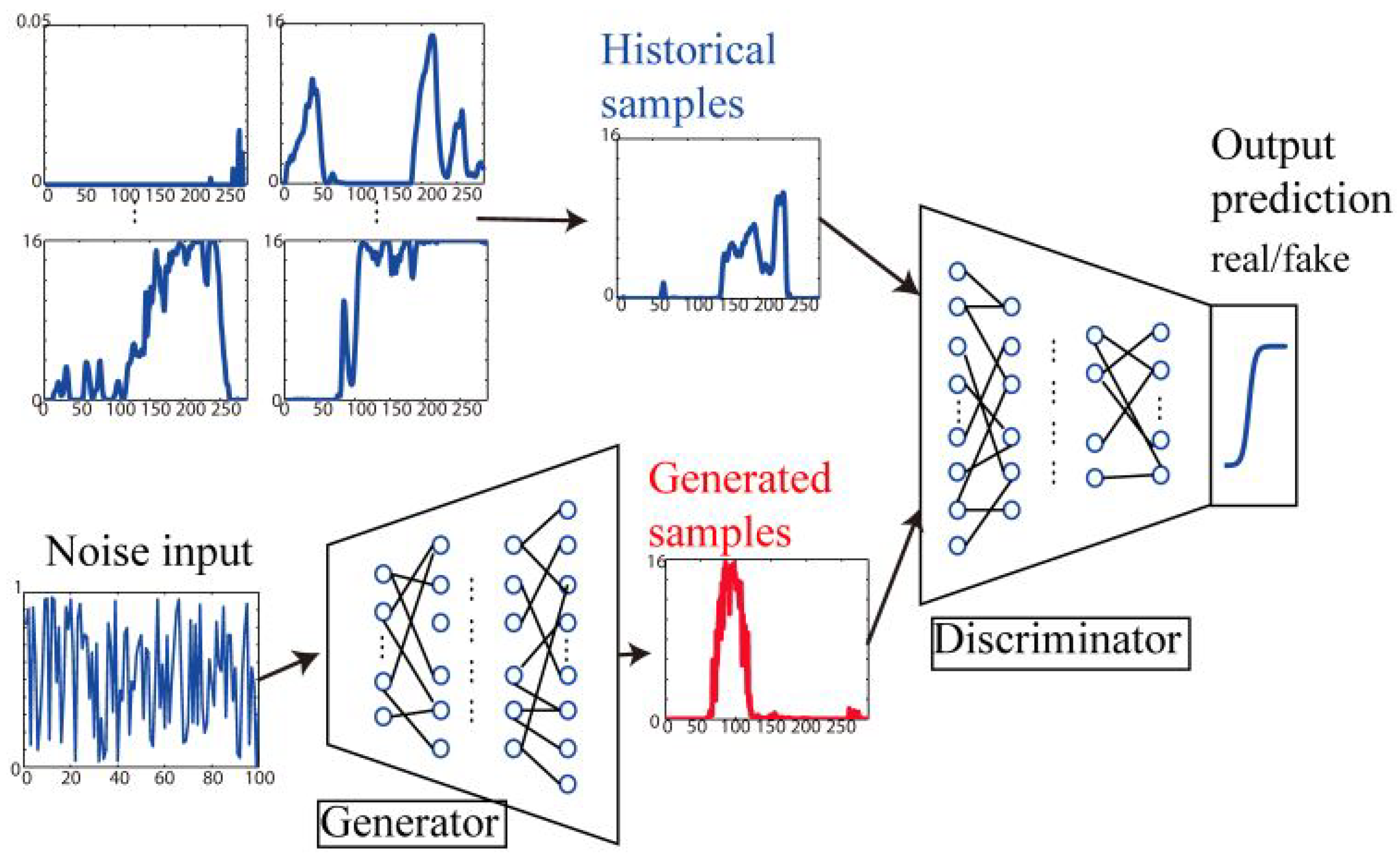
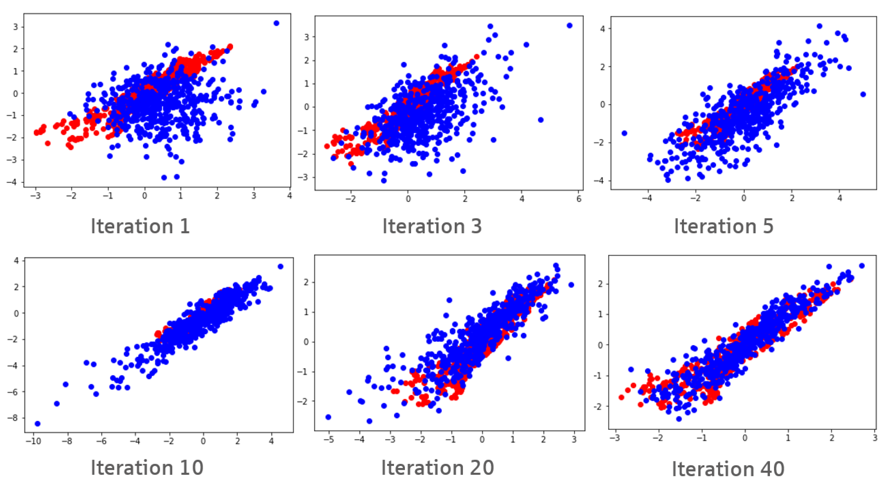
2.3. Generative Adversarial Networks

Generative adversarial networks, called GANs, are an architecture consisting of two neural networks that are interacting with each other. In 2014, GANs were introduced by Goodfellow et al. (2014) and have gained much attention afterwards because of their promising results, especially in image generation. A good introduction to GANs can be found in Goodfellow et al. (2014), Goodfellow (2016) and Chollet (2018). According to Motwani and Parmar (2020) and Li et al. (2020), GANs are one of the dominant methods for the generation of realistic and diverse examples in the domains of computer vision, image generation, image style transfer, text-to-image-translations, time-series synthesis, natural language processing, etc.
Other popular methods for the generation of data based on empirical observations are variational autoencoders and fully visible belief networks; see Goodfellow (2016, p. 14).
Technically, a GAN consists of two neural networks, named generator and discriminator. The discriminator network is trained to distinguish real data points from “fake” data points and assigns every given data point a probability of this data point being real. The input to the generator network is random noise stemming from a so-called latent space. The generator is trained to produce data points that look like real data points and would be classified by the discriminator as being real with a high probability. Figure 2 illustrates the general architecture of GANs’ training procedure.
Formally, we can define GANs as follows; see Goodfellow et al. (2014, Chapter 3) and Wiese et al. (2020, Chapter 4). For this purpose, let ( Ω , F , P ) be a probability space and N X , N Z N . Furthermore, assume that X and Z are R N X and R N Z valued random variables, respectively. Random variable Z represents the latent random noise variable, and X represents the targeted random variable. ( R N Z , B ( R N Z ) ) is called the latent space. Usually, N Z > N X is chosen; see Goodfellow (2016, p. 18). The goal of the GAN is to train a generator network, such that the generator mapping of the random variable Z to R N X has the same distribution as target variable X. Let us first define the generator formally.
Definition 2.
Let G θ G : R N Z R N X be a neural network with parameter space Θ G and θ G Θ G . Random variable X ˜ = G θ G ( Z ) is called the generated random variable. Network G θ G is called the generator.
The counterpart of the generator in this game is the discriminator that assigns to each generated or real data point x R N X a probability of being a realization of the target distribution.
Definition 3.
A neural network with D θ D : R N X [ 0 , 1 ] with parameter space Θ D and θ D Θ D is called a discriminator.
Given these two neural networks, we can now define a GAN as in Goodfellow (2016, Chapter 3):
Definition 4.
A GAN (generative adversarial network) is a network consisting of discriminator D θ D and generator G θ G . The parameters θ D Θ D and θ G Θ G of both networks are trained to optimize the value function:
V ( G θ G , D θ D ) = E [ log ( D θ D ( X ) ) ] + E [ log ( 1 D θ D ( G θ G ( Z ) ) ]
with X denoting the targeted random variable, and Z denoting the latent random noise variable.
Z can be sampled from the latent space with a any chosen distribution; however, one usually uses normal distribution for Z; see Chollet (2018, Chapter 8.5.2). Value function V has been defined in Goodfellow (2016). Where does it come from? Discriminator D θ D has to distinguish between real and fake samples, i.e., to solve a binary classification problem; see Goodfellow (2016, Chapter 3.2). The discrete version of value function V corresponds to the binary cross entropy loss for the discriminator, which is usually used for binary classification issues solved by neural networks. A definition of the binary cross entropy loss can be found in, e.g., Ho and Wookey (2019, Section 3).
The optimization (the GAN objective) is given by
min θ G Θ G max θ D Θ D V ( G θ G , D θ D ) .
The above means that the discriminator is optimized to distinguish real samples from generated samples, whereas the generator tries to “fool” the discriminator by generating such good samples that the discriminator is not able to distinguish them from real ones. A detailed derivation of the optimization of the objective and the modifications that can be used in GAN training are found in Goodfellow (2016, p. 22) and Wiese et al. (2020, p. 9).
In the inner loop, V ( G θ G , D θ D ) takes its maximum value if the discriminator correctly assigns a value of 1 for all “real” data points and a value of 0 to all generated data points. The parameters of the discriminator network θ D are optimized to fulfill this task. In the outer loop, the generator tries to fool the discriminator and its parameters, θ G , are optimized to maximize D θ D ( G θ G ( Z ) ) , meaning that the discriminator shall assign a high probability of being real to “fake” data points. To achieve the optimization of the value function, in practice, the training alternates between k steps of optimizing D θ D and one step of optimizing G θ G . k is one of the hyperparameters of the GAN. The starting point of the parameters of the neural networks D θ D and G θ G is given by random initialization.
An algorithm for GAN training can be found in Goodfellow et al. (2014, Chapter 4, Algorithm 1). In every iteration of the training process, the two neural networks are trained in turns, while parameters of the other network are fixed. We provide here a short version of this algorithm.
Algorithm 1 Algorithm for GAN training with SGD (stochastic gradient descent) as an optimizer; see Goodfellow et al. (2014, Chapter 4, Algorithm 1)
The discriminator is trained k times more often than the generator, the dimension of the latent space Z is N Z , M N is the batch size. All are hyperparameters of the GAN.
The learning rates of the SGD algorithm are γ D and γ G .
  • Initialize parameters w for discriminator and θ for generator.
  • For each optimization step of the SGD:
    -
    for k steps do
    *
    Randomly draw sample batch { x 1 , , x M } of size M from data generating distribution
    *
    Randomly sample { z 1 , , z M } independent realizations of random variable Z
    *
    Update the parameters w of the discriminator (with fixed parameters θ of the generator):
    w n e u = w a l t + γ D w 1 M i = 1 M log ( D w ( x i ) + log 1 D w ( G θ ( z i ) .
    -
    Randomly sample { z 1 , , z M } independent realizations of random variable Z
    -
    Update the parameters θ of the generator (with fixed parameters w of the discriminator)
    θ n e u = θ a l t γ G θ 1 M i = 1 M log 1 D w ( G θ ( z i ) .
Despite their success, GANs remain difficult to train, as stated, e.g., in Motwani and Parmar (2020). The largest issue with GANs according to Goodfellow (2016, p. 34) is the non-convergence often observed in practice. This is due a GAN not being a normal optimization task but a dynamic system that seeks for an equilibrium between two forces; see Chollet (2018, Chapter 8.5.2) and Salimans et al. (2016, p. 2). Each time any parameter of one component, either discriminator or the generator, is modified, it results in the instability of this dynamic system; see Motwani and Parmar (2020, p. 2). Mazumdar et al. (2020, p. 25) provide a mathematical analysis of this non-convergence issue and state that “first, the equilibrium [of the GAN] that is sought is generally a saddle point and second, the dynamics of GANs are complex enough to admit limit cycles”.
Therefore, the model architecture and the hyperparameter have to be chosen carefully. Unfortunately, at the moment, there is no way to tell which hyperparameters and which architecture will perform best in during training; see Motwani and Parmar (2020, p. 2). Therefore, some form of validation has to be performed to control the convergence of the GAN. One possible validation measure is the Wasserstein distance; see Section 4.3.
The evolution of the quality of the output during training can be visualized in the case of a two-dimensional data distribution in Figure 3. The red data here represent the empirical data to be learned, whereas blue data are generated at the current stage of training of the generator. For the illustration, we here use the same amount of red and blue dots in each figure. One can clearly see that the generated data match the empirical data more closely when more training iterations of the GAN have taken place.

3. Results of a GAN-Based Internal Model

3.1. Workflow of a GAN-Based Internal Model

The strength of GANs is particularly what ESGs should be good at—producing samples of an unknown distribution based on empirical examples of that distribution. Therefore, we will apply a GAN as an ESG.
This is a different task from re-sampling, as explained, e.g., in Yu (2002, pp. 3–7), where the task is to use subsets or bootstrapping from the empirical data to derive data sets with the same statistical properties as the empirical data. As we only have about 20 years of financial market history and need to evaluate a 0.5% percentile, i.e., a 1-in-200 years event, we need to produce financial data that have not yet occurred in the financial market but could have. Therefore, re-sampling is not an option. The dependency modelling in a GAN-based ESG is similar to using an empirical copula for the risk factors in a classical ESG based on the Monte-Carlo technique.
Figure 4 shows that a GAN in contrast to resampling really generates new scenarios. In this figure, we show scatterplots of four different risk factor pairs: 5-year interest rates vs. 10-year interest rates, Eurostoxx50 vs. German government bond spreads, Italian vs. German government bond spreads and AAA corporate credit spreads vs. BBB corporate credit spreads. Details to the data can be found in Section 4.1 and Section 4.2.
The orange dots in the figure represent the 50,000 scenarios generated by the GAN for these risk factors. The blue dots are the 4330 empirical data points used for GAN training. The structure of the orange dots mimics the structure of the blue dots but also generates new results that are not found within the blue dots. In resampling, the data would not go beyond the boundaries of the blue dots.
For all 50,000 generated 46-dimensional scenario data points, we calculated the euclidian distance to the nearest empirical data point in the 46-dimensional space. This distance is always above 0 and varies between 0.3 and 5.7. Figure 5 shows the histogramm of those 50,000 minimum distances. In re-sampling procedures, the distance between generated and empiric data points always equals 0. This illustrates that the GAN really generates new scenarios.
As shown in Chen et al. (2018), a GAN can be used to create new and distinct scenarios that capture the intrinsic features of the historical data. Fu et al. (2019, p. 3) already noted in their paper that a GAN, as a non-parametric method, can be applied to learn the correlation and volatility structures of the historical time series data and produce unlimited real-like samples that have the same characteristics as the empirical observed time-series. Fu et al. (2019, Chapter 5) tested this with two stocks and calculated a 1-day VaR.
In our study here, we demonstrate how to expand this to an entire internal model—with enough risk factors to model the full band-width of investments for an insurance company and for a one year time horizon as required in Solvency 2.
Figure 6 illustrates schematically the workflow of a GAN-based internal model. It follows the process of a classical internal model (see Bennemann (2011, p. 177 cont.) and Gründl et al. (2019, p. 82)), except that the ESG step is replaced by a GAN instead of a Monte-Carlo simulation. Details to the steps are provided in Section 4 and are similar to the steps taken in Wiese et al. (2020, Chapter 6). Methodology and data used are explained there, as well.

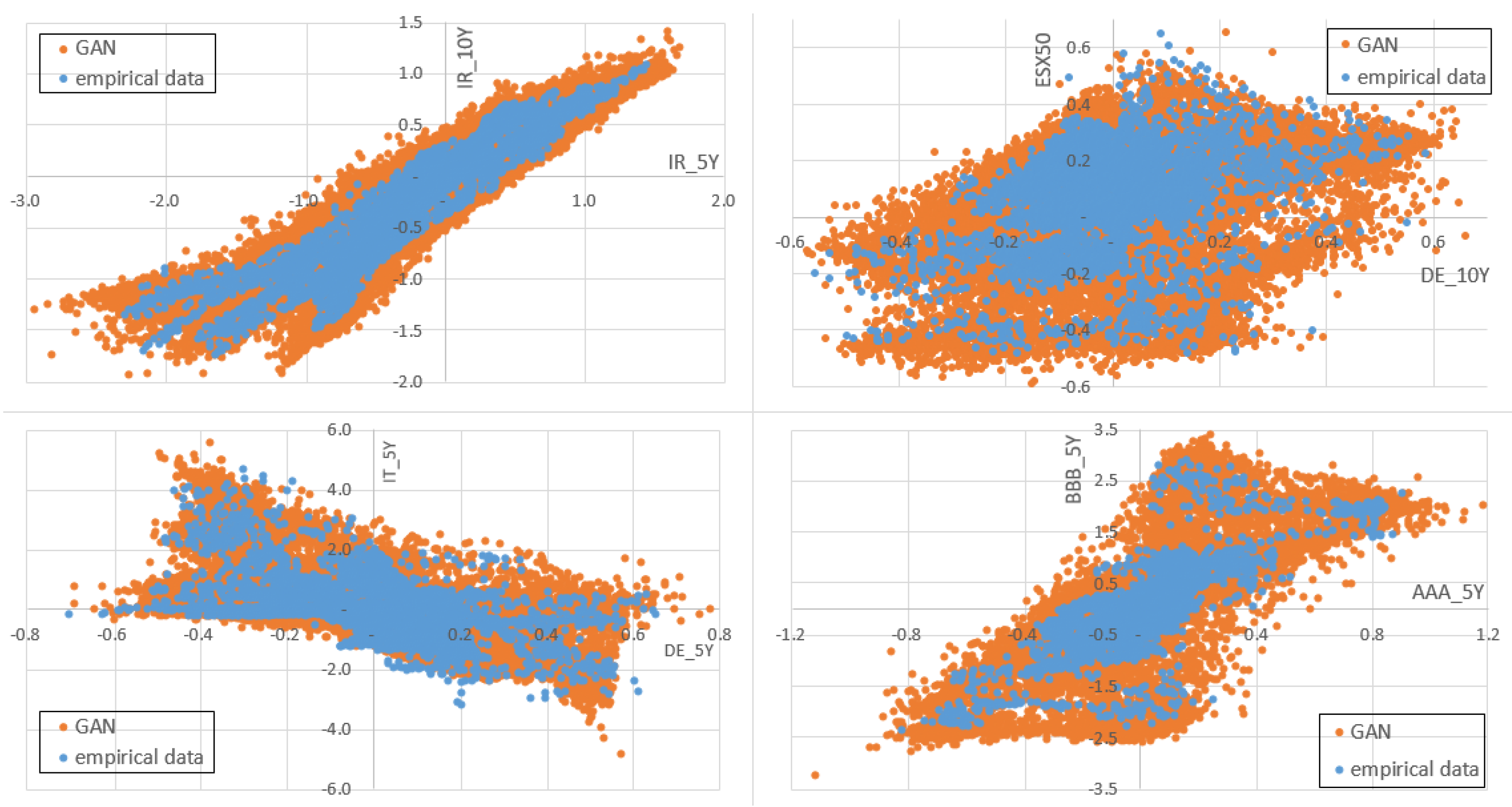
3.2. Comparison of GAN Results with the Results of the MCRCS Study

When having implemented a GAN-based model as explained in Section 4, we can compare the results of our GAN-based model for both risk factors and benchmarking portfolios with the risk derived from approved internal models in Europe using the results of the MCRCS study. The study for year-end 2019 can be found on EIOPA’s homepage; see EIOPA (2021a).
The results on risk factor basis are analyzed based on the shocks generated or implied by the ESGs in the study in Section 3.3. A shock hereby is defined in EIOPA (2021a, p. 11) as
Definition 5.
A shock is the absolute change of a risk factor over a one-year time horizon. Depending on the type of risk factor, the shocks can either be two-sided (e.g., interest rates “up/down”) or one-sided (e.g., credit spreads “up”). This metric takes into account the undertakings’ individual risk measure definitions and is based on the 0.5% and 99.5% quantiles for two-sided risk factors and the 99.5% quantile for one-sided risk factors, respectively.
The main comparison between the results for the benchmark portfolios is based on the risk charge, which is defined in EIOPA MCRCS Project Group (2020b, Section 2). We analyze this in Section 3.4.
Definition 6.
The risk charge is the ratio of the modeled Value at Risk (99.5%, one year horizon) and the provided market value of the portfolio.
The results are presented in diagrams, showing the 10%, 25%, 75% and 90%-percentile of all insurance companies participating in the study. There are 21 participants and only insurances having at least some exposure in this risk factor are shown. For our comparison here, we want to compare our results with the entire bandwidth of internal models in Europe. Therefore, we calculated an implied mean and standard deviation based on the 10% and 90% percentile under the assumption of a normal distribution of results. Based on this, we derived a theoretical 1% and 99% percentile to show as boxes for each maturity/sub-type of the risk factors resp. portfolios. The given 10%- and 90%-percentile are shown as frames inside the boxes.
We enrich those MCRCS results with a blue dot representing the shock resp. risk charge for that risk factor or portfolio generated by our GAN-based model.
After that, in Section 3.5, we use the results shown in a so-called excursus focusing on the market development in the COVID-19 crisis to compare results of the approved models with our GAN-based model as well. The dependency structures of the internal models are analyzed using joint quantile exceedance as a metric in EIOPA (2021a, Chapter 5.2.6). The comparison to the GAN results can be found in Section 3.6. The Section concludes with an examination of the stability of the GAN output.

3.3. Comparison on Risk-Factor Level

In this study, we will show the comparison of the five most important risk factor categories (corporate and sovereign credit spread, equity and up-and-down interest rate). Other risk factors show a similar behaviour.
For corporate as well as sovereign credit spreads in Figure 7, we see a very good alignment between the GAN-based model and the approved internal models. The comparison of the Ireland sovereign spread has been excluded from the comparison as only five participants submitted results for this risk factor. The shock reported in EIOPA (2021a, p. 26) varies between 1.1% and 3.5%, which seems inconsistent to the sharp increase of up to 8.3% within 12 months that Ireland experienced during financial crisis. Therefore, data quality here seems not to be sufficient for a comparison.
On the equity side in Figure 8, the shifts are also similar for most of the risk factors. For the FTSE100, the GAN produces less severe shocks than most of the other models. This behaviour, however, can actually be found in the training data as the FTSE100 is less volatile than the other indices for the time frame used in GAN training. Thus, the GAN here produces plausible results.
For interest rates, however, the picture is a bit more complex, as Figure 9 illustrates.
The up-shifts generated by the GAN-based model are within the boxes for all buckets. However, for longer maturities, the shifts tend to be at the lower end of the boxes. This effect is due to the time span of the data used for the training of the GAN where interest rates are mostly decreasing.
For down-shifts, we can observe the following behaviour: Short-term interest rates are below the boxes, whereas the middle and longer term interest rates are inside the boxes. This can be explained by the interest rate’s development: The time span used for training of the GAN shows a sharp decrease in interest rates, especially in the short-term, whereas longer-term interest rates behaved more stable. This behaviour is mimicked by the GAN. In traditional ESGs, additionally to the longer time span used for calibration, often expert judgement by the insurers leads to a lower bound on how negative interest rates can become. One of the most common arguments for a lower bound of interest rates according to Grasselli and Lipton (2019, Chapter 4) is the fact that instead of investing money with negative interest rates, asset managers could also convert the money into cash and store this. However, the conversion of large amounts of money into cash poses many issues and is, therefore, unrealistic. Grasselli and Lipton (2019) use this argument to derive a cash-related physical lower bound of about −0.5%. Danthine (2017, Chapter 2) states that the lower boundary for interest rates is not far below −0.75% in the current environment. For illustration purposes, we introduced light blue dots in Figure 9 where we limited the downshift to −1.9% in the GAN (as this is the value of the 10%-percentile). This, however, does not change the results on the portfolio level, as presented in Section 3.4, significantly (difference in VaR is always below 0.1%). If an insurance company wishes to limit downside interest rate shifts, this would be a reasonable approach.

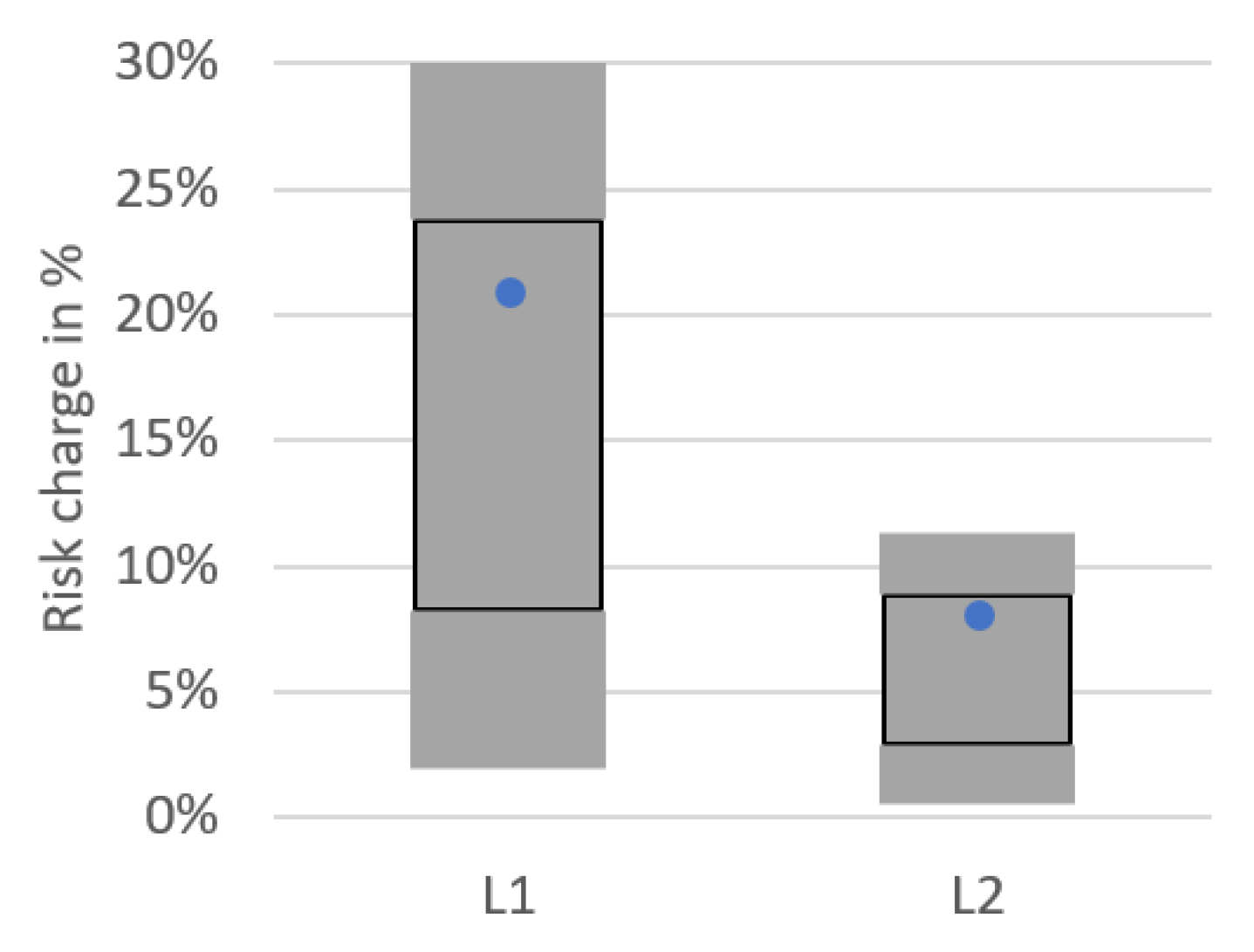
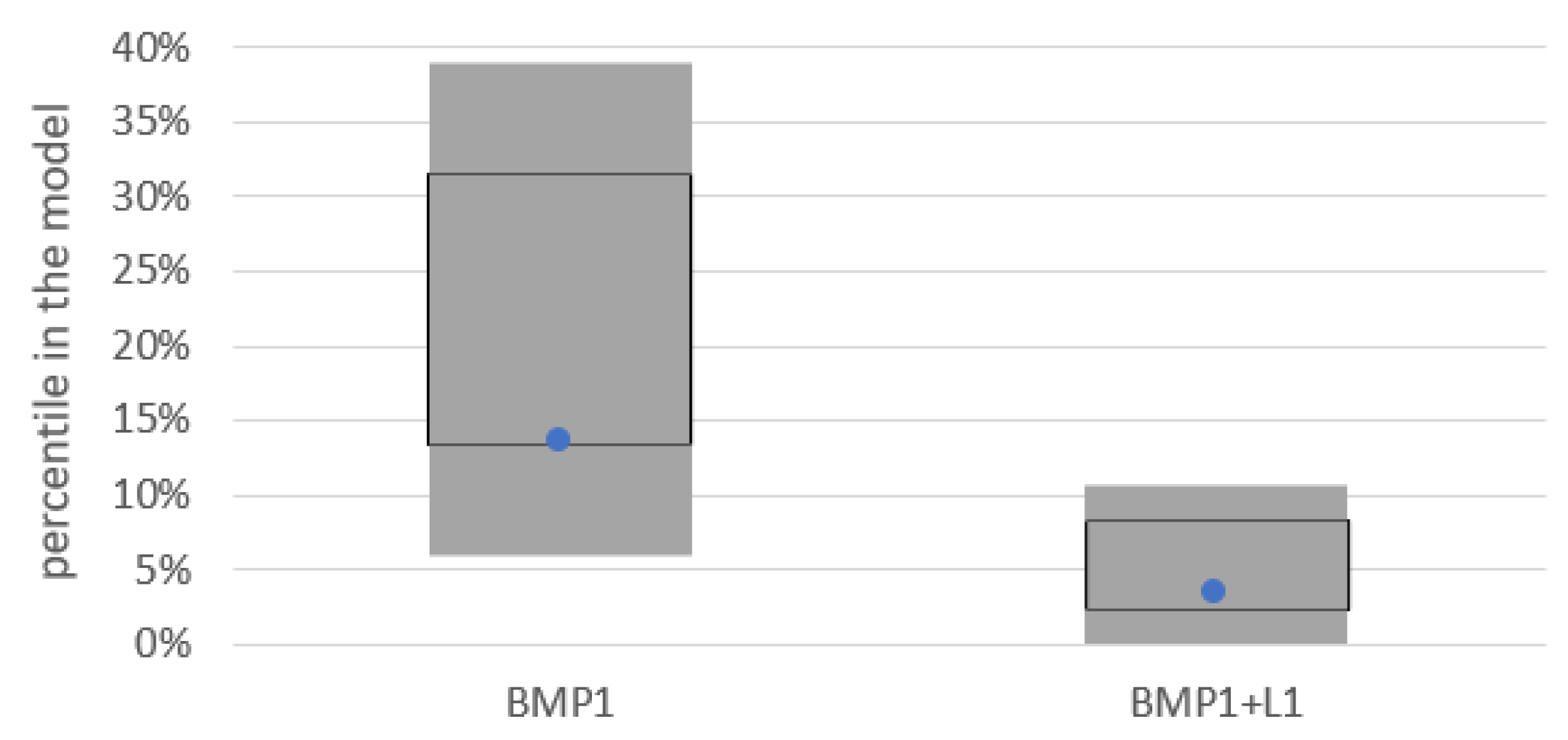
3.4. Comparison on the Portfolio Level

First, in Figure 10, we show the comparison of the risk charges for the ten asset-only benchmark portfolio of the MCRCS study:
The risk charge of the GAN-based model fits well to the risk charges of the established models and always lays within the gray boxes. The blue dot tends to be at the lower part of the boxes for the portfolios. This is due to the fact that increasing interest rates form a main risk. As we showed in Section 3.3, the shocks for the GAN-based model for increasing interest rates are at the lower part of the boxes for longer maturities as well. Thus, this behaviour can be explained.
The two liability-only portfolios as seen in Figure 11 differ by durations: L1 has a duration of 13.1 years versus a 4.6 years duration of L2.
For the liability-only portfolios as well, the risk charge of the GAN-based model fits well to the risk charges of the established models and always falls within the gray boxes. The blue dot tends to be at the upper part of the boxes for the portfolios. The risk charge of the liability-only portfolios is caused by scenarios with decreasing interest rates. In the risk factor comparison of the interest rate down shock in Section 3.3, the interest rate down-shifts tend to be more severe for most maturities for the GAN-based model than for the average of the other models. Therefore, it seems plausible for the resulting portfolio risk to be at the upper part as well.
Figure 12 displays the risk charge for each of the combined asset-liability benchmark portfolios, which comprises portfolios with the longer (left) and shorter liability structure (right).
For the combined portfolios as well, the GAN-based model shows comparable results to the established models.

3.5. Comparison of the COVID-19 Backtesting Results

In a so-called excursus, EIOPA (2021a, pp. 17–21), the study examines whether the turmoil in the financial markets following the COVID-19 crisis in spring 2020 is part of the generated scenarios of the tested models. This could be seen as a form of backtesting exercise as this event was not part of the calibration/training process for the ESGs. In the study, EIOPA calculates for each benchmark portfolio P the worst case one-year rolling return, including the COVID-19 crisis:
W o r s t C a s e ( P ) = min t T M a r k e t V a l u e ( P ) t M a r k e t V a l u e ( P ) t 258 1 ,
where
T = Last working day for each month in the period 31.01.2017 30.09.2020 .
Let F P , M be the empirical distribution function under model M for the relative returns of portfolio P with respect to the 50,000 scenarios relative to the current market value. By
α P , M = F P , M W o r s t C a s e ( P )
we denote the probability that a relative loss that is as least as severe as the COVID-19 crisis occurs to portfolio P under model M.
EIOPA (2021a, p. 21) states that “the COVID-19 related market impacts can certainly be seen as significant. From a general perspective of internal market risk models, there is no evidence that this could be interpreted as an event beyond the scope of application of these models.” This means that the worst-case losses in this time period considered for every benchmark portfolio should be within the loss distribution generated by the models and ideally α P , M is above 0.5%. The worst case for most portfolios occurs during COVID-19-related market turmoil in the first half of 2020; see EIOPA (2021a, p. 19).
An explicit comparison of values α P , M for the models is only provided for the asset-only benchmark portfolio BMP1 and the asset-liability benchmark portfolio BMP1+L1, see Figure 13. As in Section 3.3 and Section 3.4 above, the same meaning of the boxes apply in the graph.
The results match with the results of Section 3.4. One can state that the GAN-based model in this examination behaves similarly to the other models. For other benchmark portfolios, we also calculate the implied percentiles of the WorstCase return in spring 2020 and the corresponding value α P , G A N for the GAN-based model α P , G A N . In Table 1, for portfolio BMP1+L1, a value of α P , G A N = 3.5 % means that in 3.5 % of the scenarios, the GAN-based model generated a return that is more severe than 58.2 % , with 58.2 % being the WorstCase return of portfolio BMP1+L1 encountered during the COVID-19 crisis.
As displayed in Table 1, for all portfolios, α P , G A N for the GAN-based model is above 0.5%, which is in line with the EIOPA expectations mentioned above.

3.6. Comparison of Joint Quantile Exceedance Results

The market-risk dependency structures in the models are examined in EIOPA (2021a, Chapter 5.2.6) on a risk factor basis. Results are only presented for the comparison of joint quantile exceedance, which is defined as follows.
Definition 7.
The bivariate Joint Quantile Exceedance probability (JQE) is the joint probability that both risk factors will simultaneously surpass the same quantile.
For the comparison, a percentile of 80% is used. This is a compromise that not only provides enough data for examination but also for focusing on the tail of the distribution. For independent risk factors, the joint quantile exceedance, therefore, equals J Q E = 20 % · 20 % = 4 % . If risk factors have a correlation of 1, JQE equals 20 % ; for a correlation of −1, JQE is 0 % . In the study, EIOPA (2021a, p. 34), the matrix of JQEs is presented as boxplots for all pairs of seven selected risk factors. Please note that the joint quantile exceedance of the risk factor with itself is not shown.
We show in Figure 14 the results of the comparison for one credit spread, one equity and one interest rate risk factor. Other comparisons follow a similar pattern.
For pairwise JQE results, the GAN-based model always lays within boxes of the internal models of the MCRCS study. Therefore, the dependency structure generated by the GAN-based ESG seems to resemble the dependency structures used in internal market risk models in Europe.

3.7. Stability of GAN Results

One important question for an internal model is how stable the results of the GAN-based ESG are. Since the GAN is initialized with random parameters and the sampling for the batches in training is random as well as the generation of the random variables in latent space, we want to test whether the results in the previous sections are stable for different GAN runs.
We trained four different GANs with the same architecture (but with different random initialization) and used each of those four trained generators to generate 50,000 scenarios five times for each of the 46 risk factors, leading to 20 sets of 50,000 scenarios each. For these 20 sets, we now check how stable the resulting risk charge for the risk factors is, particularly whether the shift (up and down) in each of the sets is within the gray boxes from the EIOPA MCRCS study used above.
Figure 15 illustrates this for four different risk factors, namely 5-year interest rate up- and down-shift, 5-year corporate credit spreads AA and 5-year German sovereign credit spreads. For interest rate down shifts, we display absolute values in the graph. We here present the gray boxes from MCRCS study as above, but instead of one blue dot for the GAN result, we show here 20 coloured dots—each dot representing one of the 20 different runs. As the dots overlap each other, not all dots can be seen in this graph.
For all risk factors, even those that are not shown in the figure, we analyzed that all shifts are within the gray boxes for each of the 20 runs, except for the outliers in interest rates as commented on in Section 3.3.
For a quantitative stability check, we first calculate for each of the 46 risk factors in each of the 20 scenario sets, the 0.5-percentile and the 99.5-percentile (equalling the up- and down shift used in MCRCS study). Then, for each risk factor and each percentile, we compute the empirical first and third quartiles Q1 and Q3 over the 20 runs and report the coefficient of quartile variation by using the following.
CQV = Q 3 Q 1 Q 3 + Q 1 ,
See Kokoska and Zwillinger (2000, Equation (2.30)). Appendix A shows the entire table of the results for all risk factors and both percentiles. We can state that the coefficient of quartile variation for both percentiles differs between 0.5% and 10.0%. This indicates that the results are stable over different runs of the GAN.
Overall, the GAN-based model shows, in every dimension in the study, comparable results to the certified internal models in Europe. Therefore, the proof of concept of whether a GAN can serve as an ESG for market risk modeling is successful. Please note that from a regulatory perspective, it is desirable that all approved internal models for market risk lead to comparable results. Therefore, this research indicates that a GAN-based model can be seen as an appropriate alternative method of market risk modeling.

4. Methodology and Data

4.1. Data Selection

For the purpose of this article, we choose to model the risk charge for the ten MCRCS asset-only benchmark portfolios, the two liability-only portfolios and for the ten combined asset-liability portfolios. We are particularly interested in the ability of the GAN to generate the joint movement of the risk factors and not the distribution of single instruments. Therefore, we want to simulate only instruments and risk factors that are needed in the benchmark portfolios.
Out of the 104 instruments in the MCRCS study, only 71 are included in the benchmark portfolios; 33 single instruments are left out in our model. To model those instruments, we have to select financial time series for the relevant risk factors (i.e., equity index and interest rate buckets) as most of the instruments itself are not traded and, therefore, have no time series. We found 46 risk factors to be sufficient for evaluating those instruments because several instruments depend on the same risk factor.
All relevant financial data will be derived from Bloomberg. An aggregated view of these risk factors together with the Bloomberg sources (“ticker”) can be found in Appendix A. A mapping table indicating for each of the 71 instruments which risk factors are used for calculation can be found in Appendix B. In the same appendix, comments on any approximations used are found as well.
EUR swap rates and EUR corporate yields are available on a daily basis in Bloomberg since 25 Feb 2002 resp. 28 Mar 2002. Since the study is conducted at year-end 2019, we take the datapool from the end of March 2002 to December 2019 as the basis of our GAN training. Therefore, we used 4588 daily observations, which covers almost 18 years of 46 time series to train the GAN.

4.2. Data Preparation

For Solvency 2, we need to model the market risk with a time horizon of one year, but we have daily observations. According to Yoon et al. (2019, p. 1) this temporal setting poses a particular challenge to generative modeling. One solution is to use the daily data to train the GAN model and then use some autocorrelation function to generate an annual time series based on daily returns; see Fu et al. (2019) and Deutsch (2004, Chapter 34). However, an autoregressive model can only be used if strong assumptions about the underlying processes are made.
Another solution is to use overlapping rolling windows of annual returns on a daily basis to train the model. We decide to calculate the returns in rolling annual time windows for all available days. This method is, e.g., used in Wiese et al. (2020, p. 16) and also in EIOPA (2021a, p. 17). Deutsch (2004) describes the procedure in Section 32.3. He explains the drawback that the generated annual returns have a high autocorrelation as they only differ in one daily return. However, we will make the assumption that each of these one-year returns is one possible scenario with respect to how risk factors can shift within one year even if this implies that input data are not independent anymore. This, however, is similar to classical ESGs where for calibration purposes rolling windows are often used as there are not enough data available to use disjoint annual return data.
The second decision to be made is how to calculate returns. Returns can be calculated either as a simple difference of the two time points in question; alternatively, one can calculate relative returns, log-returns are often used or one can use other transformations. EIOPA (2021a) uses simple differences for interest rates and credit spreads and relative returns for equities, real estate and foreign exchange. The reasoning behind this is that in the low interest rate environment, relative returns do not make sense in many cases. Therefore, we will stick with this scheme.
To calculate rolling one-year returns, we make the assumption that one year has 258 trading days. This is obtained by dividing the number of daily data we have for the risk factors (T = 4588 observations) by the number of years from which the data originate (17.8 years).
This means that, for each risk factor with a value of s t at time t 1 , , T 258 with t being the number of days in the data set, the rolling annual-return is calculated as follows:
r t = s t + 258 s t 1 , t = 1 , , T 258 .
For interest rates and credit spreads, however, we calculate absolute rolling returns as follows.
r t = s t + 258 s t , t = 1 , , T 258 .
Therefore, the training data for the GAN comprises T 258 = 4330 observations of annual returns for each of the 46 risk factors.
A neural network does not work properly when the input data are at different scales; see Chollet (2018, Chapter 3.6.2). Therefore, we will normalize the return data r t by risk factor (dividing by standard deviation, adjusting by the mean). As with GANs, there is no split of the data into a training/test/validation data sets, so we can use all the data for training; see Goodfellow (2016, Chapter 3).

4.3. Implementation of a GAN-Based ESG

We implement the GAN in programming language Python, which has many packages that are useful in data science contexts. For pre- and post-processing, we use the packages pandas, numpy, scipy and matplotlib. Our GAN implementation itself is based on the package keras, as described in Chollet (2018, Chapter 8.5).
It runs in a cloud with 144 virtual CPUs and 48 GiB RAM on a third-generation Intel Xeon processor. The training time for this GAN is about half an hour; the generation of the 50,000 scenarios as outputs takes less than one minute. We used the following configuration for the GAN-based ESG:
  • 4 layers for discriminator and generator;
  • 400 neurons per layer in the discriminator and 200 in the generator;
  • k = 10 training iterations for the generator in each discriminator training;
  • Batch size is M = 200 ;
  • Dimension of the latent space is 200, and the distribution of Z is a multivariate normal with mean = 0 and std = 0.02 ;
  • Initialization of the generator and discriminator using multivariate normal distribution with mean = 0 and std = 0.02 ;
  • We use LeakyReLu as activation functions except for the output layers, which use sigmoid (for discriminator) and linear (for generator) activation functions. We use the Adam optimizer and regulation technique batch normalization after each hidden layer in the network. The loss function is binary crossentropy.
LeakyRelu hereby is an alternative to the popular activation function Relu and is defined as follows.
g ( x ) = x x > 0 α x x < 0
In our implementation, we set α = 0.2 .
The adam optimizer is used here instead of the SGD; see Algorithmus 1. The adam optimizer uses the following algorithm to update the weights to w k + 1 given w k in the generator and discriminator networks:
v k = β 2 v k 1 + ( 1 β 2 ) g k g k , k = 1 , 2 m k = β 1 m k 1 + ( 1 β 1 ) g k , k = 1 , 2 w k + 1 = w k + γ k 1 β 2 k + 1 1 β 1 k + 1 m k 1 v k + δ , k = 0 , 1 ,
with v 0 und m 0 being null vectors and ⊙ the Hadamard product.
The following parameters are used in our implementation.
γ 0 = γ 2 = = 0.0002 β 1 = 0.5 β 2 = 0.999 δ = 10 7
Definitions and explanations for these functions and terms can be found in, e.g., Viehmann (2019) and Chollet (2018).
According to Goodfellow (2016, Chapter 5.2), “it is not clear how to quantitatively evaluate generative models. Models that obtain good likelihood can generate bad samples, and models that generate good samples can have poor likelihood. There is no clearly justified way to quantitatively score samples”. According to Theis et al. (2015, p. 1), “generative models need to be evaluated directly with respect to the application(s) they were intended for”.
In the literature, where scenario generation for financial or similar data is performed by GANs or other generative models, there is no clear favorite measure used for the validation of the results. Many papers focus on the visual inspection of histograms, scatterplots, etc., together with a comparison of some basic statistics (mean, standard deviation, skewness, kurtosis, percentiles and autocorrelation). Examples for this evaluation method include the following papers: Franco-Pedroso et al. (2019), Henry-Labordere (2019), Lezmi et al. (2020), Fu et al. (2019), Chen et al. (2018) and Marti (2020).
As for internal models, the marginal distribution of the risk factors are of great importance, we will use Wasserstein distance in this paper to evaluate whether the generated data match the empirical data. Wasserstein distance is commonly used to calculate the distance between two probability distribution functions, as mentioned in Borji (2019) and Wiese et al. (2020). The definition of the Wasserstein distance can be found, e.g., in Hallin et al. (2021, p. 5). We use here the univariate Wasserstein distance with p = 1 as defined in Hallin et al. (2021, Equation (1)).
Definition 8.
For univariate distributions P and Q with distribution functions F and G, the p-Wasserstein distance is given by the L p -distance.
W p ( P , Q ) = 0 1 | F 1 ( t ) G 1 ( t ) | p d t 1 / p .
One could alternatively use other metrics to measure the distance between two probability distribution functions, e.g., Kullback–Leibler divergence. We decided for the Wasserstein distance as it is easily interpretable, implementable and often used in the machine learning context.
Figure 16 shows the development of Wasserstein distances between the empirical distribution functions of the training and the generated data for all 46 risk factors in our GAN. We can see in this graph that the Wasserstein distance for all risk factors decreases over the training iterations in this configuration.
To arrive at the GAN architecture mentioned above, we trained 25 different GANs varying in the number of layers and the number of neurons per layer. For each of the 25 configurations, we then calculated the maximum of the Wasserstein distances over all risk factors. We then compared the minimum of this maximal Wasserstein distance over the training iterations between the 25 configurations and choose the configuration possessing the lowest value. Details and results of this procedure can be found in Appendix C.
We now use the trained generator with this configuration to generate 50,000 financial scenarios for all risk factors.

4.4. Valuation of Financial Instruments and Portfolio Aggregation

As mentioned before, we want to evaluate the benchmark portfolios of the MCRCS study, which comprise 71 instruments. Thus, first, we have to evaluate the instruments in each scenario by applying the generated data for the 46 risk factors. For this task, we use the following formulas and methods.
(1). 
Zero-coupon bond valuation
All interest- and spread-related instruments are zero-coupon bonds and can be valued with present value discounting for scenario n = 1 , , 50,000 as follows:
Z C ( r τ 0 , r τ n , s τ 0 , s τ n , τ ) = 1 ( 1 + r τ 0 + r τ n + s τ 0 + s τ n ) τ
where Z C means the value of a zero-coupon bond with maturity τ with the starting interest rate being r τ 0 and the shift in scenario n being r τ n and the starting spread being s τ 0 and the shift in scenario n of the spread being s τ n . τ hereby equals the maturity of the bond, as found in Table A2 in Appendix B. The starting time for MCRCS study is year-end 2019. For details on the valuation of zero coupon bonds, we refer to Albrecht and Maurer (2016, Chapter 8.4).
For the default and migration process of corporate bonds, we use the rating migration matrix from Ratings (2018). This is the S&P average European 1-year corporate transition rate for the years 1981–2018, where we assume that high yield bonds are B-rated. Since the credit spread can be interpreted as the probability of a bond defaulting, we scale the downgrade probabilities in the scenarios according to the percentage the generated spread is above the starting spread. For sovereign bonds, we analogously assumed a default according to the rating of the country, scaled using the same methodology as for corporate bonds. The recovery rate is set at 45%.
(2). 
Equity and property instrument valuation
For equities and property, the market value of the instruments in the scenarios is scaled with the percental shift of the respective risk factor to evaluate instruments in scenario n.
(3). 
Valuation of the liabilities
The method used for discounting of the liabilities in Solvency 2 is laid out in EIOPA (2019). The Solvency 2 framework assumes that liquidity in the interest rate market can only be assumed up to a maturity of 20 years. In this period, a credit risk adjustment of 10 basispoints is deducted before discounting. Afterwards, the yield curve is extrapolated to a so-called ultimate forward rate (abbr. “UFR”), which is the 1-year forward rate to be valid at a maturity of 60 years. The UFR is updated on an annual basis and at year-end 2019 was 3.9%. The extrapolation method is based on Smith and Wilson (2001), and its features are discussed, e.g., in Viehmann (2019) and Lagerås and Lindholm (2016). In our implementation, after generating the scenarios, we use this extrapolation method to derive the risk-free yield curve and discount the two liability benchmark portfolios accordingly.
(4). 
Portfolio aggregation
After calculating the profit and loss of each of the relevant instruments in each scenario, the portfolio aggregation is straightforward using the weights given in the EIOPA MCRCS study; see EIOPA MCRCS Project Group (2020a). The risk charge then is the 0.5%-percentile of the 50,000 scenarios for each portfolio.

5. Conclusions and Discussion of Results

In this research, we have shown how a generative adversarial network (GAN) can serve as an economic scenario generator (ESG) for the calculation of market risk in insurance companies. We used data from Bloomberg to model financial instruments and to derive financial scenarios in terms of how they can behave over a one-year time horizon. We applied this to risk factors and benchmark portfolios of the EIOPA MCRCS study, which reflect typical market risk profiles of European insurance undertakings. We have shown that the results of the GAN-based model are comparable to the currently used ESGs, which are usually based on Monte Carlo simulations using financial mathematical models. Hence, our research indicates that this approach could also serve as a regulatory-approved model as it performs well in the EIOPA benchmark study.
Compared to current approaches, a GAN-based ESG approach does not require assumptions about the development of the risk factors, e.g., on the drift of equities or on the negativity of interest rates. The only assumption in a GAN-based model is that “it is all in the data”. This is similar to the assumption made in the calibration of a traditional ESG where the empirical returns in the past serve as calibration targets.
The dependencies in a GAN-based model are automatically retrieved from the empirical data. In modern risk models, dependencies are often modeled using copulas. A certain copula has to be selected for each dependency and must be fitted so that the desired dependencies are reached. In practice, the modeling of dependencies is very difficult.
Calibration of the financial models to match the empirical data is a task that has to be performed regularly by risk managers to keep the models up to date. This is a cumbersome process and there is no standard process for calibration; see DAV (Deutsche Aktuarsvereinigung e.V.) (2015, Chapter 2.1). This task is not needed for GAN-based models which makes them easier to use. If new data are to be included, the GAN simply has to be fed with the new data. Once the configuration and hyperparameter optimization of the GAN has been set up, the training process is fairly straightforward.
One drawback of a GAN-based ESG is the fact that it relies purely on events that have happened in the past in financial markets and cannot, e.g., produce new dependencies that are not included in the data the model is trained with. Classical financial models aim to derive a theory based on developments in the past and can, therefore, probably produce scenarios a GAN cannot come up with. Moreover, classical models are easier to interpret and explain to a board or a regulator, whereas a GAN can be considered a “black box”.
However, it is probable that a GAN-based ESG adapts faster to a regime-switch in one of the model’s risk factors: A classical ESG requires a new financial model to be developed and implemented, whereas a GAN only has to be trained with new data. To some extent, this behaviour can be obtained in classical ESGs as well, if new data are weighted more heavily compared to data from longer ago.
In summary, a GAN-based internal market risk model is feasible and can be seen as either an alternative to classical internal models or as a benchmark.

Author Contributions

Conceptualization, S.F.; methodology, S.F.; software, S.F.; investigation, S.F. and G.J.; data analysis, S.F.; writing—original draft preparation, S.F.; writing—review and editing, G.J.; visualization, S.F.; supervision, G.J. All authors have read and agreed to the published version of the manuscript.

Funding

S. Flaig would like to thank Deutsche Rueckversicherung AG for the funding of this research. Opinions, errors and omissions are solely those of the authors and do not represent those of Deutsche Rueckversicherung AG or its affiliates.

Data Availability Statement

All financial data used in this research are available via Bloomberg with the tickers provided in the Appendix A, Appendix B and Appendix C.

Conflicts of Interest

The authors declare no conflict of interest.

Appendix A. Table of Risk Factors and Data Sources Used for the MCRCS Study

Here is the ticker list from Bloomberg for the data used for the 46 risk factors used in our GAN training. Additionally, the coefficient of quartile variation CQV for up- and down-shifts for all risk factors over the 20 different GAN runs, as described in Section 3.7, are shown.
Table A1. Risk factors, Bloomberg data source and CQV used in the GAN-based internal model.
Asset ClassSubtypeMaturityBloomberg TickerCQV,
0.5perc.
CQV,
99.5perc.
Government bondAustria5 yearsGTATS5Y Govt9.2%4.8%
Austria10 yearsGTATS10Y Govt4.3%3.2%
Belgium5 yearsGTBEF5Y Govt4.1%4.0%
Belgium10 yearsGTBEF10Y Govt5.5%5.7%
Germany5 yearsGTDEM5Y Govt1.4%4.8%
Germany10 yearsGTDEM10Y Govt3.3%4.5%
Spain5 yearsGTESP5Y Govt10.0%1.9%
Spain10 yearsGTESP10Y Govt2.5%4.0%
France5 yearsGTFRF5Y Govt2.3%9.5%
France10 yearsGTFRF10Y Govt3.6%4.8%
Ireland5 yearsGIGB5Y Index2.7%4.0%
Ireland10 yearsGIGB10Y Index2.2%7.8%
Italy5 yearsGTITL5Y Govt4.0%8.0%
Italy10 yearsGTITL10Y Govt2.0%2.7%
Netherlands5 yearsGTNLG5Y Govt4.8%1.4%
Netherlands10 yearsGTNLG10Y Govt3.1%6.5%
Portugal5 yearsGSPT5YR Index3.1%3.3%
UK5 yearsC1105Y Index5.6%4.3%
US5 yearsH15T5Y Index3.0%5.3%
Covered bondAA-rated issuer5 yearsC9235Y Index2.6%4.3%
AA-rated issuer10 yearsC92310Y Index3.2%4.3%
Corporate bondbond, rating AA5 yearsC6675Y Index1.9%4.4%
bond, rating AA10 yearsC66710Y Index2.8%1.6%
bond, rating A5 yearsC6705Y Index1.6%3.2%
bond, rating A10 yearsC67010Y Index3.5%2.5%
bond, rating BBB5 yearsC6735Y Index5.5%5.0%
bond, rating BBB10 yearsC67310Y Index4.9%3.4%
high yield bonds5 yearsML HP00 Swap Spread1.4%4.4%
Interest rates, risk-freeEUR1 yearS0045Z 1Y BLC2 Curncy1.9%0.5%
EUR3 yearsS0045Z 3Y BLC2 Curncy2.6%2.0%
EUR5 yearsS0045Z 5Y BLC2 Curncy2.1%1.0%
EUR7 yearsS0045Z 7Y BLC2 Curncy3.5%1.0%
EUR10 yearsS0045Z 10Y BLC2 Curncy4.8%2.6%
EUR15 yearsS0045Z 15Y BLC2 Curncy4.4%3.2%
EUR20 yearsS0045Z 20Y BLC2 Curncy3.0%1.6%
EUR25 yearsS0045Z 25Y BLC2 Curncy2.2%3.3%
EUR30 yearsS0045Z 30Y BLC2 Curncy4.6%2.4%
EUR40 yearsS0045Z 40Y BLC2 Curncy4.4%2.5%
EUR50 yearsS0045Z 50Y BLC2 Curncy1.7%3.2%
USD5 yearsUSSW5 Index1.4%2.2%
GBP5 yearsBPSW5 Index4.6%3.3%
EquityEuroStoxx50-SX5T Index6.1%5.6%
MSCI Europe-MSDEE15N Index4.2%3.0%
FTSE100-TUKXG Index4.1%3.2%
S&P500-SPTR500N Index4.7%6.8%
Real-estateEurope, commercial-EXUK Index2.8%4.5%

Appendix B. Table of Instruments Used for the MCRCS Study

In this table, all instruments used for comparison with MCRCS study in the paper are displayed.
Table A2. Mapping of instruments to risk factors used in GAN-based internal models.
InstrumentMaturityRisk Factors Used for Valuation
EUR risk-free interest rate1 yearEUR swap rate, 1 year
EUR risk-free interest rate3 yearsEUR swap rate, 3 years
EUR risk-free interest rate5 yearsEUR swap rate, 5 years
EUR risk-free interest rate7 yearsEUR swap rate, 7 years
EUR risk-free interest rate10 yearsEUR swap rate, 10 years
EUR risk-free interest rate15 yearsEUR swap rate, 15 years
EUR risk-free interest rate20 yearsEUR swap rate, 20 years
EUR risk-free interest rate25 yearsEUR swap rate, 25 years
EUR risk-free interest rate30 yearsEUR swap rate, 30 years
EUR risk-free interest rate40 yearsEUR swap rate, 40 years
EUR risk-free interest rate50 yearsEUR swap rate, 50 years
EUR risk-free interest rate60 yearsEUR swap rate, 60 years
Austrian Sovereign bond5 yearsEUR interest rate, 5 years & AT_Spread, 5 years
Austrian Sovereign bond10 yearsEUR interest rate, 10 years & AT_Spread, 10 years
Austrian Sovereign bond20 yearsEUR interest rate, 20 years & AT_Spread, 10 years
Belgium Sovereign bond5 yearsEUR interest rate, 5 years & BE_Spread, 5 years
Belgium Sovereign bond10 yearsEUR interest rate, 10 years & BE_Spread, 10 years
Belgium Sovereign bond20 yearsEUR interest rate, 20 years & BE_Spread, 10 years
German Sovereign bond5 yearsEUR interest rate, 5 years & DE_Spread, 5 years
German Sovereign bond10 yearsEUR interest rate, 10 years & DE_Spread, 10 years
German Sovereign bond20 yearsEUR interest rate, 20 years & DE_Spread, 10 years
Spain Sovereign bond5 yearsEUR interest rate, 5 years & ES_Spread, 5 years
Spain Sovereign bond10 yearsEUR interest rate, 10 years & ES_Spread, 10 years
Spain Sovereign bond20 yearsEUR interest rate, 20 years & ES_Spread, 10 years
France Sovereign bond5 yearsEUR interest rate, 5 years & FR_Spread, 5 years
France Sovereign bond10 yearsEUR interest rate, 10 years & FR_Spread, 10 years
France Sovereign bond20 yearsEUR interest rate, 20 years & FR_Spread, 10 years
Ireland Sovereign bond5 yearsEUR interest rate, 5 years & IE_Spread, 5 years
Ireland Sovereign bond10 yearsEUR interest rate, 10 years & IE_Spread, 10 years
Ireland Sovereign bond20 yearsEUR interest rate, 20 years & IE_Spread, 10 years
Italia Sovereign bond5 yearsEUR interest rate, 5 years & IT_Spread, 5 years
Italia Sovereign bond10 yearsEUR interest rate, 10 years & IT_Spread, 10 years
Italia Sovereign bond20 yearsEUR interest rate, 20 years & IT_Spread, 10 years
Netherlands Sovereign bond5 yearsEUR interest rate, 5 years & NE_Spread, 5 years
Netherlands Sovereign bond10 yearsEUR interest rate, 10 years & NE_Spread, 10 years
Netherlands Sovereign bond20 yearsEUR interest rate, 20 years & NE_Spread, 10 years
Portugal Sovereign bond5 yearsEUR interest rate, 5 years & PT_Spread, 5 years
UK Sovereign bond5 yearsGBP interest rate, 5 years & UK_Spread, 5 years
US Sovereign bond5 yearsUSD interest rate, 5 years & US_Spread, 5 years
Bond issued by ESM10 yearsEUR interest rate, 10 years & DE_Spread, 10 years
Covered bond rated AAA5 yearsEUR interest rate, 5 years & COV_Spread, 5 years
Covered bond rated AAA10 yearsEUR interest rate, 10 years & COV_Spread, 10 years
Financial bond, rated AAA5 yearsEUR interest rate, 5 years & COV_Spread, 5 years
Financial bond, rated AAA10 yearsEUR interest rate, 10 years & COV_Spread, 10 years
Financial bond, rated AA5 yearsEUR interest rate, 5 years & AA_Spread, 5 years
Financial bond, rated AA10 yearsEUR interest rate, 10 years & AA_Spread, 10 years
Financial bond, rated A5 yearsEUR interest rate, 5 years & A_Spread, 5 years
Financial bond, rated A10 yearsEUR interest rate, 10 years & A_Spread, 10 years
Financial bond, rated BBB5 yearsEUR interest rate, 5 years & BBB_Spread, 5 years
Financial bond, rated BBB10 yearsEUR interest rate, 10 years & BBB_Spread, 10 years
Financial bond, rated BB5 yearsEUR interest rate, 5 years & HY_Spread, 5 years
Financial bond, rated BB10 yearsEUR interest rate, 10 years & HY_Spread, 10 years
Non-Financial bond, rated AAA5 yearsEUR interest rate, 5 years & COV_Spread, 5 years
Non-Financial bond, rated AAA10 yearsEUR interest rate, 10 years & COV_Spread, 10 years
Non-Financial bond, rated AA5 yearsEUR interest rate, 5 years & AA_Spread, 5 years
Non-Financial bond, rated AA10 yearsEUR interest rate, 10 years & AA_Spread, 10 years
Non-Financial bond, rated A5 yearsEUR interest rate, 5 years & A_Spread, 5 years
Non-Financial bond, rated A10 yearsEUR interest rate, 10 years & A_Spread, 10 years
Non-Financial bond, rated BBB5 yearsEUR interest rate, 5 years & BBB_Spread, 5 years
Non-Financial bond, rated BBB10 yearsEUR interest rate, 10 years & BBB_Spread, 10 years
Non-Financial bond, rated BB5 yearsEUR interest rate, 5 years & HY_Spread, 5 years
Non-Financial bond, rated BB10 yearsEUR interest rate, 10 years & HY_Spread, 10 years
Equity Index, Eurostoxx 50-Equity Index, Eurostoxx 50
Equity Index, MSCI Europe-Equity Index, MSCI Europe
Equity Index, FTSE100-Equity Index, FTSE100
Equity Index, S&P500-Equity Index, S&P500
Residential real estate in Netherlands-Diversified European REIT index
Commercial real estate in France-Diversified European REIT index
Commercial real estate in Germany-Diversified European REIT index
Commercial real estate in UK-Diversified European REIT index
Commercial real estate in Italy-Diversified European REIT index
Please find here the explanations to the approximations and simplifications used due to data availability reasons:
  • As most participants in the study, we do not distinguish between different types of corporate bond spreads, i.e., financial and non-financial corporates are modeled with the same data. As written in EIOPA (2021a, p. 24), this is a simplification used by two-thirds of participants.
  • As for the required supranational paper issued by ESM (European Stability Mechanism), there is no long time series to be found, we use the approximation of the German spreads instead.
  • There is no reliable daily data source for AAA and high yield bonds in Bloomberg. For AAA-rated bonds, as most participants in the study, we use the covered bond spreads, which are also rated AAA instead; see EIOPA (2021a, p. 24). The most frequent data for high yield bonds that we found can be derived from the Meryll Lynch spread index, which is a weekly index.
  • For real estate, there is no direct transaction-based data available at high frequencies. The most frequent direct real-estate data are available on a monthly basis. We will therefore use an index representing Real Estate Investment Trusts (REITs) and stocks from Real Estate Holding and Development Companies. As there is no index to be found that is geography-specific for the real estate holdings in the study, we will use a diversified European index for all real estate instruments.
  • As the liquidity of government bonds becomes thin with longer maturities, we use 10-year spreads for 10- and 20-year bonds in the study.
As the training of a neural network needs substantial data, we use daily data wherever possible. For some risk factors, single data points are missing. We replace them with the preceding data point. If longer data periods are missing for spreads or interest rates, we replace this part with the time series of the same risk factor with a different maturity. For the Ireland government bond spreads where there is a four month time period where this is not possible, we use regression and interpolation techniques with Portugal spreads, which were at a similar level at that time to fill in the gap.
These approximations in the risk factors will hold for the purpose of this paper. If some of those risk factors are very important to an insurance company that wants to adopt this concept, the data can be either been sourced from a different data provider or some other technique for data enrichment can be used as well.
High-yield bond spreads are the only instruments where we have only weekly and not daily data. For these, we used rolling 12-month absolute returns for all weekly data points and we interpolated between these points using a regression from BBB spreads.
For not-risk-free bonds, usually yields instead of spreads are available. For this exercise, we transform them into spreads by subtracting the relevant interest rate.

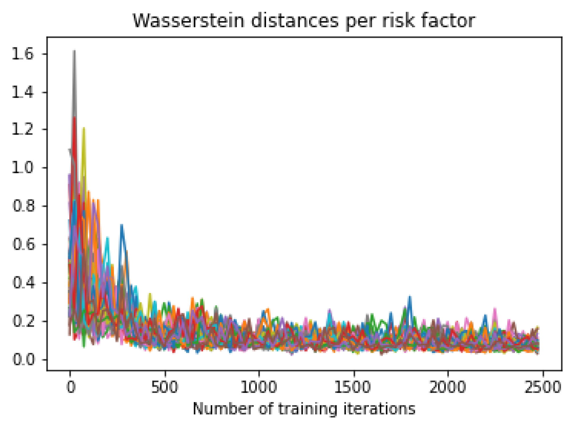
Appendix C. Optimization of GAN Architecture Using Wasserstein Distances

A full optimization is not possible as (see Motwani and Parmar (2020, Chapter 2)) the “selection of the GAN model for a particular application is a combinatorial exploding problem with a number of possible choices and their orderings. It is computationally impossible for researchers to explore the entire space.” Thus, in our study, we trained different GANs with the following:
  • The number of layers for generator and discriminator varying between 2, 4, 6 and 8;
  • The number of neurons for generator and discriminator varying between 100, 200 and 400.
During experiments, we fixed the following choices:
  • Batch size is M = 200
  • k = 10 training iterations for the generator in each discriminator training;
  • Dimension of the latent space is 200, and distribution of Z is multivariate normal with mean = 0 and std = 0.02;
  • Initialization of generator and discriminator using multivariate normal distribution with mean = 0 and std = 0.02.
  • We use LeakyReLu with α = 0.2 as activation functions except for the output layers, which use Sigmoid (for discriminator) and linear (for generator) activation functions. Additionally, we apply the regulation technique batch normalization after each of the hidden layers in the network.
  • We use the Adam optimizer with the parameters provided in Section 4.3 in Equation (2).
To arrive at one evaluation figure per GAN configuration, we aggregate 46 Wasserstein distances in each training iteration for each tested GAN configuration n by defining the following target function:
t f n = min t r a i n i n g i t e r a t i o n s max i = 1 , , 46 ( W i n ) , n = 1 , , 25
with W i n being the Wasserstein distance between the empirical distribution functions of the training and the generated data for risk factor i in GAN configuration n, as mentioned in Section 4.3. As in our case, we test 16 different configurations for the number of layers and nine different configurations for the number of neurons, and n varies between 1 and 25.
First, we run the GAN with 16 different configurations of layers for the discriminator D and the generator G with 200 neurons in each layer of the network. For each neural network, we used between two and eight layers in steps of two layers. The resulting t f n values are the following (the number of layer in D are in the columns, those of G in the rows).
Table A3. t f n -values for varying number of layers in both networks.
Number of Layers in D/G2468
20.1430.2520.6360.799
41.0360.1180.2350.435
60.9470.1720.1970.281
80.8070.1880.1710.178
The minimum of our target function t f n is reached for both neural networks possessing four layers (marked in bold). We cannot confirm in this experiment the thesis of Goodfellow (2016, p. 33) stating that the discriminator is usually deeper than the generator. What we can clearly see is that the number of layers plays an important role in the performance of the GAN.
We run the GAN with nine different configurations of neurons per hidden layer for discriminator D and generator G. In this experiment, we always set the number of neurons per layer as equal inside the respective neural network. The resulting t f n values are the following (the number of neurons per layer in D are in the columns, those of G in the rows).
Table A4. t f n values for varying number of neurons per layer in both networks.
Number of Neurons per Layer in D/G100200400
1000.1800.1170.125
2000.1850.1180.108
4000.1970.1160.124
The minimum of our target function t f n is reached for the discriminator posessing 400 and the generator possessing 200 neurons per layer (marked in bold). This is the configuration that we then used in our further research.

References

  1. Aggarwal, Alankrita, Mamta Mittal, and Gopi Battineni. 2021. Generative adversarial network: An overview of theory and applications. International Journal of Information Management Data Insights 1: 100004. [Google Scholar] [CrossRef]
  2. Albrecht, Peter, and Raimond Maurer. 2016. Investment-und Risikomanagement: Modelle, Methoden, Anwendungen. Stuttgart: Schäffer-Poeschel. [Google Scholar]
  3. Bennemann, Christoph. 2011. Handbuch Solvency II: Von der Standardformel zum internen Modell, vom Governance-System zu den MaRisk VA. Stuttgart: Schäffer-Poeschel. [Google Scholar]
  4. Borji, Ali. 2019. Pros and cons of gan evaluation measures. Computer Vision and Image Understanding 179: 41–65. [Google Scholar] [CrossRef] [Green Version]
  5. Chen, Yize, Pan Li, and Baosen Zhang. 2018. Bayesian renewables scenario generation via deep generative networks. Paper presented at the 2018 52nd Annual Conference on Information Sciences and Systems (CISS), Princeton, NJ, USA, March 21–23; pp. 1–6. [Google Scholar]
  6. Chollet, Francois. 2018. Deep Learning with Python. New York: Manning Publications. [Google Scholar]
  7. Cote, Marie-Pier, Brian Hartman, Olivier Mercier, Joshua Meyers, Jared Cummings, and Elijah Harmon. 2020. Synthesizing property & casualty ratemaking datasets using generative adversarial networks. arXiv arXiv:2008.06110. [Google Scholar]
  8. Danthine, Jean-Pierre. 2017. The interest rate unbound? Comparative Economic Studies 59: 129–48. [Google Scholar] [CrossRef]
  9. DAV (Deutsche Aktuarsvereinigung e.V.). 2015. Zwischenbericht zur Kalibrierung und Validierung spezieller ESG unter Solvency II. Ergebnisbericht des Ausschusses Investment der Deutschen Aktuarvereinigung e.V. Available online: https://aktuar.de/unsere-themen/fachgrundsaetze-oeffentlich/2015-11-09_DAV-Ergebnisbericht_Kalibrierung%20und%20Validierung%20spezieller%20ESG_Update.pdf (accessed on 26 April 2021).
  10. Denuit, Michel, Jan Dhaene, Marc Goovaerts, and Rob Kaas. 2006. Actuarial Theory for Dependent Risks: Measures, Orders and Models. Chichester: John Wiley & Sons. [Google Scholar]
  11. Deutsch, Hans-Peter. 2004. Derivate und Interne Modelle: Modernes Risikomanagement, 3rd ed. Stuttgart: Schäffer-Poeschel. [Google Scholar]
  12. Eckerli, Florian, and Joerg Osterrieder. 2021. Generative adversarial networks in finance: An overview. arXiv arXiv:2106.06364. [Google Scholar] [CrossRef]
  13. EIOPA. 2014. The Underlying Assumptions in the Standard Formula for the Solvency Capital Requirement Calculation. Available online: https://www.bafin.de/SharedDocs/Downloads/EN/Leitfaden/VA/dl_lf_solvency_annahmen_standardformel_scr_en.pdf (accessed on 26 April 2021).
  14. EIOPA. 2019. Technical Documentation of the Methodology to Derive Eiopas Risk-Free Interest Rate Term Structures. Available online: https://www.eiopa.europa.eu/sites/default/files/risk_free_interest_rate/12092019-technical_documentation.pdf (accessed on 26 April 2021).
  15. EIOPA. 2021a. YE2019 Comparative Study on Market & Credit Risk Modelling. Available online: https://www.eiopa.europa.eu/sites/default/files/publications/reports/2021-study-on-modelling-of-market-and-credit-risk-_mcrcs.pdf (accessed on 26 April 2021).
  16. EIOPA. 2021b. European Insurance Overview 2021. Available online: https://www.eiopa.europa.eu/sites/default/files/publications/reports/eiopa-21-591-european-insurance-overview-report.pdf (accessed on 26 April 2021).
  17. EIOPA MCRCS Project Group. 2020a. Specification of Financial Instruments and Benchmark Portfolios of the Year-End 2019 Edition of the Market and Credit Risk Modelling Comparative Study. Available online: https://www.eiopa.europa.eu/sites/default/files/toolsanddata/mcrcs_2019_instruments_and_bmp.xlsx (accessed on 26 April 2021).
  18. EIOPA MCRCS Project Group. 2020b. Market & Credit Risk Modelling Comparative Study (MCRCS), Year-End 2019 Edition: Instructions to Participating Undertakings for Filling out the Data Request. Available online: https://www.eiopa.europa.eu/sites/default/files/toolsanddata/mcrcs_year-end_2019_instructions_covidpostponed.pdf (accessed on 26 April 2021).
  19. European Commission. 2015. Commission delegated regulation (EU) 2015/35 of 10 October 2014 supplementing directive 2009/138/EC of the European parliament and of the council on the taking-up and pursuit of the business of insurance and reinsurance (Solvency II). Official Journal of European Union. Available online: https://eur-lex.europa.eu/legal-content/EN/TXT/PDF/?uri=CELEX:32015R0035&from=EN (accessed on 26 April 2021).
  20. Franco-Pedroso, Javier, Joaquin Gonzalez-Rodriguez, Jorge Cubero, Maria Planas, Rafael Cobo, and Fernando Pablos. 2019. Generating virtual scenarios of multivariate financial data for quantitative trading applications. The Journal of Financial Data Science 1: 55–77. [Google Scholar] [CrossRef]
  21. Fu, Rao, Jie Chen, Shutian Zeng, Yiping Zhuang, and Agus Sudjianto. 2019. Time series simulation by conditional generative adversarial net. arXiv arXiv:1904.11419. [Google Scholar] [CrossRef] [Green Version]
  22. Goodfellow, Ian. 2016. Nips 2016 tutorial: Generative adversarial networks. arXiv arXiv:1701.00160. [Google Scholar]
  23. Goodfellow, Ian, Jean Pouget-Abadie, Mehdi Mirza, Bing Xu, David Warde-Farley, Sherjil Ozair, Aaron Courville, and Yoshua Bengio. 2014. Generative adversarial networks. Communications of the ACM 63: 139–44. [Google Scholar] [CrossRef]
  24. Grasselli, Matheus R., and Alexander Lipton. 2019. On the normality of negative interest rates. Review of Keynesian Economics 7: 201–19. [Google Scholar] [CrossRef]
  25. Gründl, Helmut, Mirko Kraft, Thomas Post, Roman N Schulze, Sabine Pelzer, and Sebastian Schlütter. 2019. Solvency II-Eine Einführung: Grundlagen der neuen Versicherungsaufsicht, 2nd ed. Karlsruhe: VVW GmbH. [Google Scholar]
  26. Hallin, Marc, Gilles Mordant, and Johan Segers. 2021. Multivariate goodness-of-fit tests based on wasserstein distance. Electronic Journal of Statistics 15: 1328–71. [Google Scholar] [CrossRef]
  27. Henry-Labordere, Pierre. 2019. Generative Models for Financial Data. Available at SSRN 3408007. Available online: https://papers.ssrn.com/sol3/papers.cfm?abstract_id=3408007 (accessed on 26 April 2021).
  28. Ho, Yaoshiang, and Samuel Wookey. 2019. The real-world-weight cross-entropy loss function: Modeling the costs of mislabeling. IEEE Access 8: 4806–13. [Google Scholar] [CrossRef]
  29. Kokoska, Stephen, and Daniel Zwillinger. 2000. CRC Standard Probability and Statistics Tables and Formulae. Boca Raton: CRC Press. [Google Scholar]
  30. Kuo, Kevin. 2019. Generative synthesis of insurance datasets. arXiv arXiv:1912.02423. [Google Scholar]
  31. Lagerås, Andreas, and Mathias Lindholm. 2016. Issues with the smith–wilson method. Insurance: Mathematics and Economics 71: 93–102. [Google Scholar] [CrossRef] [Green Version]
  32. Lezmi, Edmond, Jules Roche, Thierry Roncalli, and Jiali Xu. 2020. Improving the robustness of trading strategy backtesting with boltzmann machines and generative adversarial networks. Available at SSRN 3645473. Available online: http://www.thierry-roncalli.com/download/rbm_gan_finance.pdf (accessed on 26 April 2021).
  33. Li, Ziqiang, Rentuo Tao, and Bin Li. 2020. Regularization and normalization for generative adversarial networks: A review. arXiv arXiv:2008.08930. [Google Scholar]
  34. Marti, Gautier. 2020. Corrgan: Sampling realistic financial correlation matrices using generative adversarial networks. Paper presented at the ICASSP 2020—2020 IEEE International Conference on Acoustics, Speech and Signal Processing (ICASSP), Barcelona, Spain, May 4–8; pp. 8459–63. [Google Scholar]
  35. Mazumdar, Eric, Lillian J. Ratliff, and S. Shankar Sastry. 2020. On gradient-based learning in continuous games. SIAM Journal on Mathematics of Data Science 2: 103–31. [Google Scholar] [CrossRef] [Green Version]
  36. Motwani, Tanya, and Manojkumar Parmar. 2020. A novel framework for selection of GANs for an application. arXiv arXiv:2002.08641. [Google Scholar]
  37. Ngwenduna, Kwanda Sydwell, and Rendani Mbuvha. 2021. Alleviating class imbalance in actuarial applications using generative adversarial networks. Risks 9: 49. [Google Scholar] [CrossRef]
  38. Ni, Hao, Lukasz Szpruch, Magnus Wiese, Shujian Liao, and Baoren Xiao. 2020. Conditional sig-wasserstein gans for time series generation. arXiv arXiv:2006.05421. [Google Scholar] [CrossRef]
  39. Pedersen, Hal, Mary Pat Campbell, Stephan L. Christiansen, Samuel H. Cox, Daniel Finn, Ken Griffin, Nigel Hooker, Matthew Lightwood, Stephen M. Sonlin, and Chris Suchar. 2016. Economic Scenario Generators: A Practical Guide. Available online: https://www.soa.org/globalassets/assets/Files/Research/Projects/research-2016-economic-scenario-generators.pdf (accessed on 26 April 2021).
  40. Pfeifer, Dietmar, and Olena Ragulina. 2018. Generating VaR scenarios under Solvency II with product beta distributions. Risks 6: 122. [Google Scholar] [CrossRef] [Green Version]
  41. S&P Ratings. 2018. Annual Global Corporate Default and Rating Transition Study. Available online: https://www.spratings.com/documents/20184/774196/2018AnnualGlobalCorporateDefaultAndRatingTransitionStudy.pdf (accessed on 26 April 2021).
  42. Salimans, Tim, Ian Goodfellow, Wojciech Zaremba, Vicki Cheung, Alec Radford, and Xi Chen. 2016. Improved techniques for training gans. arXiv arXiv:1606.03498. [Google Scholar]
  43. Smith, Andrew, and Tim Wilson. 2001. Fitting Yield Curves with Long Term Constraints. Technical Report. London: Bacon and Woodrow. [Google Scholar]
  44. Theis, Lucas, Aäron van den Oord, and Matthias Bethge. 2015. A note on the evaluation of generative models. arXiv arXiv:1511.01844. [Google Scholar]
  45. Viehmann, Thomas. 2019. Variants of the smith-wilson method with a view towards applications. arXiv arXiv:1906.06363. [Google Scholar]
  46. Wiese, Magnus, Lianjun Bai, Ben Wood, and Hans Buehler. 2019. Deep hedging: Learning to simulate equity option markets. arXiv arXiv:1911.017002019. [Google Scholar] [CrossRef] [Green Version]
  47. Wiese, Magnus, Robert Knobloch, Ralf Korn, and Peter Kretschmer. 2020. Quant gans: Deep generation of financial time series. Quantitative Finance 20: 1419–40. [Google Scholar] [CrossRef]
  48. Yoon, Jinsung, Daniel Jarrett, and Mihaela Van der Schaar. 2019. Time-series generative adversarial networks. In Advances in Neural Information Processing Systems. vol. 32, Available online: https://proceedings.neurips.cc/paper/2019/file/c9efe5f26cd17ba6216bbe2a7d26d490-Paper.pdf (accessed on 26 April 2021).
  49. Yu, Chong Ho. 2002. Resampling methods: Concepts, applications, and justification. Practical Assessment, Research, and Evaluation 8: 19. [Google Scholar]
Figure 1. Composition of the MCRCS asset-only benchmark portfolios BMP1–BMP10.
Risks 10 00199 g001
Figure 2. Architecture of GANs training procedure according to Chen et al. (2018, p. 2).
Risks 10 00199 g002
Figure 3. Scatterplots of results of a GAN for a two-dimensional data distribution at different training iterations: red = empirical data; blue = generated data.
Risks 10 00199 g003
Figure 4. Scatterplots of four different risk factor pairs: empirical vs. generated data by a GAN.
Risks 10 00199 g004
Figure 5. Histogram of minimum distances of the generated data points to the empirical data points.
Risks 10 00199 g005
Figure 6. Workflow of a GAN-based internal model.
Risks 10 00199 g006
Figure 7. Comparison of the simulated shifts for the corporate and sovereign credit spread risk factors; representation based on our own results (blue dots) and EIOPA (2021a, pp. 25–26) (gray boxes).
Risks 10 00199 g007
Figure 8. Comparison of the simulated shifts for equity risk factors, and representation based on own results (blue dots) and EIOPA (2021a, p. 27) (gray boxes).
Risks 10 00199 g008
Figure 9. Comparison of the simulated shifts (left: up, right: down) for interest rate risk factors; representation based on own results (blue dots) and EIOPA (2021a, p. 22) (gray boxes).
Risks 10 00199 g009
Figure 10. Comparison of the asset-only benchmark portfolios; representation based on own results (blue dot) and EIOPA (2021a, p. 16) (gray boxes).
Risks 10 00199 g010
Figure 11. Comparison of the liabilities-only benchmark portfolios; representation based on own results (blue dot) and EIOPA (2021a, p. 25) (gray boxes).
Risks 10 00199 g011
Figure 12. Comparison of the combined asset-liability benchmark portfolios; representation based on own results (blue dot) and EIOPA (2021a, p. 14) (gray boxes).
Risks 10 00199 g012
Figure 13. Comparison of the implied percentiles for the backtesting exercise; representation based on own results (blue dots) and EIOPA (2021a, pp. 19–20) (gray boxes).
Risks 10 00199 g013
Figure 14. Comparison of the joint quantile exceedance for selected risk factors; representation based on own results (blue dots) and EIOPA (2021a, p. 35) (gray boxes).
Risks 10 00199 g014
Figure 15. Comparison of the GAN risk charges in 20 different runs versus MCRCS study for four risk factors.
Risks 10 00199 g015
Figure 16. Development of the Wasserstein distances for all 46 risk factors during GAN training iterations.
Risks 10 00199 g016
Table 1. Worst case losses of all benchmark portfolios and implied percentiles of the GAN-based model.
Benchmark PortfolioWorstCase(P) α P , GAN
BMP1−2.8%13.5%
BMP2−2.5%19.2%
BMP3−2.8%15.6%
BMP4−2.7%19.6%
BMP5−2.4%13.3%
BMP6−2.8%10.9%
BMP7−7.8%2.3%
BMP8−2.7%16.2%
BMP9−3.7%21.6%
BMP10−6.1%5.9%
L1−15.2%5.4%
L2−4.3%15.8%
BMP1+L1−58.2%3.5%
BMP3+L1−64.5%0.9%
BMP7+L1−67.1%6.8%
BMP9+L1−41.3%7.1%
BMP10+L1−89.9%3.4%
BMP1+L2−30.9%3.8%
BMP3+L2−34.8%2.5%
BMP7+L2−53.4%3.9%
BMP9+L2−26.8%13.6%
BMP10+L2−65.6%3.6%
Publisher’s Note: MDPI stays neutral with regard to jurisdictional claims in published maps and institutional affiliations.

