Assessing the Market Risk on the Government Debt of Kazakhstan and Bulgaria in Conditions of Turbulence

Abstract

The purpose of this publication is to quantify and compare the market risk on the external government debt of Kazakhstan and Bulgaria in the conditions of COVID-19, the emerging energy crisis, and the coup attempt in the first country. In particular, the authors invest the market risk of sovereign bonds issued on global financial markets. Market risk is assessed both as a single issue and at a portfolio level using the Value-at-risk approach. Sixteen samples with historical observations of all issues of Kazakhstan’s and Bulgarian Sovereign Bonds issued on the international financial markets were formed. The duration method was used in the calculation of Delta normal bond VaR and CVaR. It was found that with the same credit rating, similar portfolio duration levels, similar GDP per capita, Debt (% of GDP), and Debt Per Capita, the market risk on their portfolio differed significantly. The comparison of risk levels between the two portfolios was made by six indicators–two indicators measuring linearly the sensitivity of bond prices to changes in market interest rates (Weighted average Macaulay duration and Weighted average modified duration) and four downside indicators (Undiversified VaR, Diversified VaR, Undiversified CVaR, amd Diversified CVaR). The return/risk performance of both portfolios was assessed by the Sharpe ratio in three variants (SR Undiversified VaR, SR Diversified VaR, and SR Diversified CVaR). When evaluating the bond portfolio VaR and CVaR, a practical version of the Duration method was proposed, which allows the use of an unlimited number of assets, taking into account the correlations between yield returns and historical price volatility.

1. Introduction

In the last few years, the number of published studies related to the impact of COVID-19 on various market segments of the market economy has increased (Bouri et al. 2021; Naseem et al. 2021; Sun et al. 2021). Azam, M. Q., Hashmi, N. I., Hawaldar, I. T., Alam, M. S. and Baig, M. A. analyzes to investigate the overconfidence bias in 12 cyclical and defensive sectors in pre-and during COVID-19 periods using daily data (Azam et al. 2022). They use vector autoregression (VAR) along with impulse response functions (IRFs) The final results show that in the pre COVID-19 phase overconfidence bias is more prevalent in all the cyclical sectors.

On the other hand, over the last decade, financial markets have attached great importance to ethical and socially responsible values (Lee and Suh 2022; Giaretta and Chesini 2021). Socially responsible companies whose values are aligned with the United Nations Sustainable Development Goals (UN SDGs) contribute to creating wealth and long-term economic and social value (Lassala et al. 2021).

Measuring market risk in fixed-term financial instruments continues to pose challenges to scholars and practitioners in modern financial risk management. When assessing the risk of interest-bearing bonds, it is not always possible to calculate market risk using the three approaches recommended by the Basel Committee on Banking Supervision or, if possible, the calculation process is complex and time-consuming (Sousa et al. 2019). The calculation algorithms of VaR applied here are relatively more complex and have several specifics compared to the calculation of market risk for stocks, exchange rates, commodities, or interest rates. The accuracy of the forecast calculations in the calculation of VaR for interest-bearing bonds is a guarantee of a significantly higher number of assumptions than the assets referred to above.

The reasons for this paper are related to two research objectives. The first is the assessment and comparison of market risk on the external government debt of Kazakhstan and Bulgaria in the conditions of COVID-19, the emerging energy crisis, as well as the attempted coup in the first country. The second is the need to present the algorithm and results of a practical method that allows the use of an unlimited number of fixed-term financial assets, taking into account the correlations between yield returns and the volatility of historical prices. In the evaluation of bond VaR, a variant of the Duration method was used, in which there is no limit on the number of fixed income instruments, and the correlations between yield returns are taken into account. Two portfolios of eight bonds each of the two countries’ foreign debt have been drawn up.

Current work is limited to market risk on the external debt of Kazakhstan and Bulgaria, as credit risk remains out of the focus of the study. The object of study is external debt in the form of sovereign bonds issued on global financial markets. The sample frame of the study is limited to a little over two years (from 1 January 2020 to 8 January 2022). The purpose of this time constraint is to cover the price volatility of the COVID-19 pandemic, the coup attempt in Kazakhstan, and the beginning of the emerging energy crisis.

On the other hand, the financial market provides a mechanism for aggregating information of heterogeneous traders, who have different beliefs, knowledge and trading strategies and interactions between heterogeneous traders and their impacts on price quotations are proven (Gong et al. 2021).

The Value-at-risk approach has established itself over the last few decades as the dominant method of management and monitoring market risk in the risk management industry. Moreover, it is already regulated as an international regulatory standard in banking practice through the regulatory frameworks created by Basel Accords and Basel II in 2006 (Basel 2006), Basel III in 2016 (Basel 2016) and its amendment in 2019 (Minimum capital requirements for Market Risk, Basel 2019). These promoted VaR as a part of sound risk analysis methods.

The term Value-at-risk is believed to have been used for the first time in 1993’s Derivatives: Practices and Principles report of the Group of Thirty (G30) (Holton 2002). In theory and practice, only its abbreviation VaR is more often used instead of the full name. VaR gained widespread popularity through JP Morgan’s 1994 Risk Metrics Technical Document (Morgan 1994).

Value-at-risk is a statistical measure of market risk. It represents a summary quantitative assessment of the risk exposure for a single asset or investment portfolio. Its main advantage is the quantification of market risk in a single value. Value-at-risk shows what the expected maximum loss that an investor would incur for a certain period under a certain level of probability, under normal market conditions. This indicator belongs to the group of downside risk measures and summarizes in one figure all the market risks that an investor has taken on the various transactions. Downside risk measures do not weigh equally the deviations from the average return on an asset. They measure the degree of variability (risk) based on negative values for profitability or those below a certain target value, which cause losses to the financial institution. The Basel Committee on Banking Supervision recommends three main approaches when using the VaR methodology for market risk assessment—Delta normal (parametric VaR), Historical simulation, and Monte Carlo simulation. The latest addition to Basel III from 2019 recommends using Conditional value at risk (CVaR) (Minimum capital requirements for Market Risk, Basel 2019).

Each of the listed methods is used in different varieties and modifications, depending on the views and assumptions of the respective risk manager and the methods used in forecasting volatility. It should be borne in mind that the value of VaR is very sensitive to the calculation method used and the assumptions made in the model framework. In this regard, especially after the financial crisis of 2007, critics of the VaR approach became more active. VaR was the subject of a public debate between Philippe Jorion (Jorion 2007) and Nassim Taleb (Taleb 1997) Taleb has established himself as one of the zealous critics of the VaR methodology. In the scientific dispute with Prof. Philippe Jorion he argued “suspend the current version of VAR as potentially dangerous malpractice while his is to supplement it with other methods”, I conjecture that the methods we currently use to measure such tail probabilities are flawed. Andreas Krause (Krause 2003) shows that VaR is not always a good risk measure and is often prone to substantial measurement error. The author concludes that VaR remains a useful risk management tool when appropriately applied with an understanding of its limitations.

Large banks and corporations are committing significant resources and the most prominent members of the academic community to create models that provide them with a competitive advantage in terms of minimizing investment losses by more accurately measuring and forecasting market risk (Harle et al. 2016).

The calculation procedure of VaR for bonds differs significantly from that used for capital assets such as stocks, commodities, precious metals, and currencies. Bond VaR, unlike targeted capital assets, cannot be directly calculated using historical prices, because “bonds historical returns are not stationary, as they tend to zero as time matures approaches the so-called pull-to-pare effect. Returns convergence to zero result from bond prices convergence to their par value at maturity” (Sousa et al. 2019). In addition to the pull-to-pare effect in the calculation of bond VaR, additional factors must be taken into account as the yield-price relationship, daily change in maturities, and the timing of future cash flows. It should also be borne in mind that different maturities are associated with different risks, the relationship is approximately functional only with the same credit rating. Despite these reasons, some researchers directly use historical prices in a similar way as in stock’s VaR when calculating bond VaR (Obadovic et al. 2016; Samanta et al. 2010; Vlaar 2000).

In modern risk management theory, three main methods have been identified in the calculation of bond VaR within the modeling frameworks approved by the Basel Committee on Banking Supervision. The targeted methods apply different modeling procedures, accept different approximations and assumptions in the model frameworks. These three methods are known as:

• Portfolio mapping method;
• Duration method;
• Pull Price method.

The idea of portfolio mapping is considered to have been proposed for the first time and developed by the research department of the American investment bank JPMorgan. Portfolio mapping refers to the process of aggregating the risk factors and replacing each bond with its risk exposure. Methods of Mapping Portfolios of Fixed Income Securities are (Jorion 2007):

• Principal mapping;
• Cash Flow Mapping;
• Duration mapping.

The principal bond mapping only considers the timing of the redemption of the bond’s face value. For this reason, it is quite an inaccurate way to calculate VaR. The duration mapping method is very similar to principal mapping and here the leading criterion for mapping is the portfolio duration. First, the current values of the expected cash flows are calculated, then the portfolio duration is found and finally the diversified portfolio VaR is found by interpolating return VaRs for a zero-coupon bond with relevant maturities to portfolio duration. The duration mapping method is considered more accurate than the principal bond mapping but is inferior to the Pull Price method and Duration method.

The Cash Flow Mapping first allocates in a time all the resent values of cash flows in the bond portfolio including principal or coupon payments and treats them such as zero-coupon bonds with standard maturities (Jorion 2007; Mina and Xiao 2001). Undiversified VaR is then calculated as the sum of the products of the present values of the cash flows and the return VaRs of the zero-coupon bonds. Diversified VaR is obtained by the calculation algorithm of the portfolio standard deviation as a product of the correlation matrix of zero-coupon bonds and the vector of individual undiversified VaRs.

The Pull Price method is relatively new compared to the others. It was discovered by a team of researchers from the University of Lisbon School of Economics & Management (Sousa 2012). The main idea of this method is to calculate VaR through historical simulation using historical prices similar to the original calculation algorithm. According to the majority of researchers in this field, historical returns cannot be used directly to compute VaR by historical simulation because the maturities of interest rates implied by historical prices are not the relevant maturities at which VaR is computed. To overcome this problem, Portuguese researchers replaced the original historical returns with adjusted bonds historical returns that could be used directly in the VaR computation (Sousa et al. 2014). Later, they refined and developed their idea (Sousa et al. 2019).

The Duration method calculates VaR using Duration or Convexity, which measures a bond’s price sensitivity to changes in market interest rates. Macaulay’s duration and respectively modified duration represent a simplified linear dependence of the price-interest rate relationship and are a suitable model for small interest rate changes. The model that Convexity includes has a nonlinear character and is closer to reality. Some authors suggest using exponential duration as a more accurate estimation of interest rate risk (Livingston and Zhou 2005; Di Asih and Abdurakhman 2021).

Next, the Duration method VaR is the change in price corresponding to the worst, relevant quantile, change in yield. The calculation algorithm and modeling procedure of the Duration method will be presented in detail in part four.

Bond market risk is composed of two types of risk—risk arising from interest rate volatility and risk arising from market price volatility to a lesser extent. Most models for assessing and forecasting market risk in interest-bearing bonds focus mainly on yield volatility, ignoring price volatility as a separate risk factor. Three factors that influence a bond’s market price are the market interest rates, the time to maturity but the issuer also, and some other reasons to a small extent.

2. Results

In this study, we evaluate the market risk on the government debt of Kazakhstan and Bulgaria by calculating the sovereign bond value at risk. All presented indicators of VaR and CVaR were calculated with a confidence level of 99%. The samples include historical daily data and cover the period from 1 January 2020 to 8 January 2022 (from the beginning of the COVID-19 pandemic to the end of the coup attempt in Kazakhstan). From which, 16 samples were formed, each of which includes 512 observations except for issues with a later date from 1 January 2020.

2.1. Market Risk Indicators of Kazakhstan’s Sovereign Bonds

Table 1. The Value at risk for Kazakhstan’s Sovereign Bonds.

ISIN:	Code	Day	10 Days	Year
XS1907130246	Kz18/23	−2.410%	−7.621%	−38.104%
XS1120709669	Kz14/24	−0.302%	−0.954%	−4.768%
XS1263054519	Kz15/25	−0.351%	−1.109%	−5.545%
XS2050933899	Kz19/26	−0.835%	−2.641%	−13.205%
XS1901718335	Kz18/28	−1.015%	−3.208%	−16.041%
XS2050933626	Kz19/34	−0.770%	−2.435%	−12.174%
XS1120709826	Kz14/44	−0.792%	−2.504%	−12.519%
XS1263139856	Kz15/45	−1.270%	−4.015%	−20.076%
	Undiversified VaR	−7.743%	−24.49%	−122.43%

Source: Calculated by the authors; ISIN: International Securities Identification Number.

displays the calculated individual VaRs for each bond along with the undiversified VaR of Kazakhstan’s Sovereign Bonds portfolio. The highest values are observed for the issue with the shortest maturity (Kz18/23) and the one with the longest maturity (Kz15/45).

The maximum loss calculated with a probability of 99% for Kz18/23 emissions is expected to be up to −2.410% on a one-day basis, up to −7.621% for 10 days and up to −8.104%, respectively, for a year. Bond Kz15/45 has values of one-day VaR = −1.270%, respectively, VaR = −4.015% for 10 days% and VaR = −20.076% for the year.

It could be seen in Figure 1. that the coup attempt in Kazakhstan did not significantly affect the volatility of the yield return and YTM of riskiest bond issue Kz18/23. The highest levels of negative values of yield return were registered on 20 March 2020 in the amount of −0.57%, on 8 June 2021 in the amount of −1.25% decrease, on 17 September 2021 in the amount of −0.77% on daily basis.

Table 2. The Conditional Value at risk for Kazakhstan’s Sovereign Bonds.

CVaR	Day	10 Days	Year
Kz18/23	−2.761%	−8.731%	−43.654%
Kz14/24	−0.345%	−1.092%	−5.462%
Kz15/25	−0.402%	−1.271%	−6.353%
Kz19/26	−0.957%	−3.026%	−15.128%
Kz18/28	−1.162%	−3.676%	−18.378%
Kz19/34	−0.882%	−2.789%	−13.947%
Kz14/44	−0.907%	−2.868%	−14.342%
Kz15/45	−1.455%	−4.600%	−23.001%
Undiversified CVaR	−8.871%	−28.05%	−140.27%

Source: Calculated by the authors.

displays the calculated individual CVaRs for each bond along with the undiversified CVaR of Kazakhstan’s Sovereign Bonds portfolio. The conditional value at risk, also known as the expected shortfall or the conditional tail expectation a more sensitive risk measure in the tail of the distribution.

The highest CVaR values are observed for the emission with the shortest maturity (Kz18/23) and the emission with the longest maturity (Kz15/45). These results can be interpreted as follows. If the maximum loss calculated with a probability of 99% for Kz18/23 emission exceeds the calculated VaR values (in Table 1) then its values are expected to be: CVaR = −2.761% for a one-day period, respectively, CVaR = −8.731% for 10 days and CVaR = −43.654% for the year. The other issue where high levels of conditional value at risk are observed is Kz15/45. If the maximum loss exceeds the calculated values of VaR (in Table 1) then the expected value of the loss for one day will be −1.455%, respectively, −4.6% for 10 days and −23% for the year.

It could be seen in Figure 2 that the coup attempt in Kazakhstan did not have a significant impact on the volatility of the yield return and YTM of bond issue Kz15/45. The highest levels of negative values of yield return were registered on 27 March 2020 in the amount of −0.853%.

The observed values of the correlations between the YTM returns are quite low and even a negative dependence is observed, which is atypical when using the historical yield curve (

Table 3. YTM return correlation matrix of Kazakhstan’s Sovereign Bonds.

	Kz18/23	Kz14/24	Kz15/25	Kz19/26	Kz18/28	Kz19/34	Kz14/44	Kz15/45
Kz18/23	1.0000	0.0028	0.0352	0.0222	0.0287	−0.0172	0.0391	0.0660
Kz14/24	0.0028	1.0000	0.3589	0.3468	0.2401	0.2147	0.3455	0.2969
Kz15/25	0.0352	0.3589	1.0000	0.3322	0.2389	0.3806	0.3415	0.4870
Kz19/26	0.0222	0.3468	0.3322	1.0000	0.6186	0.4137	0.5428	0.3968
Kz18/28	0.0287	0.2401	0.2389	0.6186	1.0000	0.3577	0.4411	0.3384
Kz19/34	−0.0172	0.2147	0.3806	0.4137	0.3577	1.0000	0.2990	0.5144
Kz14/44	0.0391	0.3455	0.3415	0.5428	0.4411	0.2990	1.0000	0.5264
Kz15/45	0.0660	0.2969	0.4870	0.3968	0.3384	0.5144	0.5264	1.0000

Source: Calculated by the authors.

).

Calculated values Diversified VaR = 4.599% and Diversified CVaR = 5.269% allow us to draw the following conclusions. It could be concluded 99% certain that this bond portfolio will not lose more than 4.599% over the next day or if the loss still exceeds this value its expected amount will be around 5.269% assuming ordinary market conditions.

2.2. Market Risk Indicators of Bulgarian’s Sovereign Bonds

Table 4. The Value at risk for Bulgarian’s Sovereign Bonds.

Bonds	Day	10 Days	Year
BG15/22	−0.050%	−0.157%	−0.785%
BG16/23	−0.770%	−2.436%	−12.182%
BG14/24	−0.121%	−0.382%	−1.909%
BG15/27	−4.587%	−14.505%	−72.524%
BG16/28	−1.075%	−3.401%	−17.003%
BG20/30	−0.432%	−1.365%	−6.827%
BG15/35	−0.834%	−2.637%	−13.183%
BG20/50	−0.574%	−1.816%	−9.079%
Undiversified VaR	−8.443%	−26.698%	−133.492%

Source: Calculated by the authors.

displays the calculated individual VaRs for each bond along with undiversified VaRs of the Bulgarian’s Sovereign Bonds portfolio. The highest values are observed for bond BG15/27.

The maximum loss calculated with a probability of 99% for emission BG15/27 is expected to be up to −4.587% on a daily basis, respectively, to −14.505% for 10 days and up to −17.003% for a year. The maximum loss calculated by Undiversified VaR with a probability of 99% for the entire portfolio is expected to be −8.443% for one day, and up to −26.698% for a period of 10 days.

It could be seen in Figure 3 that the highest levels of negative values of yield return are registered in those periods when YTM also becomes negative. Here in bond issue BG15/27, unlike the riskiest Kazakhstan’s Sovereign Bonds, we observe periods of negative YTM values. The highest levels of negative values of yield return were registered on 13 November 2020 in the amount of −0.45%, on 25 January 2021 in the amount of −0.356%, and 23 July 2021 in the amount of −0.294% daily.

Table 5. The Conditional Value at risk for Bulgarian’s Sovereign Bonds.

Bonds	Day	10 Days	Year
BG15/22	−0.057%	−0.180%	−0.899%
BG16/23	−0.883%	−2.791%	−13.956%
BG14/24	−0.138%	−0.437%	−2.187%
BG15/27	−5.255%	−16.618%	−83.089%
BG16/28	−1.232%	−3.896%	−19.480%
BG20/30	−0.495%	−1.564%	−7.821%
BG15/35	−0.955%	−3.021%	−15.104%
BG20/50	−0.658%	−2.080%	−10.401%
Undiversified CVaR	−9.673%	−30.587%	−152.937%

Source: Calculated by the authors.

displays the calculated individual CVaRs for each bond along with the undiversified CVaR of the Bulgarian’s Sovereign Bonds portfolio. The highest CVaR values are observed for issues BG 15/27 and BG 16/28. These results can be interpreted as follows. If the maximum loss calculated with a probability of 99% for BG 15/27 issues exceeds the calculated VaR values (Table 4) then its values are expected to be around: CVaR = −5.255% for a day period, respectively, CVaR = −16.618% for 10 days and CVaR = −83.089% for the year. The other issue where high levels of conditional value at risk are observed was BG 16/28. If the maximum loss exceeds the calculated values of VaR (Table 4) then the expected value of the loss for one day will be around −1.232%, respectively, −3.896% for 10 days and −19.480% for a year.

The observed values of the correlations between the YTM returns are quite low and even a negative dependence is observed, which is atypical when using the historical yield curve (

Table 6. YTM return correlation matrix of Bulgarian’s Sovereign Bonds.

	BG15/22	BG16/23	BG14/24	BG15/27	BG16/28	BG20/30	BG15/35	BG20/50
BG15/22	1.0000	0.0072	0.1712	0.0059	−0.0485	−0.0074	0.0587	0.0035
BG16/23	0.0072	1.0000	−0.0781	0.0107	−0.1644	−0.0953	−0.2099	−0.1993
BG14/24	0.1712	−0.0781	1.0000	0.0044	−0.0032	−0.0534	−0.0196	−0.0382
BG15/27	0.0059	0.0107	0.0044	1.0000	−0.0258	0.0243	0.1076	0.1440
BG16/28	−0.0485	−0.1644	−0.0032	−0.0258	1.0000	0.1961	0.1764	0.2522
BG20/30	−0.0074	−0.0953	−0.0534	0.0243	0.1961	1.0000	0.4143	0.3785
BG15/35	0.0587	−0.2099	−0.0196	0.1076	0.1764	0.4143	1.0000	0.5444
BG20/50	0.0035	−0.1993	−0.0382	0.1440	0.2522	0.3785	0.5444	1.0000

Source: Calculated by the authors.

).

The calculated values Diversified VaR = −5.151% and Diversified CVaR = −5.901% allow us to draw the following conclusions. It could be concluded 99% certain that this bond portfolio will not lose more than −5.151% over the next day or if the loss still exceeds this value its expected size will around −5.901% assuming the normal market conditions.

Table 7. Risk measures of Kazakhstan and Bulgarian bond portfolios.

Risk Measures	Kazakhstan Bond Portfolio	Bulgaria Bond Portfolio
Undiversified VaR	−7.743%	−8.443%
Diversified VaR	−4.599%	−5.151%
Undiversified CVaR	−8.871%	−9.673%
Diversified CVaR	−5.269%	−5.901%
SR diversified VaR	0.8950	0.4085

Source: Calculated by the authors.

shows the calculated values of the indicators for measuring the market risk of the bond portfolio of Kazakhstan and Bulgaria on daily basis. It can be seen that in all risk measures Bulgarian government bond portfolio is riskier than Kazakhstan. The expected loss, if it occurs on a daily basis is −8.87% for Kazakhstan against −9.67% for Bulgaria in the undiversified portfolio.

Sharpe ratio is used in the last row of Table 7 to evaluate both portfolios in terms of their Reward-to-risk effectiveness. The Sharpe ratio is a commonly used risk-adjusted measure of portfolio performance.

3. Discussion

The purpose of this manuscript was to assess and compare the market risk on the external debt of Bulgaria and Kazakhstan in the COVID-19 pandemic, the developing energy crisis, and the attempted coup in Kazakhstan that took place between 04.01–7.01.22. Kazakhstan and Bulgaria are two countries, although spatially distant, which show quite similar debt indicators in relative terms in recent years. Kazakhstan and Bulgaria are chosen because these are two countries, although spatially distant, which show quite similar debt indicators in relative terms in recent years.

Table 8. Macroeconomic indicators for the national economies of Bulgaria and Kazakhstan.

2020	Bulgaria	Kazakhstan
Annual GDP	$69,209M	$171,240M
GDP per capita	$10,006	$9131
Debt ($M)	17,347	45,194
Debt (%GDP)	24.70%	26.33%
Debt Per Capita	$2508	$2410
Deficit ($M)	−2791	−12,066
Deficit (%GDP)	−4.00%	−7.03%
Expenditure ($M)	29,281.6	42,088.4
Expenditure (%GDP)	41.80%	24.52%
Expenditure Per Capita	$4234	$2244
Moody’s Rating	Baa1	Baa2
Fitch Rating	BBB	BBB
Corruption Index	44	38

Source: https://countryeconomy.com (accessed on 1 March 2022).

presents up-to-date information on the most important macroeconomic indicators for the national economies of Bulgaria and Kazakhstan.

Table 8 shows that the two countries have the same credit rating, similar GDP per capita, Debt (% of GDP), and Debt Per Capita.

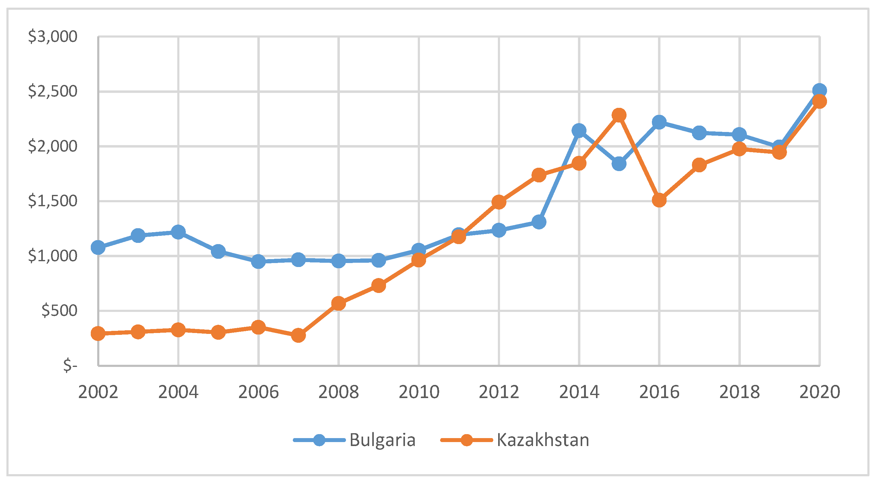
Figure 4 shows the dynamics of the Government debt per capita (USD) indicator in Kazakhstan vs. Bulgaria. It can be seen that over the last decade there has been convergence in terms of Government debt per capita, and in the last few years, the values have been almost identical.

Figure 5 illustrates the dynamics in the development of the Government debt (percentage of GDP) indicator in Bulgaria and Kazakhstan. Here we also see a similar variation of the indicator for the last decade and almost identical values in the two countries for the last three years.

Although in the last decade the two countries have seen almost identical coincidences in the movement of the Long Term Rating, both in terms of Foreign and Local currency, the Key Rating Drivers are different. The Positive Outlook on Bulgaria’s Long-Term Foreign and Local-Currency Issuer Default Ratings are linked to the prospect of euro adoption, which would lead to significant improvements in external metrics, prospects of substantial EU funding for investment, and a broad commitment to macro and fiscal stability (Fitch Credit Rating Agency 2022).

On the other hand, the positive outlook on Kazakhstan’s rating is related to the strong fiscal and external balance sheets, which have shown resilience during the coronavirus pandemic. Analysts note that the country’s public debt has remained at a low level, while net sovereign assets are much higher. Moreover, according to Fitch’s forecast, Kazakhstan will remain a net creditor in the medium term (Kazkhstan 2022).

Table 9. Fitch’s sovereign ratings for Bulgaria and Kazakhstan.

Kazakhstan				Bulgaria
Date	Long Term Rating		Short Term Rating	Date	Long Term Rating		Short Term Rating
	Foreign Currency	Local Currency	Foreign Currency		Foreign Currency	Local Currency	Foreign Currency
21.2.2020	BBB	BBB	F2	21.2.2020	BBB	BBB	F2
6.9.2019	BBB	BBB	F2	23.8.2019	BBB	BBB	F2
22.3.2019	BBB	BBB	F2	22.3.2019	BBB	BBB	F2
28.9.2018	BBB	BBB	F2	16.11.2018	BBB	BBB	F2
13.4.2018	BBB (Stable)	BBB	F2	1.6.2018	BBB (Stable)	BBB	F2
20.10.2017	BBB (Stable)	BBB	F2	1.12.2017	BBB (Stable)	BBB	F2
21.4.2017	BBB (Stable)	BBB	F2	2.6.2017	BBB− (Positive)	BBB-	F3
28.10.2016	BBB(Stable)	BBB	F2	2.12.2016	BBB− (Stable)	BBB-	F3
22.7.2016	BBB (Stable)	BBB	F2	22.7.2016	BBB− (Stable)	BBB-	F3
29.4.2016	BBB (Stable)	BBB	F2	3.6.2016	BBB− (Stable)	BBB	F3
30.10.2015	BBB+ (Stable)	A-	F2	4.12.2015	BBB− (Stable)	BBB	F3
1.5.2015	BBB+	A-	F2	19.6.2015	BBB−	BBB	F3
7.11.2014	BBB+ (Stable)	A-	F2	19.12.2014	BBB−	BBB	F3
8.10.2014	BBB+ (Stable)	A-	F2	4.7.2014	BBB− (Stable)	BBB	F3
9.5.2014	BBB+ (Stable)	A-	F2	27.6.2014	BBB− (Stable)	BBB	F3
14.11.2013	BBB+ (Stable)	A-	F2	12.7.2013	BBB− (Stable)	BBB	F3
20.11.2012	BBB+ (Stable)	A-	F2	17.7.2012	BBB− (Stable)	BBB	F3
21.11.2011	BBB	BBB+	F3	13.12.2011	BBB− (Stable)	BBB	F3

Source: www.fitchratings.com/research/sovereigns/bulgaria-17-02-2022 (accessed on 1 February 2022).

shows the comparison of credit ratings in Kazakhstan and Bulgaria over the last decade.

Table 10. Return/risk performance indicators for the bond portfolio of Bulgaria and Kazakhstan (daily basis).

Return/Risk Measures	Kazachstan Bond Portfolio	Bulgaria Bond Portfolio	Difference
Undiversified VaR	−7.74%	−8.44%	0.70%
Diversified VaR	−4.60%	−5.15%	0.55%
Undiversified CVaR	−8.87%	−9.67%	0.80%
Diversified CVaR	−5.27%	−5.90%	0.63%
Return of portfolio	4.12%	2.10%	2.01%
Weighted average Macaulay duration	7.113	7.144	0.031
Weighted average modified duration	5.171	5.571	0.400
SR (Undiversified VaR)	0.5316	0.2492	0.282
SR (Diversified VaR)	0.8950	0.4085	0.487
SR (Diversified CVaR)	0.7812	0.3565	0.425

Source: Calculated by the authors.

presents the calculated values of selected indicators for the assessment of return/risk performance for the bond portfolio of Bulgaria and Kazakhstan on daily basis. The comparison of risk levels between the two portfolios was made by six indicators—two indicators measuring linearly the sensitivity of bond prices to changes in market interest rates (Weighted average Macaulay duration and Weighted average modified duration) and four downside indicators Undiversified VaR, Diversified VaR, Undiversified CVaR, and Diversified CVaR). The return/risk performance of both portfolios was assessed by Sharpe ratio in three variants (SR (Undiversified VaR), SR (Diversified VaR), and SR (Diversified CVaR).

Regarding the sensitivity of portfolio bond prices to changes in market interest rates, the Weighted average Macaulay indicator duration almost shows no difference between the two portfolios (0.031 years ≈ 12 days), the difference calculated by the Weighted average modified duration is 0.4 years (5 months in favor of Kazakhstan bond portfolio).

The VaR and CVaR values (calculated as Undiversified or Diversified) of the two debt portfolios show differences ranging between 0.55% and 0.8%. This difference is significant because it is calculated daily. It is obvious that despite the extreme events of the coup attempt from the beginning of January 2022, Kazakhstan’s sovereign bond portfolio is much less risky than Bulgaria’s, although the latter is in Europe and is a member of the EU and NATO for more than 15 years1.

The portfolio daily difference in Undiversified value at risk (VaR) is 0.7%, in Undiversified conditional value at risk CVaR is 0.8%, Diversified VaR 0.55%, and Diversified CVaR 0.63% in favor of Kazakhstan bond portfolio.

The Sharpe ratio is best used to evaluate portfolios with similar risk characteristics over the same period. The calculated Sharpe ratio values through SR (Diversified VaR), SR (Diversified CVaR) for both portfolios show from the point of view of large investors that Kazakhstan’s bond portfolio is more than twice (2.19) more efficient than Bulgaria’s bond portfolio.

4. Materials and Methods

The market risk research on the government debt of the two countries was limited to the external debt traded on the international financial markets, current as of 8 January 2022 excluding bank loans denominated in different currencies. All data used in the present study are publicly available. Data on macroeconomic indicators are publicly available at: https://countryeconomy.com, and market quotations used in calculating market risk indicators are publicly available on the Frankfurt Stock Exchange website www.boerse-frankfurt.de.

Kazakhstan’s foreign sovereign debt is up to date as of 8 January 2022, which is traded on international stock exchanges, is structured by eight treasury interest-bearing bonds. Their main parameters are given in

Table 11. Kazakhstan’s Sovereign Bonds parameters.

ISIN:	Coupon	Interest Payment Count	Minimum Tradeable Unit	Issue Date	Issue Volume	Issue Currency	Maturity
XS1907130246	1.550%	yearly	100,000	11/9/2018	525,000,000	EUR	11/9/2023
XS1120709669	3.875%	semiannual	200,000	10/14/2014	1,500,000,000	USD	10/14/2024
XS1263054519	5.125%	semiannual	200,000	7/21/2015	2,500,000,000	USD	7/21/2025
XS2050933899	0.600%	yearly	100,000	9/30/2019	500,000,000	EUR	9/30/2026
XS1901718335	2.375%	yearly	100,000	11/9/2018	525,000,000	EUR	11/9/2028
XS2050933626	1.500%	yearly	100,000	9/30/2019	650,000,000	EUR	9/30/2034
XS1120709826	4.875%	semiannual	200,000	10/14/2014	1,000,000,000	USD	10/14/2044
XS1263139856	6.500%	semiannual	200,000	7/21/2015	1,500,000,000	USD	7/21/2045

Source: www.boerse-frankfurt.de/bonds (accessed on 1 February 2022).

.

The structure of Kazakhstan’s total external sovereign debt in relation to Issue currency is 72.23% in dollars and 27.77% in EUR. The central government of Kazakhstan has issued $6.5 billion in debt on international financial markets against 2.2 billion euros. The total external sovereign debt of Kazakhstan issued amounts to €7,921,327,348 or $8,999,420,000 as of 8 January 2022.

Table 12. Kazakhstan’s Sovereign Bonds parameters.

ISIN:	Coupon	Debt in EUR	Term to Maturity (Years)	Weights	Duration (Years)	Modified Duration (Years)
XS1907130246	1.550%	52,500,000,000 €	1.836111111	6.628%	1.817	1.795
XS1120709669	3.875%	132,030,631,106 €	2.766666667	16.668%	2.641	2.584
XS1263054519	5.125%	220,051,051,844 €	3.536111111	27.780%	3.287	3.198
XS2050933899	0.600%	50,000,000,000 €	4.727777778	6.312%	4.612	4.326
XS1901718335	2.375%	52,500,000,000 €	6.836111111	6.628%	6.405	5.822
XS2050933626	1.500%	65,000,000,000 €	12.72777778	8.206%	11.679	9.606
XS1120709826	4.875%	88,020,420,738 €	22.76666667	11.112%	14.743	8.918
XS1263139856	6.500%	132,030,631,106 €	23.53611111	16.668%	13.962	7.77
	Total debt	79,2132,734,794 €		Average	7.11306	5.171251

Source: Calculated by the authors based on data www.boerse-frankfurt.de (accessed on 1 February 2022).

presents the values of the calculated indicators: Term to maturity, Duration, and Modified duration for each of Kazakhstan’s Sovereign Debt interest-bearing bonds and the portfolio as a whole.

Bulgaria’s external debt current as of 8 January 2022, which is traded on the Frankfurt Stock Exchange, is also structured by eight treasury interest-bearing bonds. Their main parameters are given in

Table 13. Bulgarian’s Sovereign Bonds parameters.

ISIN:	Coupon	Interest Payment Count	Minimum Tradeable Unit	Issue Date	Issue Volume	Issue Currency	Maturity
XS1208855616	2.00%	yearly	100,000	3/26/2015	1,250,000,000	EUR	3/26/2022
XS1382693452	1.88%	yearly	100,000	3/21/2016	1,144,000,000	EUR	3/21/2023
XS1083844503	2.95%	yearly	100,000	7/3/2014	1,493,000,000	EUR	9/3/2024
XS1208855889	2.63%	yearly	100,000	3/26/2015	1,000,000,000	EUR	3/26/2027
XS1382696398	3.00%	yearly	100,000	3/21/2016	850,000,000	EUR	3/21/2028
XS2234571425	0.375%	yearly	1000	9/23/2020	1,250,000,000	EUR	9/23/2030
XS1208856341	3.13%	yearly	100,000	3/26/2015	900,000,000	EUR	3/26/2035
XS2234571771	1.375%	yearly	1000	9/23/2020	1,250,000,000	EUR	9/23/2050

Source: Calculated by the authors based on data www.boerse-frankfurt.de (accessed on 1 February 2022).

.

The total issued external sovereign debt of Bulgaria amounts to €9,137,000,000 or $10,380,545,700 as of 8 January 2022.

Table 14. Bulgarian’s Sovereign Bonds parameters.

ISIN:	Coupon	Issue Volume	Weights	Term to Maturity (Years)	Duration (Years)	Modified Duration (Years)
XS1208855616	2.00%	1,250,000,000 €	13.68%	0.216667	0.148	0.148
XS1382693452	1.88%	1,144,000,000 €	12.52%	1.202778	1.131	1.133
XS1083844503	2.95%	1,493,000,000 €	16.34%	2.652778	2.536	2.526
XS1208855889	2.63%	1,000,000 000 €	10.94%	5.216667	4.9	4.799
XS1382696398	3.00%	850,000,000 €	9.30%	6.202778	5.733	5.558
XS2234571425	0.375%	1,250,000,000 €	13,68%	8.708333	8.522	7.949
XS1208856341	3.13%	900,000,000 €	9.85%	13.21667	11.22	9.395
XS2234571771	1.38%	1,250,000,000 €	13.68%	28.70833	23.592	14.187
	Total debt	9,137,000,000 €	100.00%	Average	7.144	5.571

Source: www.boerse-frankfurt.de (accessed on 1 February 2022).

presents the calculated values of Term to maturity, Duration and Modified duration for each of the interest-bearing bonds under Bulgarian’s Sovereign Debt and the portfolio as a whole.

The second step in calculating market risk involves downloading stock quotes on treasury bonds issued by the governments of Kazakhstan and Bulgaria from the Frankfurt Stock Exchange (https://www.boerse-frankfurt.de; accessed on 1 February 2022), where they are publicly available. The downloaded data is daily and covers the period from 1 January 2020 from the beginning of the COVID-19 pandemic to the end of the events of the coup attempt in Kazakhstan.

Fifteen samples were formed, each of which covers 512 observations of net closing prices. Three bonds contain fewer observations due to later issues or trading from 1 January 2020. These are issues: XS2234571425 with an interest rate coupon of 0.375% with 332 observations; XS2234571771 with an interest rate coupon of 1.375% including 333 observations and XS1120709669 with a coupon of 3.875% covering 329 observations.

The third step of the calculation algorithm involves calculating the dirty bond prices according to the following formula:

$$D{P}_i=P_i+\frac{D.C\%.FV}{365}$$

(1)

where:

• DP_i denotes the dirty price;
• P_i is the clean price at moment i;
• D—number of days from the beginning of coupon period to the settlement date;
• C%—interest coupon in percent;
• FV—face value (nominal) of the bond.

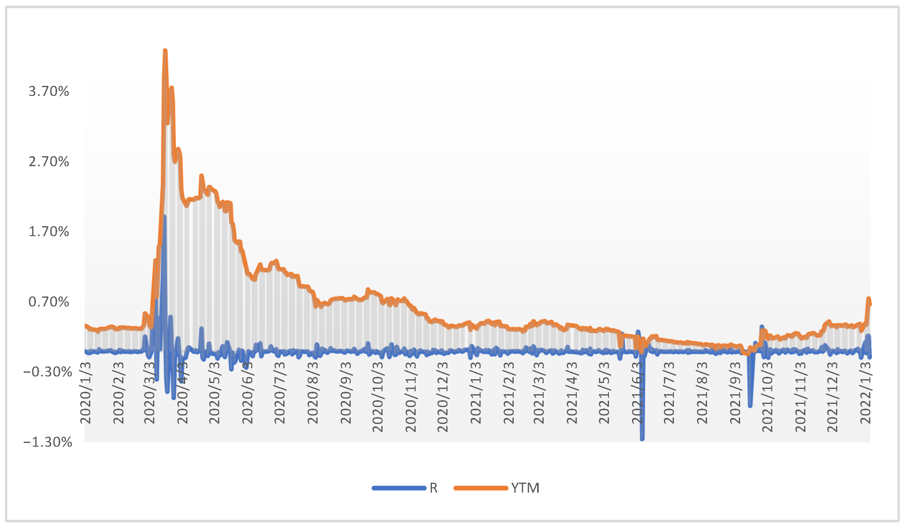
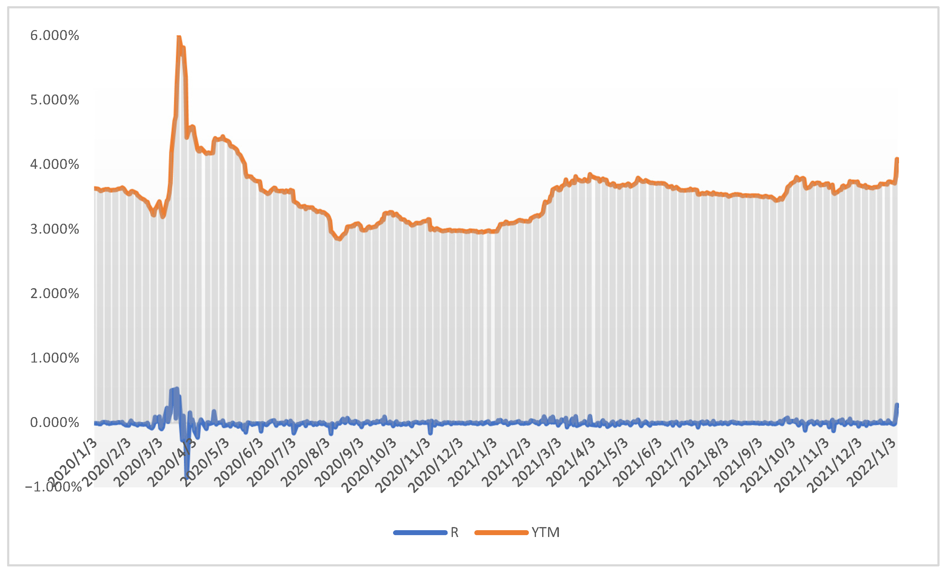
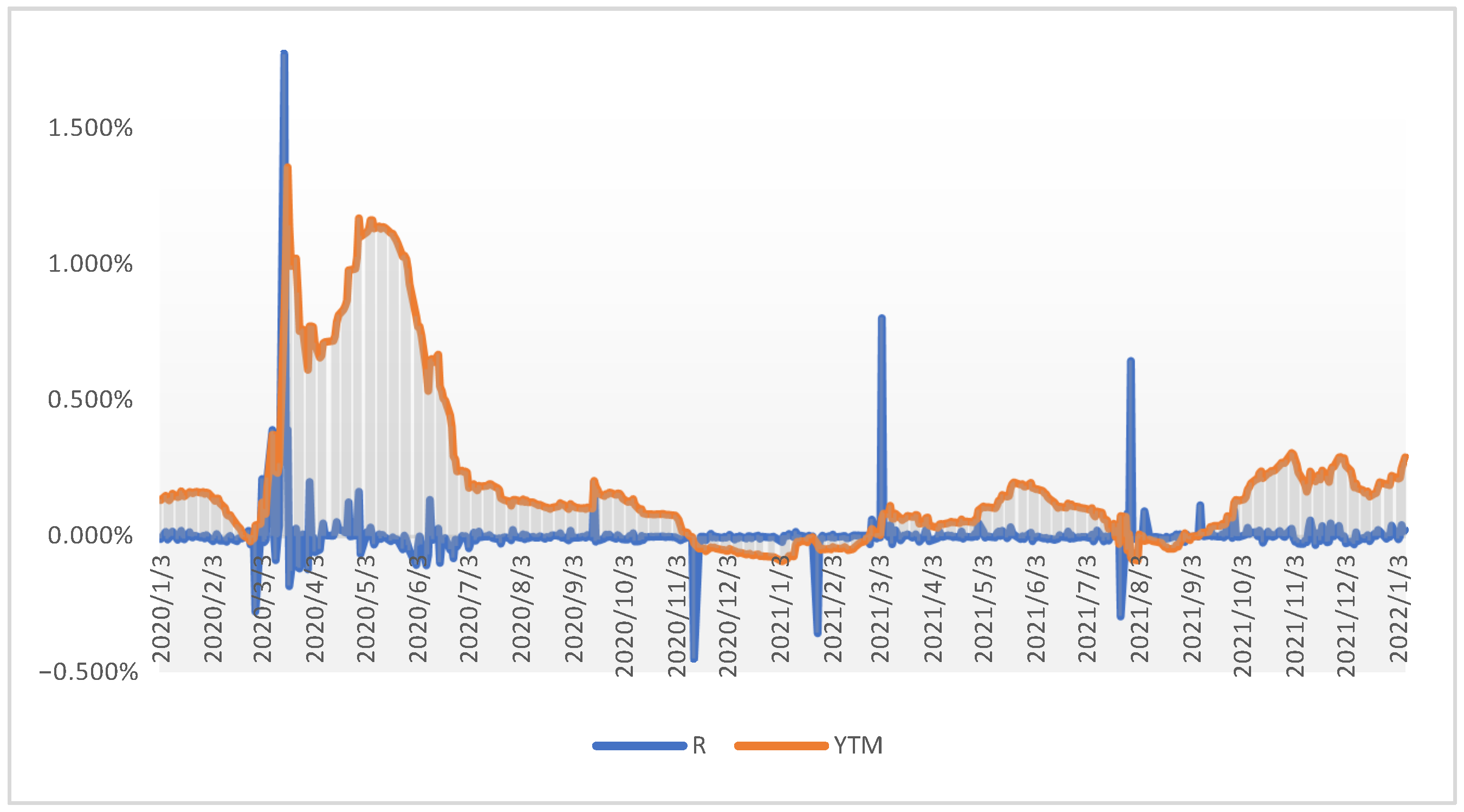
The fourth step is related to the calculation of the yield to maturity according to the following formula:

$$D{P}_i=\left[\frac{FV}{{\left(1+\frac{YT{M}_i}{f}\right)}^{\left(n-1+\frac{DSC}{E}\right)}}\right]+\left[{\displaystyle \sum }_1^n\frac{\frac{C\%}{f}}{{\left(1+\frac{YT{M}_i}{f}\right)}^{\left(n-1+\frac{DSC}{E}\right)}}\right]$$

(2)

where:

• YTMi denotes yield to maturity for a day I;
• DP_i is the clean price for the day I;
• f is the frequency of coupon payment;
• C% is the interest coupon in percent;
• E is the number of days in coupon period in which the settlement date falls;
• DSC is the number of days from the settlement date to the redemption date.

Next, the returns of the yield are calculated as continuous:

$$R_i=ln\left(\frac{YT{M}_i}{YT{M}_{i-1}}\right)$$

(3)

where: R_i denotes the return of yield for the day i.

The sixth step is to calculate the standard deviation of the return according to the following formula:

$${\sigma }_{YTM}=\frac{{{\displaystyle \sum }}_1^n\left(R_i-\overline{R}\right)}{\left(n-1\right)}.YT{M}_n$$

(4)

where:

• $\overline{R}$ denotes the average return of yields;
• ${\sigma }_{YTM}$ is the standard deviation of yield return;
• YTM_n is the last (current) yield to maturity.

The seventh step is the calculation of the modified duration according to the following formula:

$$MD=\frac{1+YTM}{YTM}-\frac{\left(1+YTM\right)+n\left(C-YTM\right)}{C\left({\left(1+YTM\right)}^n-1\right)+YTM}$$

(5)

where: MD_i is the modified duration for the day i.

The specific calculated values of durations and modified durations are presented in Table 11 and Table 13.

The eighth step is calculating the delta normal value at risk for each government bond on a daily basis

$$Va{R}_j=M{D}_i.Z_{\alpha }.\left({\sigma }_Y.YT{M}_n\right).\sqrt{t}$$

(6)

where:

• $Va{R}_j$ is the value at risk for the bond j;
• Z_α is the standardized variable in normal distribution corresponds to probability;
• t denotes investment horizon.

The ninth step is the calculation of delta normal conditional value at risk for each government bond on a daily basis according to the following formula:

$$CVa{R}_j=M{D}_i.{\sigma }_{YTM}\left[-\frac{exp\left[-\frac{{\left(Z_{\alpha }\right)}^2}{2}\right]}{1-\alpha \sqrt{2\pi }}\right]$$

(7)

where:

• $CVa{R}_j$ is the conditional value at risk for the bond j;
• α is a significance level;
• π is a mathematical constant, approximately equal to 3.14159.

The expected shortfall is calculated by averaging all of the returns in the distribution that are worse than the VAR of the portfolio at a given level of confidence.

In the tenth step we calculate VaR, CVaR for 10 days and year by extrapolating according to the following formula:

$$Va{R}_n=Va{R}_d.\sqrt{n}$$

(8)

In the eleven step we calculate undiversified VaR, and undiversified CVaR of the portfolio as the sum of the individual VaR/CvaR values for different time periods. The Undiversified VaR is the sum of individual VaRs, or the VaR portfolio when all assets/yields are perfectly correlated. Accordingly, undiversified CvaR is the sum of all individual CvaRs of bonds.

$$\mathit{Undiversified}\mathit{VaR}={\displaystyle \sum }_{i=1}^n{\mathit{VaR}}_j$$

(9)

Step twelve calculates the correlation matrix of yield’s returns.

Step thirteen is the calculation of diversified VaR of the portfolio according to the following formula:

$$Diversified VaR=\sqrt{{\left(Va{R}_d\right)}^{\prime }Cor.\left(Va{R}_d\right)}$$

(10)

where:

• VaR_d is undiversified daily VaR;
• Cor is YTM return correlation matrix.

Step fourteen calculates the diversified CVaR as follows:

$$Diversified CVaR=\sqrt{{\left(CVa{R}_d\right)}^{\prime }Cor.\left(CVa{R}_d\right)}$$

(11)

where: CVaR_d is undiversified daily CvaR.

Step fifteen is the Sharpe ratio calculation. The Sharpe index is also known as the reward-to-variability ratio. The Sharpe ratio is best used to evaluate portfolios with similar risk characteristics over the same period (Yang 2021). It is calculated for diversified VaR and CvaR by using following formulas:

$$SR\left(VaR\right)=\frac{r_p}{VaR},SR\left(CVaR\right)=\frac{r_p}{CVaR}$$

(12)

5. Conclusions

Market risk is associated with unfavorable price changes in financial or real assets traded on public markets, which cause losses in the investment portfolios of institutional, private, and individual investors. The growing volatility in the price characteristics of the targeted market instruments in recent decades has forced financial managers and academic researchers to concentrate their efforts on improving techniques for forecasting, measuring and managing market risk.

Government bonds are considered one of the lowest risk assets. However, our study shows that in the conditions of the COVID-19 pandemic, the coup attempt in Kazakhstan, and the beginning of the emerging energy crisis, the calculated levels of market risk in the sovereign bond portfolios of Kazakhstan and Bulgaria are relatively high.

Kazakhstan and Bulgaria are two countries, although spatially distant, which show quite similar debt indicators in relative terms in recent years. The market risk research on the government debt of the two countries was limited to the external debt traded on the international financial markets, current as of 8 January 2022 excluding bank loans denominated in different currencies. The study showed that although the two countries may have the same credit rating, approximately the same portfolio duration, similar GDP per capita, Debt (% of GDP), and Debt Per Capita market risk in their portfolio may differ significantly.

The VaR and CVaR values (calculated as Undiversified or Diversified) of the two debt portfolios show differences ranging between 0.55% and 0.8%. This difference is significant because it is calculated daily. It is obvious that despite the extreme events of the coup attempt from the beginning of January 2022, Kazakhstan’s sovereign bond portfolio is much less risky than Bulgaria’s, although the latter is in Europe and is a member of the EU and NATO for more than 15 years.

The portfolio daily difference in Undiversified value at risk (VaR) is 0.7%, in Undiversified conditional value at risk CVaR is 0.8%, Diversified VaR 0.55%, and Diversified CVaR 0.63% in favor of Kazakhstan bond portfolio.

The Sharpe ratio is best used to evaluate portfolios with similar risk characteristics over the same period. The calculated Sharpe ratio values through SR (Diversified VaR), SR (Diversified CVaR) for both portfolios show that Kazakhstan’s sovereign bond portfolio is more than twice (2.19) more efficient than Bulgaria’s bond portfolio.

In the future, the authors intend to study the impact of the ongoing energy crisis on the levels of market risk on sovereign bonds issued on global financial markets by selected European Union countries, as these territorial areas are expected to be most affected.

References

1. Azam, Md. Q., Nazia I. Hashmi, Iqbal T. Hawaldar, Md S. Alam, and Mirza A. Baig. 2022. The COVID-19 Pandemic and Overconfidence Bias: The Case of Cyclical and Defensive Sectors. Risks 10: 56. [Google Scholar] [CrossRef]
2. Basel, II. 2006. Basel Committee on Banking Supervision: International Convergence of Capital Measurement and Capital Standards A Revised Framework Comprehensive Version. Basel: Bank for International Settlements. [Google Scholar]
3. Basel, I. 2016. Basel Committee on Banking Supervision: STANDARDS Minimum Capital Requirements for Market Risk. Basel: Bank for International Settlements. [Google Scholar]
4. Basel. 2019. Basel Committee on Banking Supervision: Minimum Capital Requirements for Market Risk. Basel: Bank for International Settlements. [Google Scholar]
5. Bouri, Elie, Demirer Riza, Gupta Rangan, and Nel Jacobus. 2021. COVID-19 Pandemic and Investor Herding in International Stock Markets. Risks 9: 168. [Google Scholar] [CrossRef]
6. Di Asih, I. Maruddani, and Abdurakhman Abdurakhman. 2021. Delta-Normal Value at Risk Using Exponential Duration with Convexity for Measuring Government Bond Risk. DLSU Business & Economics Review 31: 72–80. [Google Scholar]
7. Fitch Credit Rating Agency. 2022. Rating Report Bulgaria Thu. February 17. Available online: https://www.fitchratings.com/research/sovereigns/bulgaria-17-02-2022 (accessed on 1 March 2022).
8. Giaretta, Elisa, and Giusy Chesini. 2021. The determinants of debt financing: The case of fintech start-ups. Journal of Innovation & Knowledge 6: 268–79. [Google Scholar] [CrossRef]
9. Gong, Qingbin, Zili Tang, and Bing Xu. 2021. Trading behaviors on knowledge of price discovery in futures markets. Journal of Innovation & Knowledge 6: 191–95. [Google Scholar] [CrossRef]
10. Harle, Philipp, Andras Havas, and Hamid Samandari. 2016. The Future of Bank Risk Management; McKinsey Global Institute. Available online: https://www.mckinsey.com/~/media/mckinsey/dotcom/client_service/risk/pdfs/the_future_of_bank_risk_management.pdf (accessed on 3 March 2022).
11. Holton, Glyn A. 2002. History of Value-at-Risk: 1922–1998. Boston: Contingency Analysis Working Paper. [Google Scholar]
12. Jorion, Philippe. 2007. Value-at Risk: The New Benchmark for Managing Financial Risk. New York: McGraw Hill. [Google Scholar]
13. Kazkhstan. 2022. Fitch Ratings Affirms Kazakhstan’s Credit Rating. Retrieved from Official Information Source of the Prime Minister of the Republic of Kazakhstan. April 7. Available online: https://primeminister.kz/en/news/fitch-ratings-kazakstannyn-kredittik-reytingin-rastady-51594 (accessed on 3 March 2022).
14. Krause, Andreas. 2003. Exploring the Limitations of Value at Risk: How Good Is It in Practice? The Journal of Risk Finance 4: 19–28. [Google Scholar] [CrossRef] [Green Version]
15. Lassala, Carlos, Maria Orero-Blat, and Samuel Ribeiro-Navarrete. 2021. The financial performance of listed companies in pursuit of the Sustainable Development Goals (SDG). Economic Research-Ekonomska Istraživanja 34: 427–49. [Google Scholar] [CrossRef]
16. Lee, Michael T., and Ikseon Suh. 2022. Understanding the effects of Environment, Social, and Governance conduct on financial performance: Arguments for a process and integrated modelling approach. Sustainable Technology and Entrepreneurship 1: 100004. [Google Scholar] [CrossRef]
17. Livingston, Miles, and Lei Zhou. 2005. Exponential duration: A more accurate estimation of interest rate risk. Journal of Financial Research 28: 343–61. [Google Scholar] [CrossRef]
18. Mina, Jorge, and Jerry Yi Xiao. 2001. Return to RiskMetrics: The Evolution of a Standard. RiskMetrics Group 1: 1–11. [Google Scholar]
19. Morgan, John Pierpont. 1994. RiskMetricsTM—Technical Document. New York: Morgan Guaranty Trust Company. [Google Scholar]
20. Naseem, Sobia, Muhammad Mohsin, Hui Wang, Liyan Geng, and Kun Penglai. 2021. The Investor Psychology and Stock Market Behavior During the Initial Era of COVID-19: A Study of China, Japan, and the United States. Frontiers in Psychology 12: 626934. [Google Scholar] [CrossRef] [PubMed]
21. Obadovic, Milica, Evica Petrović, Nenad Vunjak, and Mirjana Ilić. 2016. Assessing the accuracy of delta-normal VaR evaluation for Serbian government bond portfolio. Economic Research-Ekonomska Istraživanja 29: 475–84. [Google Scholar] [CrossRef]
22. Samanta, G. P., J. Prithwis, A. Hait, and V. Kumar. 2010. Measuring Market Risk—An Application of Value-at-risk to Select Government Bonds in India. Reserve Bank of India Occasional Papers 31: 1–32. [Google Scholar]
23. Sousa, Joao Beleza. 2012. Bonds Historical Simulation Value at Risk. REM Working Paper Series. Lisboa: Portugal. [Google Scholar]
24. Sousa, João Beleza, Manuel L. Esquível, Raquel M. Gaspar, and Pedro Real. 2014. Historical VaR for bonds—A new approach. Paper present at the 8th Finance Conference of the Portuguese Finance Network, Vilamoura, Portugal, June 16–20; Edited by L. Coelho and R. Peixinho. pp. 1951–70, ISBN 978-989-20-4584. [Google Scholar]
25. Sousa, J. Beleza, Manuel L. Esquível, and Raquel M. Gaspar. 2019. Pulled-to-Par Returns for Zero Coupon Bonds. Historical Simulation Value at Risk. REM–Research in Economics and Mathematics. Lisboa: REM Working Paper 093-2019, ISSN 2184-108X. [Google Scholar]
26. Sun, Yunchuan, Mengyuan Wu, Xiaoping Zeng, and Zihan Peng. 2021. The impact of COVID-19 on the Chinese stock market: Sentimental or substantial? Finance Research Letters 38: 101838. [Google Scholar]
27. Taleb, Nassim. 1997. The world according to Nassim Taleb. Derivatives Strategy 2: 37–40. [Google Scholar]
28. Vlaar, Peter J. G. 2000. Value at risk models for Dutch bond portfolios. Journal of Banking & Finance 24: 1131–54. [Google Scholar] [CrossRef] [Green Version]
29. Yang, Zhou. 2021. Analysis on CAPM and Sharpe Ratio in Market Investment. In Advances in Economics, Business and Management Research, Volume 166 Proceedings of the 6th International Conference on Financial Innovation and Economic Development (ICFIED 2021). Dordrecht: Atlantis Press B.V., pp. 5–8. [Google Scholar] [CrossRef]
Figure 1. The volatility of the yield return and YTM of bond issue Kz18/23 from 2 January 2020 to 8 January 2022. Source: Created by the authors.
Risks 10 00093 g001
Figure 2. The volatility of the yield return and YTM of bond issue Kz15/45 from 2 January 2020 to 8 January 2022.
Risks 10 00093 g002
Figure 3. The volatility of the yield return and YTM of bond issue BG15/27 from 2 January 2020 to 8 January 2022.
Risks 10 00093 g003
Figure 4. Government debt per capita (USD) Kazakhstan vs. Bulgaria. Source: Created by the authors based on data https://countryeconomy.com.
Risks 10 00093 g004
Figure 5. Government debt Bulgaria vs. Kazakhstan (percentage of GDP). Source: Created by the authors based on data https://countryeconomy.com.
Risks 10 00093 g005