The Impact of Health Impairment on Optimal Annuitization for Retirees

Abstract

Post retirement, annuities provide a steady stream of income for retirees. However, the annuitization rate is relatively small in the insurance market in many countries around the world. Prior studies have shown that a substandard health status in retirement reduces annuitization due to adverse selection. Recent innovation introduces an enhanced annuity plan where individuals with impaired health are entitled to higher annuity payments. However, this market is less explored in countries other than the UK. This paper aims to study the optimal annuitization rate where both standard and substandard annuity rates are offered in the market. The life cycle model in this paper incorporates multiple health states based on the likelihood of events and quality of life measures. Our framework consists of two important parts. First, we estimate the transition probabilities of all health states in our Markov model using reliable national data. Second, we derive the optimal consumption and annuitization solution to maximize a retiree’s expected lifetime utility given the uncertainty of future health risk. In addition, we also consider the bequest motive in our optimization problem. Our results show that the optimal annuitization is driven by the choice of bequest and risk-aversion parameters, as well as the health status of the annuitant. Whilst the health-dependent utility parameter only affects our results for certain cases.

1. Introduction

Within the context of retirement, annuities have desirable properties providing a stable stream of income for retirees. Some empirical studies have shown that annuities offer considerably attractive alternatives (in terms of cost and benefit) in many countries (Brown 2002; Fong 2011; Pang and Warshawsky 2010; Turra and Mitchell 2004). Theoretically, the seminal work by Yaari (1965) suggests that full annuitization is optimal assuming the household has no bequest motive. Davidoff et al. (2005) also draw the same conclusion under less strict utility assumptions. However, the voluntary purchase of annuities around the world is low despite the longevity insurance they provide (O’Dea and Sturrock 2019; Alexandrova and Gatzert 2019). This situation is described as an annuity puzzle.

Population aging has been a global phenomenon where individuals with higher than average life expectancy gain the most from annuities through mortality credits. Due to this feature, healthy individuals tend to purchase annuities compared to others with poorer health. Recent innovation has introduced a product called the enhanced annuity, which targets substandard lives (i.e., potential annuitants with medical conditions such as cancer, heart diseases, and hypertension). Generally, the enhanced annuities are different from the standard annuities where additional mortality for individuals with impaired health is taken into account in annuity pricing to overcome the adverse selection issue.

Adverse selection in the annuity market has been the center of many papers in the past. Finkelstein and Poterba (2004) find that adverse selection plays an important role in the annuity market. Brown (2002) identifies adverse selection as one of the explanations for the annuity puzzle. According to Eichenbaum and Peled (1986), for an annuity market that suffers from adverse selection, individuals will choose to accumulate capital privately rather than purchasing annuities that offer higher returns. In a standard annuity, annuity payment does not depend on the potential annuitant’s health state. Thus, enhanced annuities are designed to attract potential annuitants with impaired health to increase the general population’s participation in the annuity market.

Since its inception, this product is popular and continues to surge in the UK having approximately one-third of the UK’s entire annuity market in 2013 (James 2016). The application of this product however requires an extra underwriting process compared to the standard annuity due to the requirement of substandard health proof or medical examination report to determine the entitlement of the product. Nevertheless, according to Ramsay and Oguledo (2020), enhanced annuities clearly offer a fair deal for customers to hedge their longevity risk. The product is expected to thrive further as it offers individuals with impaired longevity the opportunity to receive larger annuity amounts.

Over the past decades, there has been little literature studying the prospect of the annuity market in the least developed countries. According to Park and Shin (2011), owing to the huge increase in the projected old-age dependency ratio from 6% in 1990 to 13% in 2021, retirement costs have continued to increase in recent years, creating a financial burden to future retirees and pension providers. Asher and Bali (2015) underscore the importance of developing a financing mix of pensions in Southeast Asia countries following the World Bank multi-pillars approach which includes a robust annuity market. Thus, there is a growing need to stimulate the annuity market to provide more options for retirees to deploy their retirement resources optimally.

In this article, we consider the optimal annuitization in a market where both standard life annuities and enhanced annuities are offered simultaneously. In particular, annuity pricing depends on the mortality rate of prospective annuitants according to their current health state. Thus enhanced annuity (which is offered to individuals with substandard mortality rates) will be purchased by those with impaired health and standard life annuities will be purchased by healthy individuals. We simulate the results using national data from Malaysia since the enhanced annuity market has never been explored in the country and may have potential demand in the near future. Our model follows the optimal life insurance and annuity purchase model of Fischer (1973) with several extensions.

First, we incorporate several health states over the life cycle of an annuitant using the Markov model and estimate the associated transition probabilities for each state. Second, we apply the health-dependent utility parameter to compare the optimal consumption and annuitization results under the health-dependent and health-independent utility functions optimization model. Third, both standard and enhanced annuities are offered simultaneously so that the annuity price differential reflects fairly based on the current health state of the consumers. In this model, the effect of health dynamics over the life cycle of retirees on optimal consumption and annuitization decision can be captured by allowing single-period (and renewable) term insurance purchase. Hence, it does not allow real long-term annuities purchase. In our experiment, we focus on the retiree’s optimal decision to annuitize or insure overtime during the retirement period depending on his/her current health status rather than one-time annuitization purchase at retirement.

In this paper, we intend to study if consumers’ perception of a particular health status evaluated using the health-dependent utility significantly affects the optimal demand of annuities and consumption patterns. Specifically, we apply the concept of quality of life measure widely used for cost-utility analysis in health economics studies. The idea is to adopt the health index of utility published by the Euroqol group namely the EQ-5D population survey to classify the health status and to calculate the parameter for the health-dependent utility function. To the best of our knowledge, this is the first study that applies this measure in the context of annuity valuation. Therefore, the analysis in this paper provides comprehensive knowledge of the optimal demand of annuities under both utility model preferences to help consumers make a well-informed decision on their retirement plan. In addition, we also study the effect of the bequest motive on the optimal annuitization of consumers under this model setting.

This paper proceeds as follows. Section 2 describes the optimization and the multiple health states model considered in this paper. Section 3 presents the analytical solution to the optimal annuitization and consumption pattern of our model. Section 4 contains the results of the analysis. Lastly, Section 5 concludes.

2. The Optimization Model

The life cycle model in this paper extends the optimal life insurance purchase model in Fischer (1973). Consider an altruistic representative individual who is interested in maximizing his expected utility function by following an optimal nominal consumption path, $C_t$ and a utility attaches to the bequest he leaves, $G_t$. The utility functions are defined in the following iso-elastic form:

$$U\left(h_t,C_t\right)=h_t\frac{C_t{}^{1-\gamma }}{1-\gamma }·\frac{1}{{\left(1+\rho \right)}^{t-1}}$$

$$V\left(G_t\right)={\widehat{b}}_t\frac{G_t{}^{1-\gamma }}{1-\gamma },$$

where $h_t$ denotes the consumer’s health state at time $t,$ $\gamma$ is the risk-aversion parameter, $\rho$ is the rate of time preference, ${\widehat{b}}_t$ is the degree of bequest motive parameter. The function $U\left(h_t,C_t\right)$ captures the utility from consumption and $V\left(G_t\right)$ captures the utility from the bequest. In the utility from the bequest function, the ${\widehat{b}}_t$ factor integrates a discount aspect for the bequest amount leaves in each period $t$. The weighting factor based on health status $h_t$ in this utility function is explained further in Section 2.1. Here, we assume the same risk-aversion level for both functions as in Fischer (1973). By further assuming the consumption utility is additive over time, then the expected utility, denoted by $EU\left(h_t,C_t,G_t\right)$, is defined as follows:

$$EU\left(h_t,C_t,G_t\right)={\displaystyle \sum }_{t=0}^{\omega -x}\left\{{\displaystyle \prod }_{k=0}^t\left(1-q_k^j\right)U_t\left(h_t,C_t\right)+q_{t+1}^j{V}_{t+1}\left(G_{t+1}\right)\right\}$$

(1)

where $q_t^j$ is the probability of death at the beginning of time $t$ which is dependent on the consumer’s current health state $j$, $x$ denotes the current age and $\omega$ is the maximum possible lifespan. In this paper, we deal with single-period (and renewable) term insurance. This model is useful to show the changes in optimal annuitization decisions given the likelihood of health risk as people age. Thus, the representative individual maximizes his expected utility subject to the following budget constraints:

$$W_{t+1}=\left(W_t+Y_t-C_t\right)\left[\left(1-{\alpha }_t\right)R_t\right]$$

(2)

$$W_t\ge 0.$$

(3)

Here $W_t$ denotes the wealth level at time $t$, $Y_t$ denotes the basic annual retirement income if any, $R_t$ is the interest rate factor of $1+i$ at time $t$ and ${\alpha }_t$ denotes the proportion of savings for the insurance premium payment. Positive ${\alpha }_t$ indicates the purchase of life insurance, whilst negative ${\alpha }_t$ means the selling of life insurance or in other words the consumer annuitizes. In this model, the consumer decides the optimal proportion of savings by maximizing his utility preferences. In the event of death of the insured at time $t$, the beneficiaries receive the bequest amount of $G_{t+1}$, which is the sum of remaining wealth and life insurance benefit as follows:

$$G_{t+1}=\left(W_t+Y_t-C_t\right)\left[\left(1-{\alpha }_t\right)R_t+Q_t{\alpha }_t\right]$$

(4)

where $Q_t$ corresponds to the life insurance benefit per dollar premium paid for the insurance plan. Thus, if the proportion of savings for insurance purchase is zero, the beneficiaries will only receive the remaining wealth amount as a bequest. Life insurance is offered at a fair price for both the standard and enhanced life annuities. Hence, insurance is fair when the following equation holds:

$$q_{t+1}^j{Q}_t=R_t$$

(5)

where the interest rate factor $R_t$ is the return on bonds as used in the literature (see, for example, Fong 2011; Mitchell et al. 1999). In this paper, the average rate of return from Malaysian Government Securities is applied as the interest rate factor in our calculation. Since the probability of death depends on the current health state of the consumer at purchase, this factor will distinguish the benefit between the standard and enhanced life annuities. Generally, the life insurance benefit per dollar premium paid is lower for people with impaired health in comparison to healthy individuals due to the higher probability of death for this group. On the other hand, if the consumer decides to annuitize, the annuity is paid at the expense of the life insurance benefit that the beneficiaries have to forgo at a lower amount.

The model that we choose to extend in this paper has nice adaptability to changes or dynamics of health over the life cycle of retirees as they age. Here, the strength of the model is that it allows for the purchase of life insurance or annuity depending on the health state and behavior of the retiree. In our experiment, it is important to study the implication of changes in health status to the annuitization decision over time. The flexibility of making annuitization decisions at any age during retirement shall be one of the possible options in the retirement provision sector to be considered to promote annuities. For example, a retiree may want to convert from an ordinary annuity to an enhanced annuity due to deterioration of health. Thus, this model has been chosen to incorporate the important element of health dynamics in our model.

2.1. Health-Dependent Utility Functions

The consideration of health risk in solving for optimal life cycle consumption and savings has been studied by Ameriks et al. (2011), De Nardi et al. (2010), and Peijnenburg et al. (2015). The utility maximization problem in Peijnenburg et al. (2015) and De Nardi et al. (2010) incorporate health-dependent utility function with two health states, either good ($h_t=1$) or bad health state ($h_t=0$). The utility function is adjusted by a weighting factor based on health status:

$$U\left(C_t,h_t\right)=\left(1+\delta h_t\right)\frac{C_t{}^{1-\gamma }}{1-\gamma }$$

(6)

where the weighting factor $1+\delta h_t$ allows for the effect of health status on the marginal utility of consumption. Thus if $h_t=0$, the health status does not affect utility. The $\delta$ value is chosen meticulously in order to study the effect of health-dependent utility. Both studies apply the isoelastic utility function and find that the health-dependent utility affects the optimal consumption decision though it is not statistically significant.

The health economics study conducted by Levy and Nir (2012) concludes that there is strong empirical evidence supporting the utility of health and consumption and that there exists a trade-off between health and consumption depending on the consumer’s health status. Moreover, according to the empirical data, the logarithmic and isoelastic utility functions can be used as a functional form to capture the trade-off between health and consumption. Consistent with Finkelstein et al. (2013), their results indicate that the marginal utility of consumption declines in poor health. For the case of isoelastic preference, the utility of health and consumption for a consumer currently in health state $h$ is given by1

$$h\frac{C^{1-\gamma }}{1-\gamma }=\frac{{\left[C\left(1-x\right)\right]}^{1-\gamma }}{1-\gamma },$$

(7)

where the left-hand side of the equation is the utility of consumption without treatment and the right-hand side of the equation is the utility of consumption with treatment (perfect health). Note that the right-hand side of the equation assumes that by giving up $x$ proportion of consumption for treatment, the consumer can be fully recovered and hence with perfect health but with lower consumption amount $C\left(1-x\right)$. The formula is derived based on the time trade-off approach that is widely used in the area of health economics to elicit the health index of utility, $h$. Equation (8) also implies that a consumer is indifferent between consuming $C$ in a current health state $h$ or $C\left(1-x\right)$ in a perfect health state.

The empirical study conducted by Levy and Nir (2012) indicates that for less severe conditions (such as diabetes) the health index of utility $h$ is 0.97 (

Table 1. The $h$-value based on the health state.

Health State	$\mathit{h}$-Value
State 1 (Healthy)	1.00
State 2 (Moderate)	0.97
State 3 (Severe)	0.83

). For severe conditions such as cancer, the $h$ value is lower and is found to be 0.83. Thus, we adopt the following values of $h$ in our analysis.

The motivation to introduce the health index measure as the weighting factor for each health status in this model is to explore the implication of applying a more realistic valuation of health state for a particular population based on health economics study. Our analysis will be able to provide more comprehensive knowledge of how retirees should optimally consume and annuitize under both the health-independent and health-dependent utility measures. Previous studies such as De Nardi et al. (2010) and Peijnenburg et al. (2015) have concluded that the implication of health-dependent utility is small, however, the weighting factor of health is not based on the population’s valuation of health status and their model only includes good and bad health state. Here, the life cycle model is expanded to reflect better the life cycle of retirees.

2.2. The Life Cycle Model

The valuation framework in our analysis extends the work of Fischer (1973) by incorporating the possibility of several health states over the life cycle of consumers. Multiple health states Markov model consists of health states namely the healthy, the moderate, and severe impairments to full health, and a dead state.

This multi-state life cycle model is developed to study the implication of having a more realistic life cycle model with various health risks level. If a consumer’s utility of consumption depends on his current health state, allowing for more than one health state in the model could have an impact on our annuity valuation analysis. We use a time-inhomogeneous Markov process in our modeling, where the transition probabilities are age-related and vary over time. Markov model has been extensively applied to quantify the risk associated with health status. For instance, Levantesi and Menzietti (2012) use the Markov model to assess the longevity and disability risk for long-term-care-related insurance.

A multi-state life-cycle model involves determining the number of possible states as well as defining the transition probabilities. For example, Figure 1 depicts a life-cycle model with four well-defined states (i.e., healthy, moderate, severe, and dead) along with ${}_{t}p_x^{i,j}$ which denotes, for a person aged $x$ at time $t,$ the transition probability from state $i$ to state $j.$ The transition probabilities at each time $t$ are more compactly represented by the square transition matrix ${}_{t}p_x$ with dimension equals to the number of states for $t=1, 2, \dots ,T-x$ and $T$ is the maximum lifetime of the consumer. In our application $t$ is typically in the unit of years. We solve for ${}_{t}p_x$ for each time $t$ using matrix multiplication. For instance, to solve for ${}_{2}p_x$, the transition matrix for $t=1$ will be multiplied by the transition matrix for $t=2$; for ${}_{3}p_x$; we then multiply ${}_{2}p_x$ by another transition matrix for $t=3$; and so on. These multiple matrix multiplication tasks are performed using the R software package, where we use the three-dimensional array function as we have three vectors in each transition matrix (a vector for state $i$, state $j$, and age).

The categorization process of these health states within the health impairment model is done by applying the general population EQ-5D survey data published by the Euroqol group consisting of self-reported health status and the associated health index of utility. The Euroqol EQ-5D descriptive system consists of moderate and severe levels of dysfunctions for each of the five dimensions, namely (1) mobility, (2) self-care, (3) usual activities, (4) pain/discomfort, (5) anxiety/depression (MVH 1995). The severity of each dimension has three levels of classification, either (1) no problem, (2) some problem, or (3) severe problem. The EQ-5D health state is then defined as a combination of all five dimensions together with their classifications. Accordingly, state 11111 represents perfect health and state 33333 represents the worst health state. In total there are 243 health possible combinations.

The EQ-5D measure has been extensively used in health economics to evaluate the cost-effectiveness of a particular health-related treatment, often involving the health utility gain over the medical cost spent for a particular treatment through the calculation of Quality-Adjusted Life Years (QALY) (see, for example, Devlin et al. 2020). Another advantage is that this measure has been adopted by many countries to calculate the national index value. Moreover, according to MVH (1995) and Szende et al. (2007), it is a preference-based measure of health-related quality of life most appropriately derived from individual preferences data and has been recommended by several reimbursement authorities and academic bodies in European countries, Canada, and New Zealand. To the best of our knowledge, this is the first study to apply this publicly available measure in developing the multi-state life cycle model.

We seek health outcome prevalence rate data that best reflect our life cycle model from the publicly available EQ-5D related survey. Since Malaysia currently does not have easily available data for estimating transition probabilities of our proposed life cycle model, we resolve this issue by relying on UK’s national data. Specifically, data from the Health Survey for England (HSE) and the Hospital Episode Statistics (HES) are used to estimate the transition probabilities of our life cycle model. This assumption appears to be reasonable in view of the small difference between the UK’s morbidity rates and Malaysia’s morbidity rates (obtained from the Malaysian National Health and Morbidity Survey (NHMS) 2006 (Institute of Public Health 2008))2. The list of EQ-5D values set for the Malaysian population is elicited in Md Yusof et al. (2012)3.

In calculating the transition probabilities of our life cycle model, the risk of longevity is also accounted for. The assumption of a mortality rate for each health state must be made to calculate all other survival probabilities in the model. This is explained further in Appendix A where the derivation of all transition probabilities is presented. Thus, to account for longevity risk, the mortality rate is projected using the Lee-Carter model to allow for mortality improvement factors over time.

$$ln\left(m_{x,t}\right)=a_x+b_x{k}_t+{\epsilon }_{x,t}$$

(8)

where $m_{x,t}$ is the central death rate of age $x$ in year $t$, and the vector $a_x$ can be interpreted as an average age profile of mortality, the vector $k_t$ tracks mortality changes over time, and the vector $b_x$ determines how much each age group changes when $k_t$ changes. These parameters are estimated via the least square approach together with the singular value decomposition (SVD) method (Lee and Carter 1992). The projection is based on the Malaysia mortality rates for the years 1991–2018 obtained from the Department of Statistics, Malaysia (DOSM). We apply the forecast function in R statistical package to estimate the parameters (Hyndman et al. 2022).

3. Analytical Solution to the Optimization Problem

The consumer’s expected utility maximization problem is solved by employing the dynamic programming technique. Assuming that the consumer is in state $j$ at time $T$, the Bellman equation for the final period in our optimization problem is as follows:

$$V_T=\underset{\left\{C_T,{\alpha }_T\right\}}{max}{h}_T\frac{C_T{}^{1-\gamma }}{1-\gamma }+q_{T+1}^j{\widehat{b}}_{T+1}\frac{{\left(W_T+Y_T-C_T\right)}^{1-\gamma }}{1-\gamma }{\left[\left(1-{\alpha }_T\right)R_T+Q_T{\alpha }_T\right]}^{1-\gamma }$$

For the final period, the probability of death equals 1 for all health states. Thus, there is no possibility of surviving beyond time $T+1$. We follow the assumption used in Fischer (1973) that an individual cannot buy life insurance in the final period since death is certain. Thus, the individual does not solve for the optimal life insurance purchase in the final period where ${\alpha }_T=0$. Solving the optimization problem by differentiating the above equation with respect to the decision variable $C_T$, we obtain the first-order condition of the problem as follows:

$$C_T=\left[\frac{{\left(q_{T+1}^j{\widehat{b}}_{T+1}\right)}^{-\frac{1}{\gamma }}{\left(R_T\right)}^{-\frac{\left(1-\gamma \right)}{\gamma }}}{h_T{}^{-\frac{1}{\gamma }}+{\left(q_{T+1}^j{\widehat{b}}_{T+1}\right)}^{-\frac{1}{\gamma }}{\left(R_T\right)}^{-\frac{\left(1-\gamma \right)}{\gamma }}}\right](W_T)$$

(9)

where this solution can be represented as $C_T={\theta }_T^j(W_T)$. Recursively, the Bellman equation for each period can be solved backward. Let us say the consumer is in state 1 at time $T-1$, the following optimization problem is solved:

$$V_{T-1}=\underset{\left\{C_{T-1},{\alpha }_{T-1}\right\}}{max}{h}_{T-1}\frac{C_{T-1}{}^{1-\gamma }}{1-\gamma }+{{\displaystyle \sum }}_{j=1}^3{p}_T^{1j}{h}_T^j\frac{{\left({\theta }_T^j{W}_T\right)}^{1-\gamma }}{\left(1+\rho \right)\left(1-\gamma \right)}+q_T^1{\widehat{b}}_T\frac{{\left(G_T\right)}^{1-\gamma }}{1-\gamma }$$

where $W_T=\left(W_{T-1}-C_{T-1}\right)\left[\left(1-{\alpha }_{T-1}\right)R_{T-1}\right]$ and $G_T=\left(W_{T-1}-C_{T-1}\right)\left[\left(1-{\alpha }_{T-1}\right)R_{T-1}+Q_{T-1}{\alpha }_{T-1}\right]$. If the consumer is in state 2 or 3 at time $T-1$, the second term in the equation above will be adjusted for all possible values of $j$ where transition can occur within the life cycle model. Then, we obtain the following first-order condition for this problem as follows:

$$C_{T-1}=\left[\frac{k_{T-1}{}^{-\frac{1}{\gamma }}}{h_{T-1}{}^{-\frac{1}{\gamma }}+k_{T-1}{}^{-\frac{1}{\gamma }}}\right]\left(W_{T-1}\right)$$

(10)

where

$$k_{T-1}={{\displaystyle \sum }}_{j=1}^3{p}_T^{1j}{h}_T^j{\left(1+\rho \right)}^{-1}{\left({\theta }_T^j\left[1-{\alpha }_{T-1}\right]R_{T-1}\right)}^{1-\gamma }+q_T^1{\widehat{b}}_T{\left(\left[1-{\alpha }_{T-1}\right]R_{T-1}+Q_{T-1}{\alpha }_{T-1}\right)}^{1-\gamma }.$$

Similarly, as the final period, this optimal consumption can be represented as $C_{T-1}={\theta }_{T-1}^1\left(W_{T-1}\right)$ or in general form $C_{T-1}={\theta }_{T-1}^j\left(W_{T-1}\right)$ for $j=1, 2, 3$ depending on the current health state of the consumer. This solution depends on the optimal savings for life insurance purchase ${\alpha }_{T-1}$. Thus, we also solve the optimization problem by differentiating the function with respect to ${\alpha }_{T-1}$. The optimal demand for life insurance/annuity purchase is given below:

$${\alpha }_{T-1}=\frac{R_{T-1}-\beta R_{T-1}}{R_{T-1}+Q_{T-1}\beta -R_{T-1}\beta }$$

(11)

where

$$\beta ={\left[\frac{q_T^j{\widehat{b}}_T\left(Q_{T-1}-R_{T-1}\right)}{{{\displaystyle \sum }}_{j=1}^3{p}_T^{1j}{h}_T^j{\left(1+\rho \right)}^{-1}{R}_{T-1}{\left({\theta }_T^j\right)}^{1-\gamma }}\right]}^{-\frac{1}{\gamma }}.$$

Recursively, the optimal consumption for each period is solved similarly as above. The optimal consumption and annuitization depend on the current health state of the consumer, thus we simulate several scenarios in our model to consider multiple possibilities of health state combinations in our life cycle model.

4. Findings

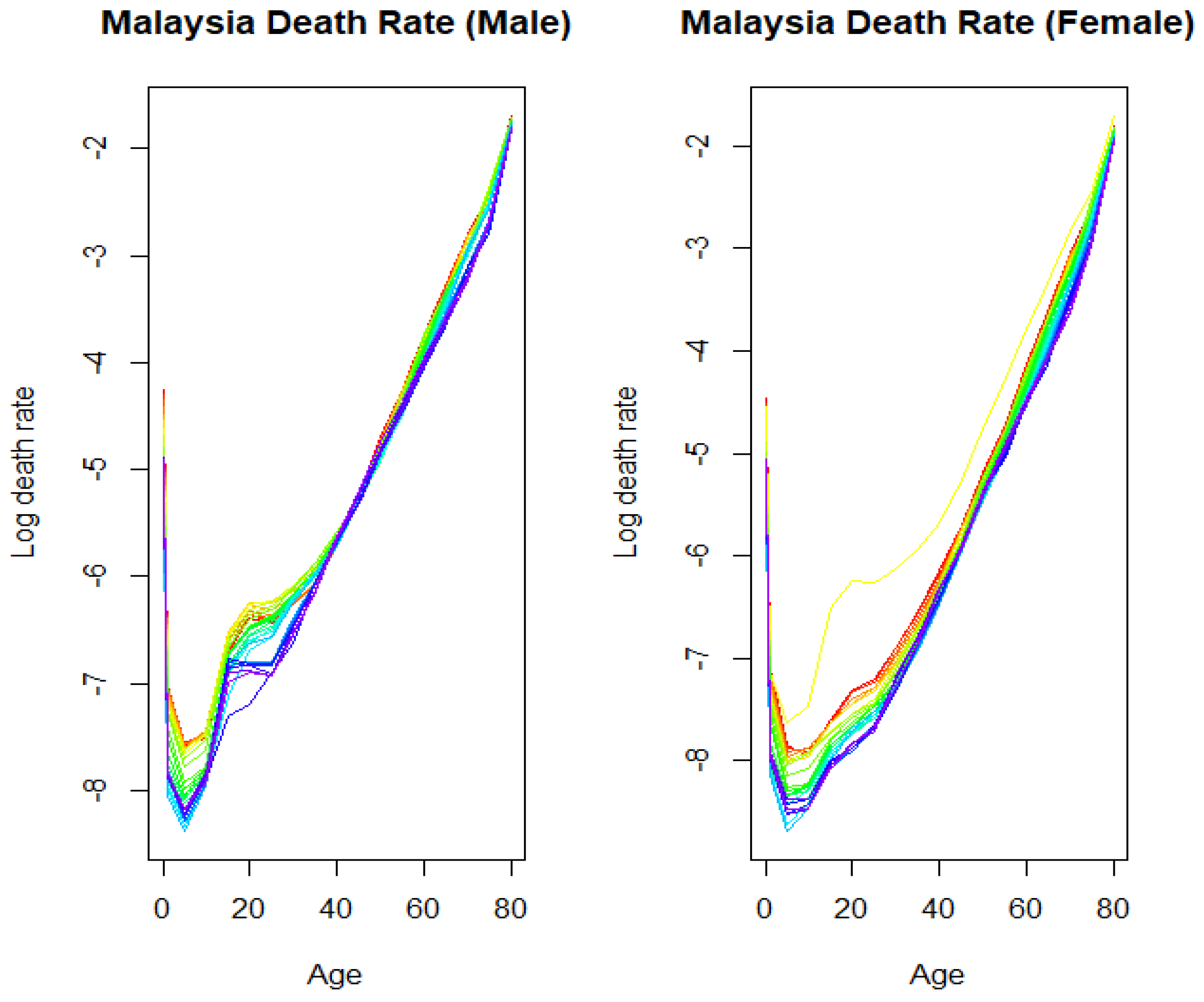
We begin the section by first calibrating the Lee–Carter stochastic mortality model to the mortality curves of Malaysia’s male and female populations from age 0 to 80 over the entire period from 1991 until 2018. The results are depicted in Figure 2, with the years labeled using the rainbow plots. The earliest year is presented by the first color of the rainbow (red) corresponds to the earliest year while the last color of the rainbow (violet) corresponds to the latest year.

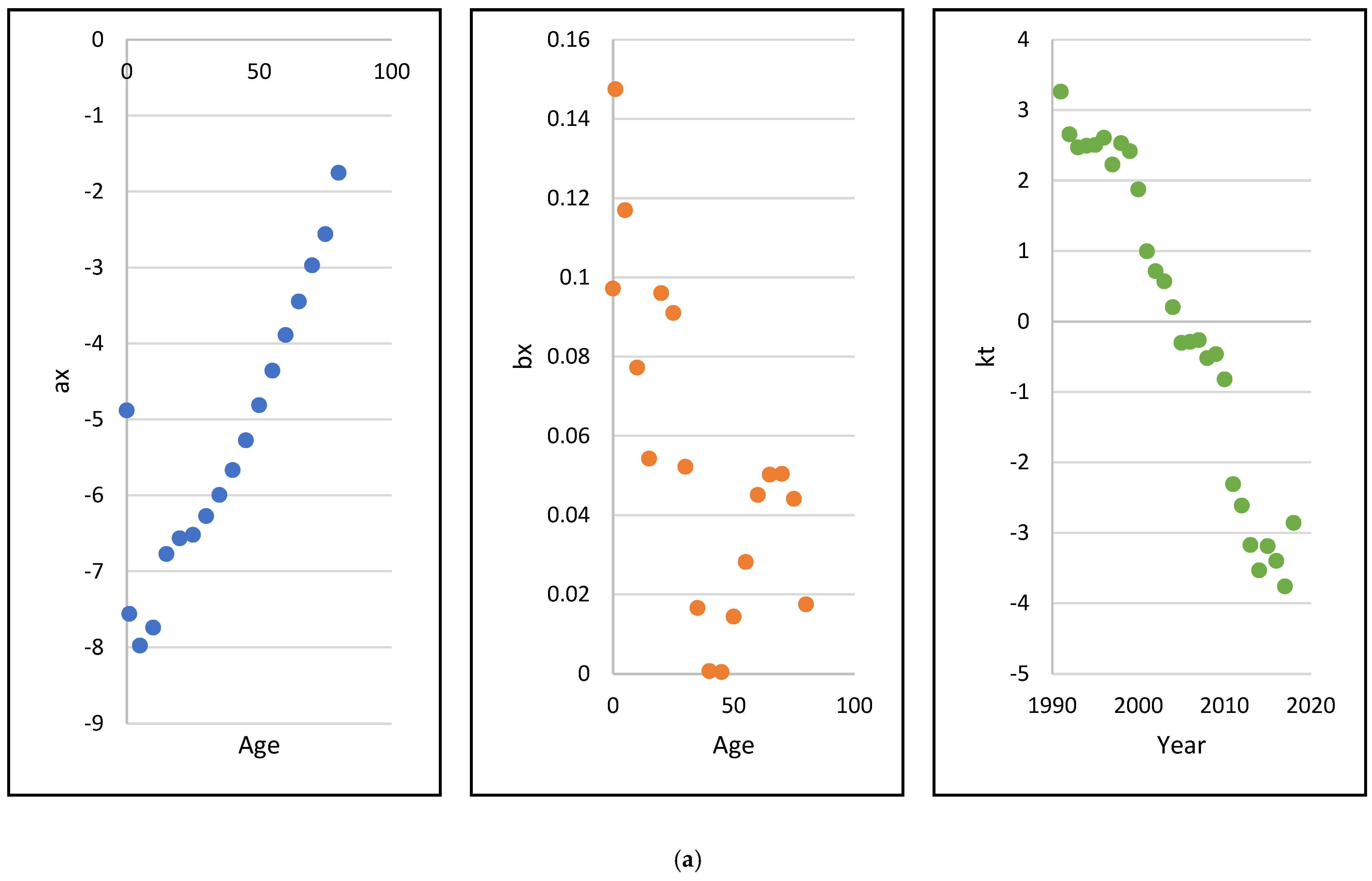
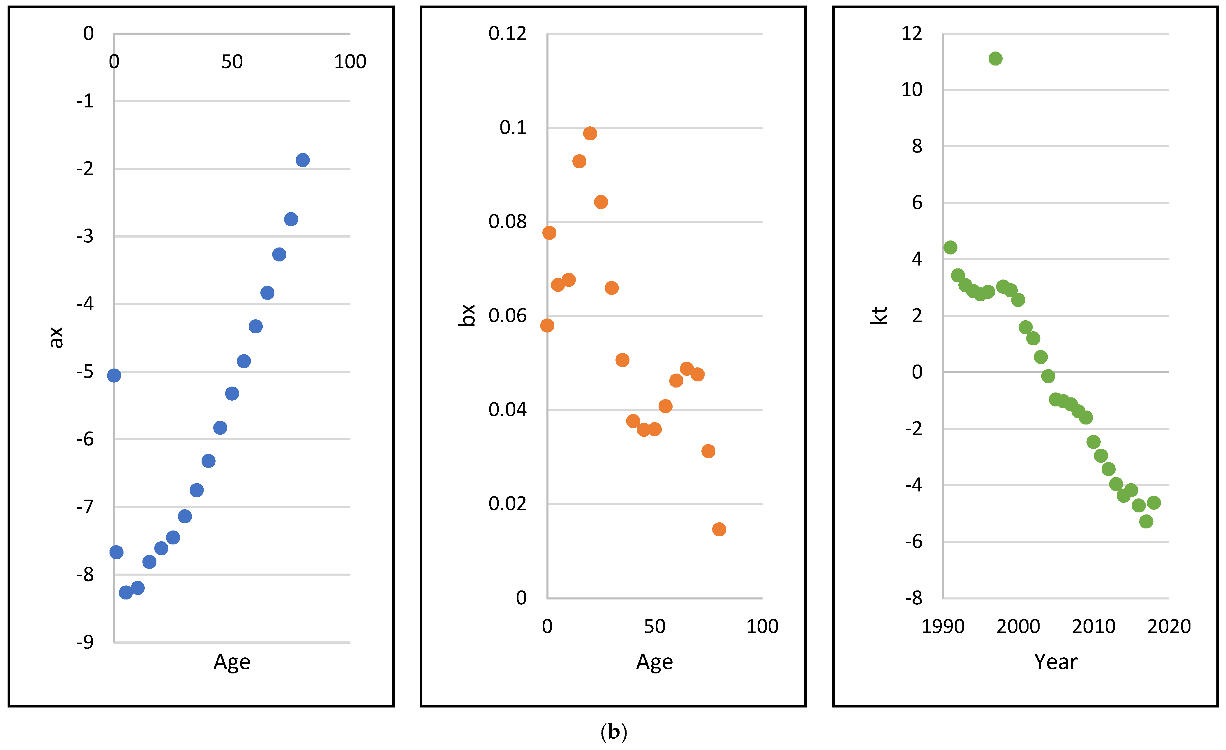
The estimated Lee–Carter parameter values $(a_x,$ $b_x,$ $k_t)$ for males and females are shown in Panels (a) and (b) of Figure 3. Beyond a certain critical age (around age 10) the estimated ${\alpha }_x$’s for both genders are increasing implying an upward trend in mortality as age increases while the estimated $b_x$’s are oscillating with a downward trend. The estimated $k_t$’s, which capture the pattern of mortality over time, indicate decreasing mortality rates over the period of 1991 to 2018.

4.1. Optimal Annuitization Results

The analysis is conducted for the Malaysian population aged 60 at retirement, for both males and females. The starting wealth amount is set at MYR316,339 (MYR is Malaysian Ringgit, the currency of Malaysia), which is the average balance of the Employees Provident Fund for private-sector employees in Malaysia prior to retirement extracted from the Employees Provident Fund Annual Report 2018 (Employees Provident Fund 2018). Several scenarios are simulated based on the possible combination of health states that can occur over the consumer’s life cycle. These scenarios are outlined as follows:

• Scenario 1: The consumer stays healthy until the maximum lifetime.
• Scenario 2: The consumer stays in the moderately impaired health state until the maximum lifetime.
• Scenario 3: The consumer stays in the severely impaired health state until the maximum lifetime.
• Scenario 4: The consumer’s health deteriorates over time (10 years in the healthy state, then transits to the moderate state for 20 years, and finally transits to the severe state thereafter).
• Scenario 5: The consumer’s health status improves over time (initially 20 years in the moderate state and then transits to the healthy state thereafter).

The above scenarios are selected to enhance our understanding of the impact of the consumer’s health status dynamic on the pattern of optimal annuitization/insurance purchase. For risk-aversion and bequest level parameters, we assume in our analysis that they can take two possible values, depending on “low” rates or “high” rates. Their respective values are shown in

Table 2. The Parameter Values for the Optimization Model.

	Assumption
Parameter	Low	High
Risk-aversion, $\gamma$	0.85	0.99
Bequest level, ${\widehat{b}}_t$	0.80	0.90

.

To further compare and contrast the role of health on annuitization/insurance purchase, we divide our analysis into two cases with utility functions depending and not depending on health. For each case, we consider four possible combinations of risk-aversion and bequest level parameters; that is, (a) low risk-aversion, low bequest level; (b) low risk-aversion, high bequest level; (c) high risk-aversion, low bequest level; (d) high risk-aversion, high bequest level.

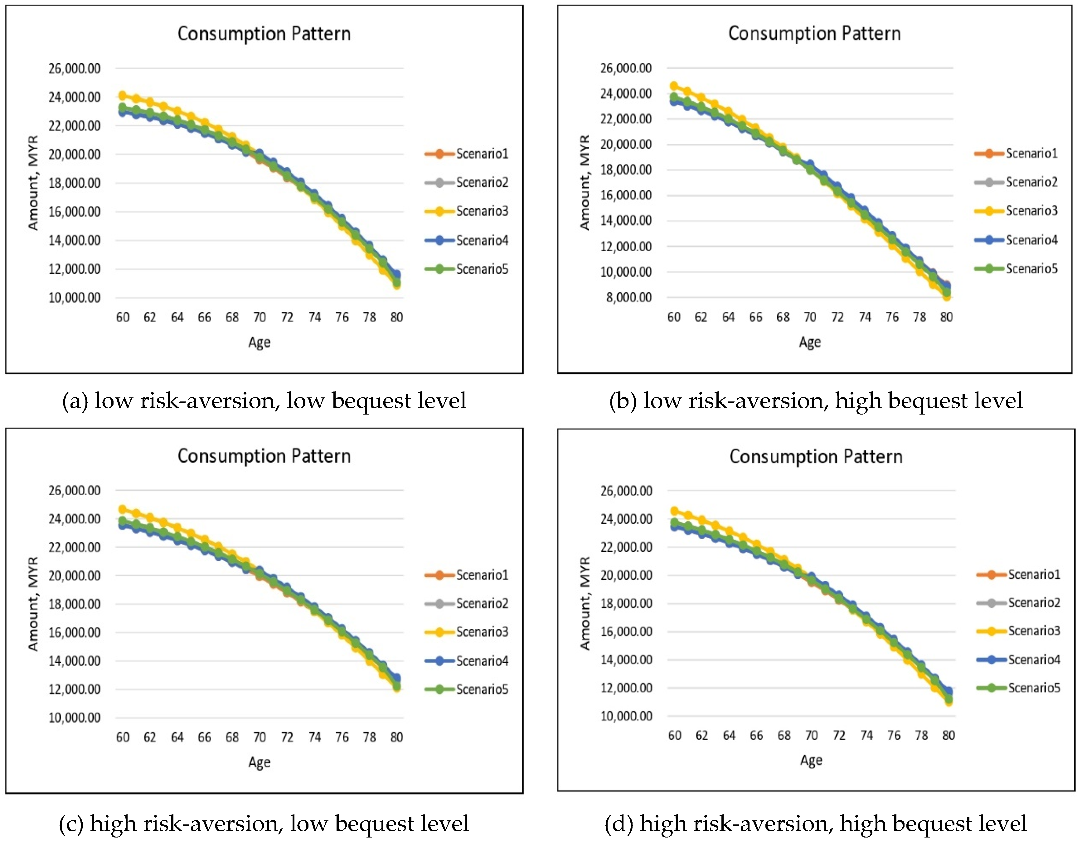
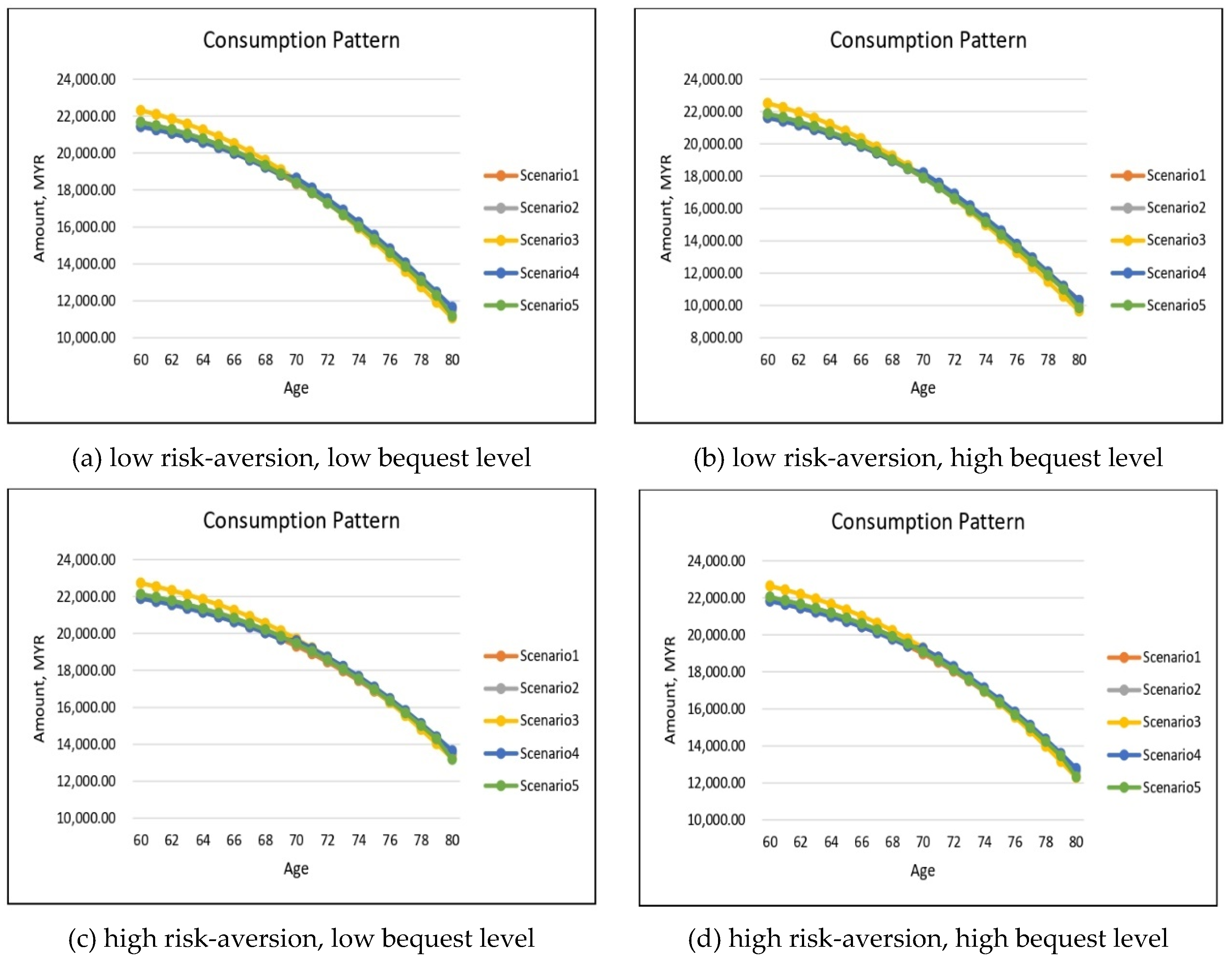
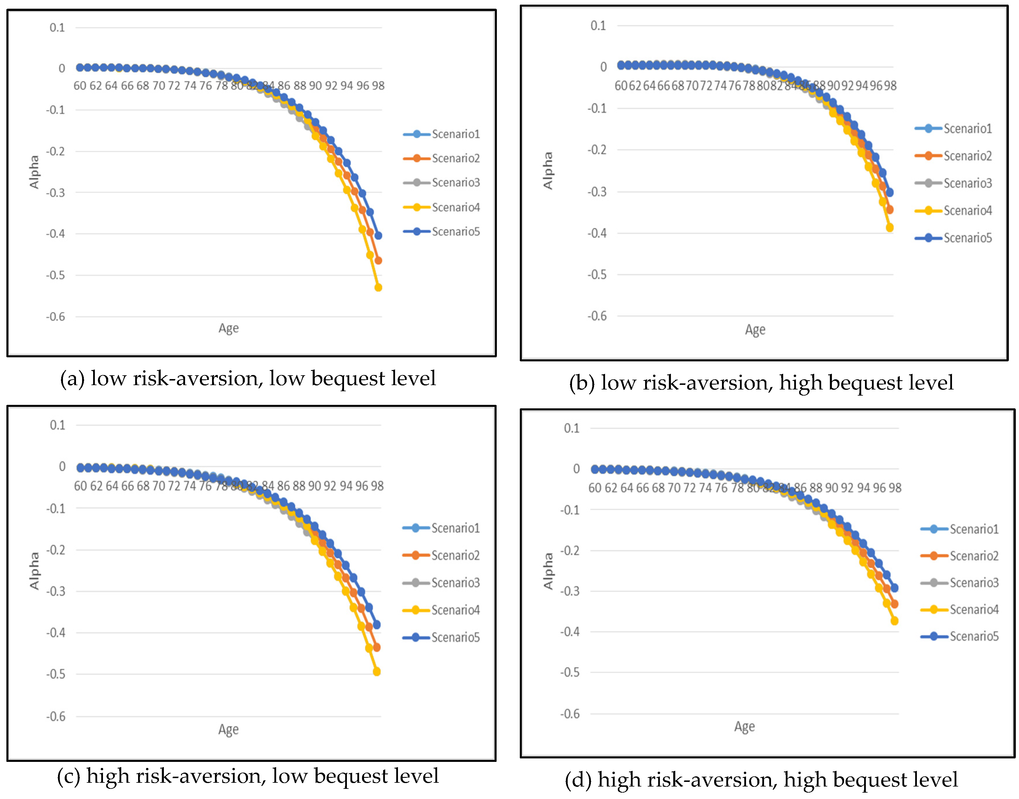
For the health-independent utility case, this can be achieved by merely setting the health index of utility to 1 regardless of health state. Under all five considered health scenarios, the simulated optimal consumptions for males and females are presented in Figure 4 and Figure 5, respectively. Figure 6 and Figure 7 show the optimal results but for annuitization/insurance purchase. Without health-dependent parameters, the optimal consumption paths appear to have similar patterns for all five health scenarios with an exception for Scenario 3 where the severely impaired individual consumes slightly higher in the early years of retirement in comparison to other health scenarios. In addition, there is a noticeable difference in the optimal consumption amount depending on the risk-aversion and bequest level parameters, particularly as the retiree ages.

The effect of risk-aversion on optimal consumption can be inferred by comparing panel (a) with panel (c) and panel (b) with panel (d) for both genders. Note that for each pair of comparisons, the bequest level parameter is held constant but the risk-aversion parameter changes. The lower risk-aversion cases (i.e., (a) and (b)) exhibit quite similar starting value of consumption amount in comparison to the higher risk-aversion case (i.e., (c) and (d)), but as the retiree ages reaching the age of 80, the consumption amount for low risk-aversion case is significantly lower than the high risk-aversion case. This indicates that the increase in the risk-aversion parameter has resulted in higher consumption in the later years of retirement which shows that more risk-averse individuals prefer to smooth out their consumption. This is also due to the fact that more risk-averse individuals tend to annuitize earlier at the age of 60 while less risk-averse individuals start to annuitize at a later age around 70–80. The less risk-averse individuals will in fact choose to purchase a small amount of life insurance in the early years of retirement as shown in Figure 6 and Figure 7 (refer to Appendix B-Figure A1 for a clearer illustration of this life insurance purchase).

If the risk-aversion parameter is held constant and if a consumer wishes to increase the level of the bequest to his/her beneficiaries, the optimal consumption exhibits a similar pattern except for the case of low risk-aversion and high bequest level as shown in Figure 4 and Figure 5 (panel (b)) where the consumption level is significantly lower reaching age 80 in comparison to other parameter combinations (panels (a), (c) and (d)). The increase in bequest level also has more of an effect on the insurance purchase decision, as confirmed in Figure 6 and Figure 7 by comparing panel (a) with panel (b) and panel (c) with panel (d) for both genders.

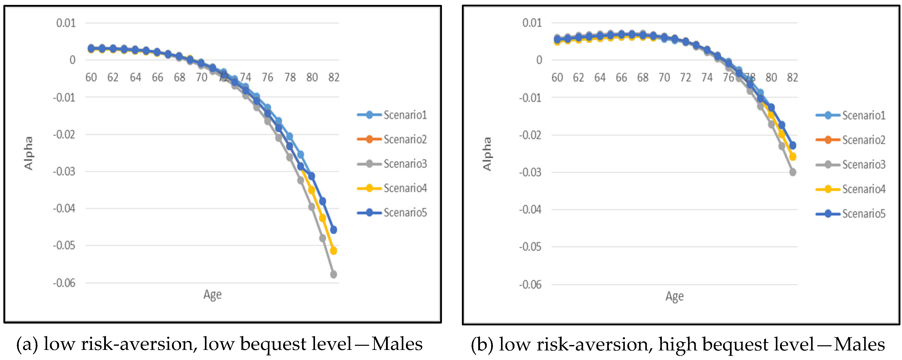
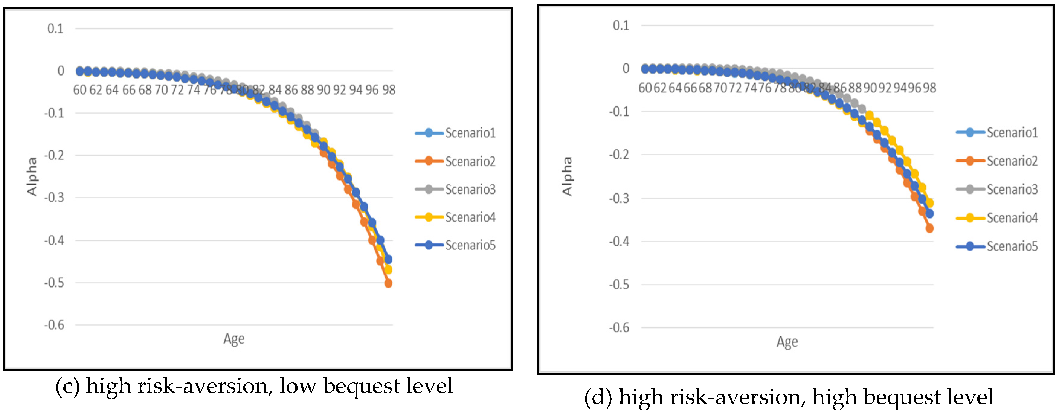
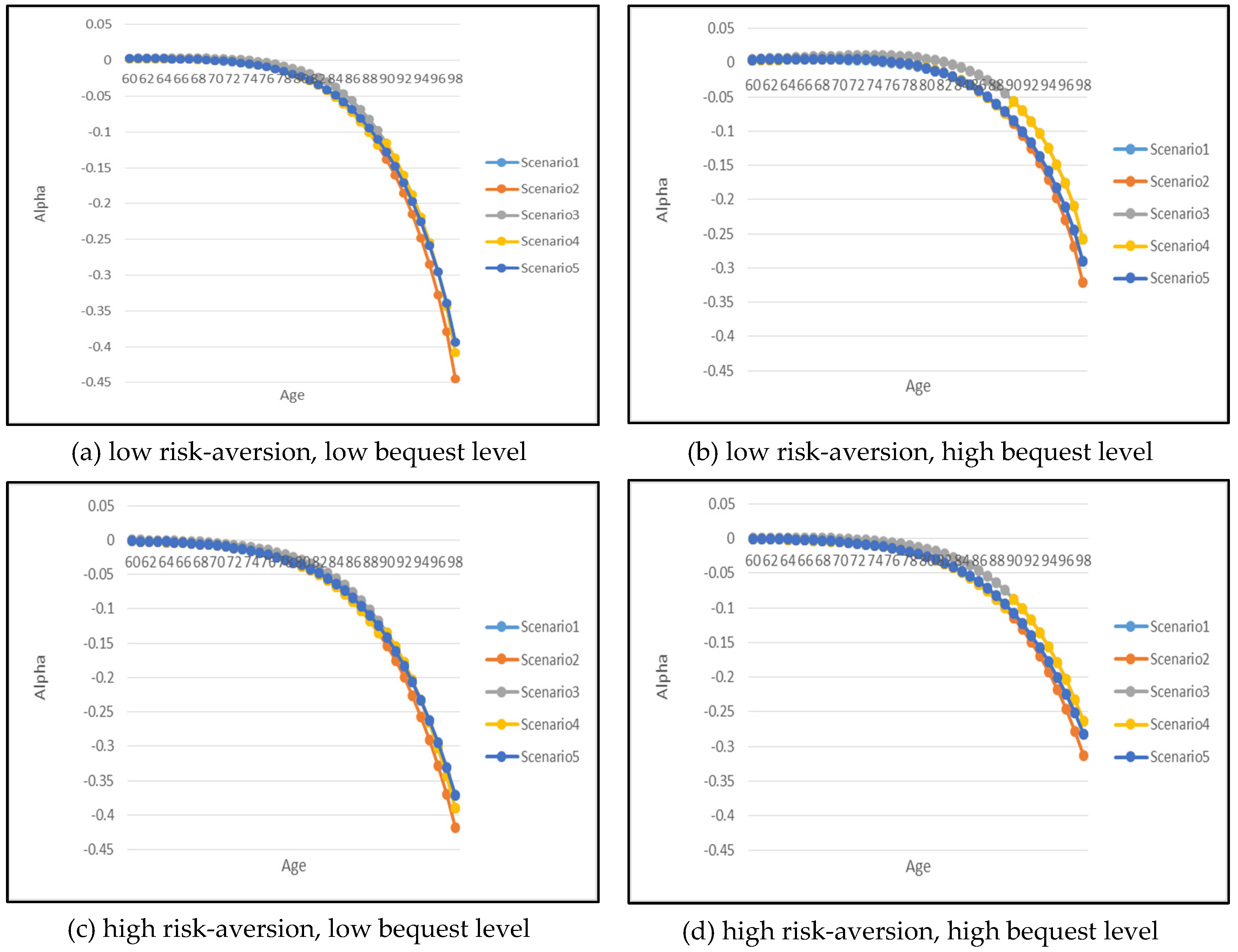
Let us now analyze the optimal annuitization/insurance purchase. Recall that positive $\alpha$ indicates the proportion of current wealth spent on life insurance purchase while negative $\alpha$ implies annuity purchase. Generally speaking, the demand for optimal annuitization increases with age. Also as risk-aversion increases, there is a greater reliance and greater demand on annuity where retirees choose to annuitize in the early years of retirement. A low risk-aversion and high-bequest retiree produces an interesting phenomenon. As shown in panel (b), it is optimal for the retiree to support a higher level of bequest via life insurance purchase in the early years. As the retiree ages beyond 76 years old, it is then optimal to start annuitizing their wealth.

Figure 6 and Figure 7 also show that the demand for annuitization/insurance depends on the health scenario, especially at old age. For example, it is of interest to note that as a retiree’s health improves over time (i.e., Scenario 5), the demand for annuitization is the lowest. In contrast, when the retiree’s health deteriorates over time (i.e., Scenario 4), the demand for annuitization is the most, with the difference in demand progressively more pronounced for ages beyond 80 years old.

For gender differences, the demand for annuitization is higher for males in comparison to females for all combination of parameters, which is mainly due to higher mortality rates that contribute to much cheaper annuity price for males.

4.2. The Implication of Health-Dependent Utility Function

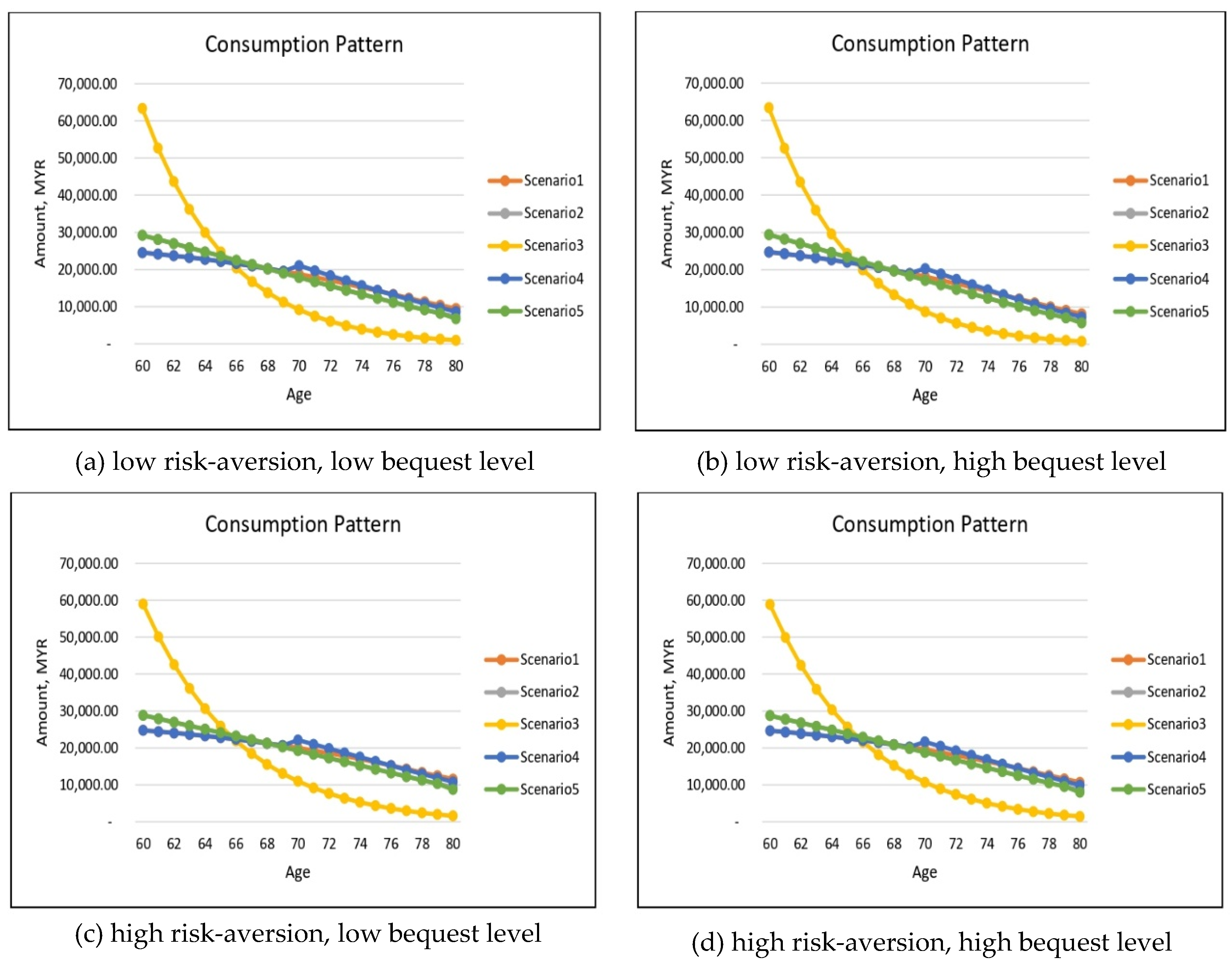
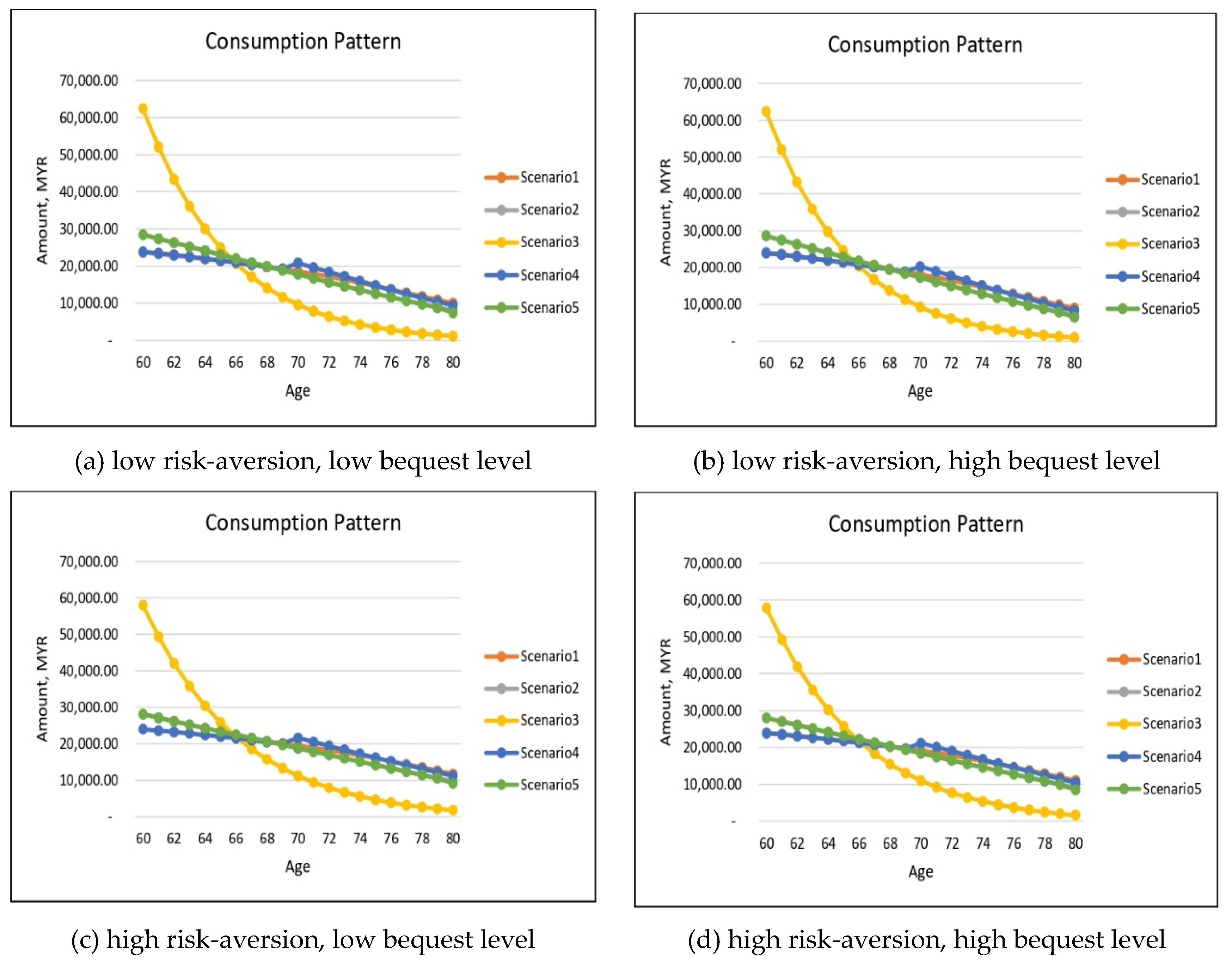
We now turn to our empirical analysis toward the health-dependent utility function by varying the health index of utility $h$ as a function of health status as according to Table 1. Figure 8 and Figure 9 provide the simulated results for the optimal consumption for both males and females except for the health-dependent utility function. In general, the impacts of risk-aversion and the level of bequest on optimal consumption for the health-dependent utility function optimization model are similar to the optimization model with a health-independent utility function. For example, increasing risk-aversion induces greater later consumption reaching age 80, as also noted in the health-independent utility function though the difference is less pronounced.

When there is no health differential in utility value, we have previously concluded that the optimal consumption patterns are very similar for our five health scenarios with a slightly higher consumption at early retirement for severely impaired individuals (see Figure 4 and Figure 5). There is, however, a striking difference when a penalty is imposed on substandard lives. This is highlighted in Scenario 3 with the retiree remaining in the severely impaired health state throughout. This phenomenon applies to both genders and to all combinations of risk-aversion and bequest levels. The significantly large consumption amount in the early years of retirement is to be expected in view of the retiree’s severely impaired health; because of low chances of recovery and/or surviving to older ages, it would be optimal for the retiree to consume more earlier while still alive. This is also consistent with our findings for the health-independent utility model, but to a lesser degree. The higher demand for substandard retirees may be induced by the lower cost of annuitization.

Finally, let us focus on the optimal annuitization/insurance purchase under the health-dependent utility optimization model. The necessary results are summarized in Figure 10 and Figure 11 for males and females respectively. Similarly to our findings for the health-independent utility model, retirees should optimally annuitize under panels (a), (c) and (d) and for panel (b) with low risk-aversion and high bequest level, the insurance purchase will ultimately dominate the early years of retirement period to support the desire to leave a higher level of bequest for the beneficiaries.

Recall that for annuitization Scenario 4 has the highest demand while Scenario 5 has the lowest for the health-independent utility model. For the health-dependent utility model, Scenario 2 with the retiree staying in the moderately impaired health state will annuitize the most. This is contrary to the findings in the health-independent utility model setting where severely impaired individuals annuitize the most. Thus, we can conclude that if individuals value their current health state differently, this will also affect their optimal annuitization/insurance purchase decision.

In this case, there is a trade-off between the cheapest annuity price offered under the enhanced annuity for the severely impaired individuals and how the individual values the extra consumption received from the annuity payment, given his/her current health state. Nonetheless, for individuals with low bequest motive, as depicted in panels (a) and (c), the severely impaired individuals still annuitize at a rate close to the moderately impaired individuals’ annuitization rate.

In summary, the optimal annuitization amount decision depends on the individual’s risk-aversion parameter, bequest parameter, and also his/her current health state. While the consumption pattern does not vary much by health state if the individual values all health states indifferently as shown in the health-independent utility model setting. Our analysis helps to understand how retirees should annuitize based on his/her risk-aversion and bequest level. Most importantly, opening a fair annuity market for individuals with substandard health will increase the optimal annuitization amount amongst retirees. Thus, the enhanced annuity market potentially reduces the problem of adverse selection for annuity providers.

5. Conclusions

Despite annuities being known for their desirable properties, the world’s voluntary annuitization rate is low. This situation, described as the annuity puzzle, has drawn the attention of policymakers, insurers, and researchers working on potential future retirement fund alternatives. Recent innovations in retirement products include the introduction of enhanced annuities. This product is less explored in the market other than in the UK. Hence, there is a lack of understanding of how future retirees should value the benefit offered under this product.

This paper extends the optimization model in Fischer (1973) by including several health states in the consumer’s life cycle to study the optimal demand of both the standard and enhanced annuity market. We find that individuals with substandard health should optimally annuitize more if the annuity is fairly priced based on their substandard mortality rates. On the other hand, individuals will insure instead if their desire to leave a bequest is very high.

This study also contributes to the literature in providing further justification of how people’s perception toward future health risks could affect their annuitization decision. Even though a fair annuity market is available, our findings indicate that under the health-dependent utility optimization model, the optimal annuitization amount reduces for someone with a severe health condition because the individual values his consumption significantly lower in comparison to the consumption in a healthy state. However, the annuity purchase amount is still significant under both the health-dependent and health-independent utility optimization model. This underscores the potential demand for enhanced annuities in structuring better future retirement plans.