Role of the Global Volatility Indices in Predicting the Volatility Index of the Indian Economy

Abstract

Movements in the volatility index of the Indian economy are influenced by global volatility indices (fear index). This study evaluates the influence of various global implied volatility indices in forecasting the day-to-day binary movements in the implied volatility index of India, denoted by the symbol ‘India VIX’. Historical daily data from 18 September, 2009, to 2 December, 2021, was acquired, and the target labels were created from changes in the India VIX. A set of classifiers, consisting of Logistic Regression, Random Forest and Extreme Gradient Boosting (XG Boost), were applied to rank the feature variables according to their importance. This study revealed that India’s VIX was impacted most by the previous day’s changes in the closing value of the US implied volatility indices, except for the Chicago Board Options Exchange (CBOE) Eurocurrency volatility index. Additionally, the Eurozone implied volatility index was also important. However, the implied volatility indices of Australian Hang Seng and Japan were the least important. This study’s outcomes help Indian traders in creating a watch list of important volatility indices.

1. Introduction

Risk fluctuates across time. It increases as volatility increases, such as in times of a pandemic or a financial crisis. There are many examples, such as the Great Depression in 1929, the sub-prime crisis from 2008 to 2010, COVID-19 in 2020 and the very recent Ukraine–Russia War, during which huge volatility is seen due to the fear factor. The implied volatility index of the Indian stock market is denoted as ticker ‘India VIX’, while the implied volatility index of the Chicago Board Options Exchange (CBOE) is denoted as ‘CBOE VIX’ or ‘VIX’.

The VIX Index is the implied volatility of options prices written on the underlying index and the most important risk indicator in the stock market. For the CBOE VIX Index, the underlying index is the S&P 500 Index (SPX), and for the India VIX Index, the underlying index is the Nifty 50 Index. Changes in the volatility index suggest how perceptions change across time and are an essential tool for investment risk management. Some researchers (Carr 2017; Onan et al. 2014; Sarwar 2012) believe that VIX is a fear index, while others (Bantwa 2017; Chandra and Thenmozhi 2015) propose a risk hedging technique.

In 1993, CBOE Global Markets announced the CBOE Volatility Index, denoted as ticker ‘VIX’. It was initially constructed to assess the 30-day market’s anticipation, based on the implied volatility of the at-the-money options trading at the S&P 100 Index. It was later updated, in 2003, to incorporate a new methodology to measure the expected implied volatility of the S&P 500 Index options. This new volatility index computes anticipated volatility by gathering the weighted prices of the SPX calls and puts options over a wide range of strike prices.

The India VIX was created by the National Stock Exchange (NSE) of India, in 2008, and is based on the prices of the Nifty 50 Index options. It uses the same construction methodology (India VIX White Paper 2008) as that of the CBOE VIX Index (CBOE VIX White Paper 2003), licensed from CBOE. While some of the implied volatility indices are computed by the methodology standardised by the CBOE, other implied volatility indices outlined by Siriopoulos and Fassas (2013) are still computed using the Black–Scholes–Merton formula, derived by Black and Scholes (1973) and Merton (1973).

A high level of VIX creates uncertainty, and a low level of VIX builds confidence in the stock market. Some researchers (Bantwa 2017; Chandra and Thenmozhi 2015) highlighted that the implied volatility index and its underlying index move in opposite directions, and that this opposite movement is even stronger when the market is moving in a downward direction. Other researchers (Onan et al. 2014; Sarwar 2012) revealed that a high level of the VIX Index negatively influences the global stock market in addition to the US stock market. It could be seen during the sub-prime crisis in 2008 and 2009 and the COVID-19 catastrophe in 2020 that the implied volatility index rose sharply and stock markets bled. Such trends were also observed when adverse news spread throughout the world. For example, when news about Omicron, a variant of COVID-19, broke out in South Africa on 26 November 2021, there was a sharp upward spike in implied volatility indices and the stock market significantly decreased, as shown in

Table 1. Change in implied volatility indices due to the news of Omicron.

Change in Volatility Index	24 November 2021	25 November 2021	26 November 2021	29 November 2021	30 November 2021
Delta_INDIAVIX	−0.920	−0.433	4.140	0.028	0.338
Delta_VIX	−0.800	−0.800	10.040	−5.660	4.230
Delta_OVX	−0.310	−0.310	30.930	−2.380	11.890
Delta_VXN	−0.610	−0.610	4.630	−3.820	2.760
Delta_EVZ	−0.260	−0.260	0.590	−0.420	0.430
Delta_VVIX	−4.550	−4.550	39.260	−18.500	11.310
Delta_GVZ	−0.060	−0.060	1.240	−0.440	0.440
Delta_RVX	−0.480	−0.480	13.170	−6.020	3.560
Delta_VXD	−0.360	−0.360	6.990	−1.710	3.440
Delta_VHSI	−0.430	−0.660	4.520	1.040	−0.670
Delta_JNIV	0.860	−0.530	3.320	5.000	1.800
Delta_AXVI	−0.324	−0.758	1.695	2.264	−1.051
Delta_VSTOXX	0.030	−0.790	12.430	−3.510	1.270

Note: Data is taken from respective indices from 24 November 2021 to 30 November 2021. Delta indicates a change in the closing value of the given tickers over a day. Table 2 can be referred for Tickers.

.

Stock markets of China, Japan, the US, and the UK influence the Indian market (Tripathi and Sethi 2010). Foreign Institutional Investments (FIIs) impact the Indian stock market (Kapoor and Sachan 2015; Nandy and Chattopadhyay 2019). The BRICS stock market has a significantly volatile spill-over effect from the US stock market (Bhuyan et al. 2016) and is dependent on the global stock and commodity market, and, more importantly, on the CBOE VIX Index (Mensi et al. 2014).

Considering the vulnerability of the Indian stock market to the global market, it is important to examine the influence of the global implied volatility indices on the Indian volatility index. Generally, Indian traders keep their eyes only on the India VIX, but it would be a better idea if Indian traders kept their eyes on the global volatility indices, so that the multidimensional risk in the Indian market is anticipated. This study’s outcomes are an important tool for investors and traders of Indian economies in anticipating the risk level in their local stock market. Ultimately, it provides a set watch list of implied volatility indices for traders and investors of Indian economies.

To anticipate feature variables’ influencing powers, a classification problem was constructed, and to build the classification model, a standard classifier, called Logistic Regression, and advanced classifiers, called Random Forest and Extreme Gradient Boosting (XG Boost), were applied. Logistic Regression (Aliyeva 2021, August; Zhang et al. 2022) helps detect directional relationships. Random Forest (Sadorsky 2021) and XGBoost (Wang and Guo 2020; Vuong et al. 2022; Han et al. 2023) were applied because, like stock market forecasting, VIX forecasting is a time-series forecasting in which variables reveal temporal dependencies and the relationship is likely to be non-linear.

In the next section, past studies consisting of implied volatility indices, feature importance and a few machine learning techniques are reviewed. Subsequently, the research design and methodology are discussed, and the outcome of the findings is analysed. Finally, the study’s findings are concluded.

2. Literature Review

By employing a dynamic conditional correlation (Engle 2002; Chaudhary et al. 2020a); Siriopoulos and Fassas (2013) investigated spill-over impacts in the international financial market with respect to publicly available implied volatility indices. Their outcomes indicate a strong integration of investors’ expectations about future uncertainty. Additionally, conditional correlations of market expectations change over the horizon. The conditional correlations of all reviewed implied volatilities only slightly increased over the years. Conditional correlations across implied volatility indices increase during a panic-like situation in the market.

Shaikh and Padhi (2014) compared the prediction accuracy of ex-ante, ex-post and volatility predictions to realise the return volatility of different periods. The implied volatility, GJR-GARCH (Glosten-Jagannathan-Runkle Generalized AutoRegressive Conditional Heteroskedasticity), and RiskMetrics competed in volatility forecasts. Their results revealed that implied volatility was predominant, and that ex-ante volatility was best for describing upcoming market volatility with in-sample forecasting. For the non-overlapping sampling procedure, implied volatility predictions of all horizons appeared to be positive, unbiased forecasters of historical volatility.

Shaikh and Padhi (2016) and Chaudhary et al. (2020b) applied ordinary least squared (OLS) regression to analyse the concurrent association between the volatility index and the stock index, during calendar years and sub-periods, for robust results. Their results revealed an asymmetry between the Nifty stock index and the India VIX Index. Simultaneously, the magnitude of asymmetry was not the same. The findings revealed that variations in the India VIX Index were stronger for negative return jolts than for positive return jolts.

Using Artificial Neural Network models formulated on various backpropagation algorithms, Chaudhuri and Ghosh (2016) estimated the volatility in India’s stock market. The India VIX Index, the CBOE VIX Index, the volatility of DJIA (Dow Jones Industrial Average) returns, the volatility of Hang Seng returns, the volatility of Nikkei returns, the volatility of crude oil returns and the volatility of Deutscher Aktien Index returns were taken as input variables. The volatility of Nifty returns and the volatility of Gold returns were taken as output variables. Their results showed that when the model experimented with the data from 2013 to 2014, the model satisfactorily forecast volatility for 2015. However, when asked to predict market volatility in 2008, the prediction accuracy decreased with the same sets of training data.

Using quantile regression and neural network methods, Shaikh (2019) studied the association between the crude oil implied volatility (OVX) index and crude oil prices (WTI & USO) by incorporating the estimation parameters, including volumes traded of the commodity, and open, high, low and closing daily prices of the commodity and found that the neural network could foretell the expected prices of the WTI and USO, and the implied volatility index, with minimal error. The asymmetrical relationship between the OVX and WTI and USO showed that the volatility feedback effect stood right for the OVX market.

Using various statistical techniques, including autoregressive conditional heteroskedasticity (ARCH), the Granger causality test, the Jarque Bera test and the Correlogram test, Ramasubramanian and Sophia (2017) examined the association between the India VIX and the implied volatility indices of the US, China and Brazil over two years. They found that a change in the Indian stock market was reflected in a change in the Brazilian stock market, indicating that volatility in the Indian stock market was influenced by volatility in the Brazilian stock market.

To examine whether the CBOE VIX Index is a fear index, Sarwar (2012) studied the intertemporal association between the CBOE VIX Index and returns on the stock market in the US, India, China, Russia and Brazil from 1993 to 2007. From this, Sarwar found that a negative association existed during the period investigated and that when the CBOE VIX Index was higher and more volatile, the negative association was stronger. The findings uncovered that the CBOE VIX Index also plays an important role in portfolio diversification and that CBOE VIX India is not just a fear index in the US but also a fear index in India, China, Brazil and Russia.

To eliminate irrelevant features, Rogers and Gunn (2005, February) applied hypothesis testing on a set of features before feeding them into the Random Forest algorithm and found that when it was trained with important features, the simulation converged faster and proved to have enhanced accuracy. On the other hand, irrelevant features used in training increased computational cost, unexpectedly caused the tree to grow larger and slowed the convergence rate.

To select the most relevant features and enhance identification performance, Zhou et al. (2014) introduced Random Forest recursive feature elimination (RF–RFE) and a structural damage detection method, based on wavelet packet decomposition (WPD), and adopted a two-phase feature selection technique after WPD. In the beginning, Random Forest was utilised to arrange damaged features according to their importance, and thereafter, RF–RFE was utilised to eliminate the least relevant features and provide a new set of arranged feature lists according to their importance. The outcomes revealed that fewer most important features selected by the introduced technique helped in model building with low computational cost and enhanced identification accuracy.

Cheng et al. (2006) employed logistic regression for feature reduction, as well as for classifying remotely sensed data from hyperspectral images, and found that, trained with fewer selected important features, the model did not sacrifice classification performance for both hard and soft classifications.

Wang and Ni (2019) trained the XG Boost algorithm to classify business risk and compared its performance with logistic regression. Redundant features were eliminated using feature selection techniques, which were weight by correlation, Chi-square, Gini, information and hierarchical variable clustering. The hyperparameters of the XG Boost were optimised using a Bayesian Tree-structured Parzen Estimator (TPE) and random search (RS). The effectiveness of the feature selection and the hyper-tuning process was assessed by the Wilcoxon signed-rank test. The outcomes depicted that, to eliminate redundant features, Chi-square worked best with XG Boost, while hierarchical clustering worked best with logistic regression. The performance of the XG Boost, hyper-tuned using TPE and RS, surpassed the performance of logistic regression, while the model hyper-tuned with TPE outperformed the model hyper-tuned with RS. Ranking feature importance using XG Boost hyper-tuned with TPE improved the model’s interpretability and could be an important tool for business risk modelling.

By incorporating price variables and a set of technical indicators derived from price variables, Dixit et al. (2013) built an artificial neural network, and a feed-forward neural network, for foretelling the day-to-day upward and downward trends in the India VIX Index, which is an implied volatility of option prices written on the Nifty 50 Index. The findings suggested that this light model could predict the day-to-day upward and downward trends in the India VIX Index. Overall, the model achieved an accuracy score of around 60%.

Alvarez Vaccine (2019) presented a fundamental analysis stock screening and ranking system to compute the performance of various supervised machine learning algorithms. First, Graham’s criterion was compared with the classification model in a stock screening scenario trading allowing a long position only. Second, the performance of regression was distinguished against classification models by also allowing a short position. Last, the regression model was used to perform stock ranking, instead of just stock screening. Several fundamental variables were chosen as featured variables, and simple returns and categorical variables (buy, hold and sell based on returns) were selected as target variables for regression and classification, respectively. The results revealed that tuning the hyperparameters was crucial for improving the performance of the model. On the other hand, most models outperformed both Graham’s criteria and the index, and the best-calibrated model multi-folded the initial investment in stock screening.

Sokolova and Lapalme (2009) examined 24 performance matrices to evaluate machine learning classifiers with binary, multi-labelled, multi-class and hierarchical classification tasks. The examination linked a group of changes in a confusion matrix to traits of data for each classification task. Later, the examination focused on the type of variations in a confusion matrix that did not vary a measure. They concluded that the invariance classification required reference to all related label distribution changes in a classification task.

In a classification problem, the model’s performance was studied by a performance matrix. Ferri et al. (2009) experimentally analysed 18 different performance measurement parameters, known as performance metrics, in various situations, recognizing relationships between measures and clusters. The authors also carried out a sensitivity analysis for all the following different traits: calibration performance, separability, ranking quality, class threshold choice and sensitivity to changes in prior class distribution. The authors conducted a detailed study on the relationships among metrics from the definitions, experiments and classification and alignment of them according to the previous traits.

Banerjee (2020) believed the India VIX Index to be a traders’ sentiment and forecast it using an autoregressive integrated moving average (ARIMA) model. The outcomes revealed that ARIMA (1-0-2) worked best for forecasting the India VIX Index, and the findings were useful for a trading strategy associated with India VIX in hedging and estimating risk.

To examine whether the Gold and India VIX Indices are considered risk hedging or safe-haven instruments against the INR–USD exchange rate, Nifty 50 Index and Crude, Shahani and Bansal (2020) utilised OLS regression and quantile regression. They found that, based on OLS regression, the India VIX Index moderately appeared to be a safe haven against the Nifty Index, while Gold failed to account for its influence. Admittedly, the quantile regression result stated that Gold might work as a rescue asset in weak form against three asset classes and as a hedging instrument against return on the Nifty Index, while the India VIX Index could be a proper hedge against Crude.

With the help of various machine learning techniques, Milosevic (2016) built binary classification models, and the target variable was taken as ‘Good’ when the stock price increased by 10%, and otherwise, it was considered ‘Bad’. Among the algorithms used, Random Forest achieved the highest performance with an f1-score of 75.1%. The performance of the same model improved to 76.5% after applying the feature selection procedure. The author used 10-fold cross-validation but did not limit the training data.

For forecasting the movement in stock price, the classifier based on Random Forest (Khaidem et al. 2016) was applied to feature variables prepared from a set of technical indicators, and the predictability of the classifier was judged by computing the accuracy score, the precision score, the recall score, the f1-score and specificity, in addition to depicting the ROC (receiver operating characteristics) curve. The outcomes suggested that the model achieved a higher accuracy in the 85–90% range.

To judge the impact of trading volume on estimating trends in stock, logistic regression (Kambeu 2019) was trained and the significance of the previous five days’ trading volume for the selected stock tested. Kambeu (2019) found that the current day’s stock market trend was statistically influenced by the third most recent day’s trading volume. The investigation emphasised the importance of incorporating the trading volume in day-to-day movement in stock market trends.

Dey et al. (2016) applied XGBoost to feature variables derived from a set of technical indicators to forecast the movement in stock and compared its performance with the non-ensemble estimator. The outcomes revealed that performance measured by an accuracy score and an AUC (area under the ROC curve) score surpassed the performance of the non-ensemble estimator. Additionally, Bruni (2017) developed a binary classification model for day trading by incorporating the stock market index and technical indicators. The binary label is ‘one’ for the following period favourable for intraday trading and ‘zero’ otherwise. The author stated that the given datasets might be utilised to assess the behaviour of different strategies in rectifying the intraday trading problem.

Elagamy et al. (2018, April) presented a new technique that joined text mining and the Random Forest algorithm. This technique was applied for the selection of crucial indicators and the categorisation of similar news. The analysis expanded present-day categorisation of crucial indicators from three to eight classes. Additionally, it showed that the Random Forest algorithm had the capability to surpass other classifiers in terms of precision, producing high precision.

Ullah et al. (2021) proposed building trading models based on machine learning techniques to generate significant profit in the US stock market. The Quantopian platform, which is available free of cost, was utilised to train and test the introduced models. Ensemble learnings of the following four classifiers were used in this approach to decide whether to take a long or short position on a stock; stochastic gradient descent, logistic regression with L1-regularisation, Gaussian Naive Bayes and decision tree.. The highest profit generated by the models was 54.35% when traded between July 2011 and January 2019. Results also showed that a mix of weighted classifiers outperformed an individual classifier in generating trading decisions.

By using a plain linear autoregressive model with monthly volatility data from 2000 to 2017, Dai et al. (2020) explored the foretelling association between stock volatility and implied volatility in the stock market of five economically advanced nations: the UK, Japan, France, Germany and the US. Results from the sample revealed that very significant causality occurred from implied volatility of the stock market to stock volatility. However, results outside of the sample showed that implied volatility of the stock market was more crucial for stock volatility than for oil price volatility.

Sakowski and Slepaczuk (2020) intended to contrast the performance of VIX futures trading strategies built across various GARCH (Generalized AutoRegressive Conditional Heteroskedasticity) model volatility prediction methods. By comparing next-day volatility forecasts with current historical volatility, long and short signals for VIX futures were generated. Their results depicted that, when using day-to-day data from 2013 to 2019, the model based on the fGARCH-TGARCH and GJR-GARCH techniques performed better than those of the GARCH and EGARCH models, but performed worse than the ‘buy-and-hold’ S&P 500 strategy.

Blair et al. (2010) fitted the ARCH model using daily data of the VIX index, the daily return on the index and the sum of squares of the 5-min index return. Their results from in-sample data revealed that the VIX index provided all relevant information; hence, a high-frequency index return did not provide any additional information. For out-of-sample prediction, the VIX index provided a better forecast.

Prasad et al. (2022) applied logistic regression, XG Boost and Light GBM (Light Gradient Boosted Machine) on US macroeconomic variables to examine the effect of these predictors on the CBOE Volatility Index. Their outcome suggested that the decision based on XG Boost and Light GBM was preferred over logistic regression. It was further revealed that the USD Index, Gold Price, Crude Oil Price and the Economic Policy Uncertainty Index were strong predictors.

Considering the pandemic’s negative impact and the lack of a standardised index for COVID-19, Salisu and Akanni (2020) built a composite index called the global fear index (GFI) which incorporates reported cases, death cases, recoveries etc. To validate the usability of the index, the Organisation for Economic Co-operation and Development data was used to predict stock return from the GFI. Their results revealed that the GFI was an important predictor of stock return during an epidemic and that incorporating macro factors enhanced the predictability of the GFI.

To predict stock price, Wang and Guo (2020) proposed a hybrid model consisting of a discrete wavelet transform for splitting a dataset, ARIMA for processing approximate partial data and an improved XG Boost for handling error partial data. As a result, they found significant improvement in performance. Vuong et al. (2022) applied XG Boost to extract features and trained LSTM (Long Short-Term Memory) for stock price forecasting. Han et al. (2023) proposed N-period Min–Max labelling and XG Boost to automate the trading system.

In today’s era, it is not only the US which impacts the rest of the world, including the Indian economy, but rather it is a complex structure. Many FIIs are investing in India, as India is a potential market for them, and their investment is dependent on economic conditions of their own economies, thereby influencing the Indian economy (Kapoor and Sachan 2015; Nandy and Chattopadhyay 2019). Furthermore, many companies are operational across multiple countries, resulting in more exposure to more volatility. The present literature review reveals that a few researchers (Ramasubramanian and Sophia 2017) have examined the association between the India VIX and the VIX of the US, China and Brazil, and that others (Sarwar 2012) have analysed the association between the CBOE VIX Index and returns on the stock market index of the US, India, China, Russia and Brazil. However, no researcher has conducted a significance test on a comprehensive set of implied volatility indices. Furthermore, while reviewing past studies, it was noted that they mostly tested the significance of predictors in the regression setting and none focused on constructing classification problems to judge the importance of predictors. In a classification problem, the target labels would indicate the day-to-day movements of the India VIX, unlike in the regression problem.

To address the problem at hand, the change in all implied volatility indices, including the India VIX Index, were considered predictor variables, and the target was the labels indicating whether the India VIX Index would go up or down the next day in sequence. Since the model was constructed as a classification problem, logistic regression, Random Forest and XG Boost were applied to test the importance of the predictor variables in predicting the binary movements of the India VIX Index. Thus, the main aim of this study was to find the role of the global volatility indices in predicting the volatility index of the Indian economy

3. Research Design and Methodology

3.1. Data Collection and Pre-Processing

As the investigation focused on implied volatility indices, the historical data of the available implied volatility indices, listed in

Table 2. List of implied volatility indices.

Ticker	Implied Volatility Index	Exchange	Underlying Asset	Source of Data
VIX	CBOE Volatility Index	CBOE	S&P 500	Cboe.com
OVX	CBOE Crude Oil ETF Volatility Index	CBOE	U.S. Oil Fund	Cboe.com
VXN	CBOE Nasdaq 100 Volatility Index	CBOE	Nasdaq 100	Cboe.com
EVZ	CBOE Eurocurrency Volatility Index	CBOE	Currency Shares Euro Trust	Cboe.com
VVIX	VIX of VIX Index	CBOE	VIX Index	Cboe.com
GVZ	CBOE Gold ETF Volatility Index	CBOE	SPDR Gold Shares ETF	Cboe.com
RVX	CBOE Russell 2000 Volatility Index	CBOE	CBOE Russell 2000	Cboe.com
VXD	CBOE DJIA Volatility Index	CBOE	Dow Jones Industrials Average	Cboe.com
INDIAVIX	India VIX Index	NSE of India	NOFTY 50	NSE of India
VHSI	HSI Volatility Index	Hong Kong Exchanges	Hang Seng Index	in.investing.com
JNIV	Nikkei Volatility Index	Nikkei Stock Average, Japan	Nikkei 225	in.investing.com
AXVI	S&P/ASX 200 VIX Index	Australia	S&P/ASX 200	in.investing.com
VSTOXX	STOXX 50 Volatility Index	Eurozone	Euro Stoxx 50	Wall Street Journal

, were downloaded from their respective portals for the period ranging from 18 September 2009, to 2 December 2021. It was observed that as different countries have holidays on different days, the stock market in India might open on a specific day, while other stock markets might be closed on the same day. To accommodate the missing values, the daily timestamps from the Indian stock market were taken as the base format, and the change in the implied volatility indices was forward filled, but when a subsequent non-missing value arose, the change was computed as the difference between the current value and the previous non-missing value. Finally, as all the data belonged to the change in the implied volatility indices, the scaling of the feature data was not performed.

3.2. Feature Variables

The feature variables were prepared as the change in the closing value of the implied volatility indices listed in Table 2. There were 13 feature variables prepared from implied volatility indices across the world.

3.3. Target Variable

The target variable would be ‘1′ if the following day the India VIX would be going upward, otherwise, it was ‘0′.

$$\begin{gathered} y_t=1whenClos{e}_t-Clos{e}_{t-1}>0 \\ {y}_t=0otherwise \end{gathered}$$

3.4. Definition of Model

Due to the implied volatilities taken from across the world that lie in different time zones, the last five days in the time series of the predictor variables were taken for study and supplied into the model. By doing so, it ultimately created 65 (= 13 × 5) feature variables.

$$y_t=f\left(X_{t-1},\dots ,X_{t-5}\right)$$

The symbol of the feature variables was defined accordingly, indicating the lags. For example, for feature variable Delta_VIX-1, Delta indicates a daily change in the closing value of the variable (for example, VIX), and ‘−1′ indicates a 1-day backward value with respect to the current day. Similarly, this applied to all other volatility indices considered in this study.

3.5. Description of the Models Used

To rank the feature variables in order of importance, a standard classifier. called logistic regression, and ensemble classifiers, Random Forest (Breiman 1999) and XGBoost (Chen and Guestrin 2016, August), were trained and validated. Logistic regression provided the coefficient of the feature variables, while Random Forest and XGBoost ranked the feature variables according to their scores.

3.5.1. Logistic Regression

Logistic regression is a classifier based on the sigmoid function, which generates values ranging from zero to one. The mathematical representation of the sigmoid function is given by:

$$h_{\theta }\left(x\right)=g\left({\theta }^{T}x\right)=\frac{1}{1+e^{-{\theta }^{T}x}}$$

where

$${\theta }^{T}x=\left[\begin{array}{cccc}{\theta }_0& {\theta }_1& \dots & {\theta }_n\end{array}\right]\left[\begin{array}{c}{x}_0\\ x_1\\ ⋮\\ x_n\end{array}\right]$$

$\theta$, x and n are the coefficient, features and the number of features, respectively. The cost or loss function of Logistic Regression is given by:

$$J\left(\theta \right)=-\frac{1}{m}{\displaystyle \sum }_{i=1}^m{y}^{\left(i\right)}\log \left[h_{\theta }\left(x^{\left(i\right)}\right)\right]+\left[1-y^{\left(i\right)}\right]\log \left[1-h_{\theta }\left(x^{\left(i\right)}\right)\right]$$

where y is the target label, which is zero or one, i is the instance of training sample and m is the number of training samples. Furthermore, to protect overfitting for given data, the regularisation term must be applied to the cost function. The new cost function is given by:

$$C\left(\theta \right)=J\left(\theta \right)+\Phi \left(\theta \right)$$

where $\Phi$ is the regularisation term given by:

$$\Phi \left(\theta \right)=\alpha \left(L_1\right)+\left(1-\alpha \right)\left(L_2\right)$$

After stating the expression for L₁ and L₂, the regularisation term becomes:

$$\Phi \left(\theta \right)=\lambda \left[\alpha {\displaystyle \sum }_{i=1}^M\left|{\theta }_i\right|+\frac{1-\alpha }{2}{\displaystyle \sum }_{i=1}^M{\theta }_i^2\right]$$

where $\lambda$ is the regularisation penalty and $\alpha$ is the mixing parameters. The L₁ term sets the insignificant feature variables’ coefficient to zero, while in L₂ regularisation, insignificant feature variables’ coefficient converses towards zero. Regularisations play a significant role in protecting overfitting models and, thereby, the ranking of feature variables. The mix of L₁ and L₂ is called elastic net. As there were enough feature variables available, higher mixing parameters signified more L₁ regularisation along with the penalty, which set some unimportant features to zero. This was decided during the hyper-tuning process.

3.5.2. Random Forest Classifier

The Random Forest classifier is comprised of several decision tree classifiers; each is trained on a different random subset of the training set. After obtaining the predicted classes of all the individual decision trees, predicted classes are combined using majority vote, and the class with the highest vote becomes the prediction of the estimator. Such a group of decision trees is called a Random Forest (Breiman 1999). Generally, the decision tree has low bias and high variance, and by following the Random Forest algorithm, the model had low bias and low variance.

3.5.3. Extreme Gradient Boosting Classifier

XG Boost is another advanced algorithm from the ensemble family composed of gradient boosted decision trees. In this implementation, decision trees are generated in sequential form, and weights are assigned to feature variables before feeding them into the decision tree. A higher weight of variables wrongly predicted by the tree was considered before feeding them into the next decision tree. The outcome from the individual classifier was aggregated to predict a better accuracy. Such an ensemble of decision trees is called an XG Boost (Chen and Guestrin 2016, August).

3.6. Performance Evaluation

In a performance evaluation, the outcome of the classifiers is evaluated by a set of measures: an accuracy score, a precision score, a recall score, an f1-score, a classification report and an area under the receiver operating characteristic curve (ROC AUC) score. These measures are explained extensively in previous studies (Ferri et al. 2009; Sokolova and Lapalme 2009). The ROC AUC indicated the degree of separability for the binary classifiers. While performing hyper-tuning, the ROC AUC was maximised.

3.7. Validation Procedure

During a validation procedure, the complete data is divided into training and testing samples. The testing sample had only 85 trading days, and approximately 4 months of data, while the rest of the prior data was the training sample. The testing sample was kept small because machine learning algorithms require periodic validation and hyper-tuning after a certain period. Grid search cross-validation, along with 2-fold time series cross-validation, were applied to perform hyperparameter tuning of the models. The optimal hyperparameters, which were external to the models, were established and are displayed in

Table 3. Hyperparameters of estimators.

Estimators	Hyperparameters
Random Forest	n_estimators = 320, criterion = ‘entropy’, max_depth = 3, min_samples_split = 16, min_samples_leaf = 6, min_weight_fraction_leaf = 0.01, max_features = 29, min_impurity_decrease = 0.01, max_leaf_nodes = 8, max_samples = 0.85, bootstrap = True, oob_score = True, ccp_alpha = 0.0
Logistic Regression	solver = ‘saga’, l1_ratio = 0.95, C = 0.0054, max_iter = 5, tol = 1 × 10−8, penalty = ‘elasticnet’
XGBoost	max_depth = 5, booster = ‘gbtree’, n_estimators = 120, learning_rate = 0.0001, objective = ‘binary:logistic’, importance_type = ‘gain’, eval_metric = ‘logloss’, reg_lambda = 1e-14, reg_alpha = 1.0, min_child_weight = 7.5, subsample = 0.55, colsample_bytree = 0.9, gamma = 6.4, tree_method = ‘approx’

. The 2-fold time series cross-validation internally broke the training sample into two samples, each of which had sub-training and validation samples. This is displayed in Figure 1. During the training process, the models first discovered a pattern from the sub-training sample and computed the ROC AUC score from the validation sample. ROC AUC scores were averaged over the validation samples. The grid search cross-validation selected those hyperparameters for which the averaged ROC AUC score was the maximum. The completed validations resulted in the captured hyperparameters, which are listed in Table 3. The outcome of the validation process is displayed in

Table 4. ROC AUC Score from Validation.

	Logistic Regression	Random Forest	XGBoost
split0 validation score	58.87%	58.64%	58.39%
split1 validation score	55.75%	56.10%	56.75%
mean validation score	57.31%	57.37%	57.57%

Note: split0 and split1 indicate respective validation segment.

, where split0 and split1 scores indicate the ROC AUC score from each validation segment and the mean score is their average.

After performing validation, the populated features coefficient and their ranked scores were presented in the result segment, and, subsequently, models were asked to predict the labels of the India VIX in the testing sample.

4. Findings

As mentioned in Section 3, validations were performed, and the captured results from the testing dataset are displayed in

Table 5. Test Score.

	Logistic Regression	Random Forest	XG Boost
ROC AUC Score	56.71%	55.49%	60.98%
Accuracy Score	56.47%	51.76%	60.00%

,

Table 6. Classification Score.

	Logistic Regression			Random Forest			XG Boost
	Precision	Recall	F1-Score	Precision	Recall	F1-Score	Precision	Recall	F1-Score	Support
0	0.57	0.68	0.62	0.52	0.82	0.64	0.60	0.68	0.64	44
1	0.56	0.44	0.49	0.50	0.20	0.28	0.60	0.51	0.55	41
macro avg	0.56	0.56	0.56	0.51	0.51	0.46	0.60	0.60	0.60	85
weighted avg	0.56	0.56	0.56	0.51	0.52	0.47	0.60	0.60	0.60	85

,

Table 7. Feature scores and rank generated from Random Forest.

Rank	Feature Name	Feature Score
1	Delta_VIX-1	0.197344
2	Delta_VXN-1	0.180418
3	Delta_VXD-1	0.178520
4	Delta_VVIX-1	0.177455
5	Delta_RVX-1	0.152439
6	Delta_VSTOXX-1	0.066945
7	Delta_GVZ-1	0.012593
8	Delta_INDIAVIX-3	0.006570
9	Delta_OVX-5	0.006398
10	Delta_INDIAVIX-1	0.006362
11	Delta_OVX-1	0.001998
12	Delta_INDIAVIX-2	0.001883
13	Delta_VIX-5	0.001777
14	Delta_AXVI-2	0.001730
15	Delta_INDIAVIX-4	0.001514
16	Delta_VXN-5	0.001467
17	Delta_GVZ-5	0.001236
18	Delta_AXVI-1	0.001188
19	Delta_VXN-4	0.001087
20	Delta_VVIX-5	0.001076

Note: ‘−1′ to ‘−5′ indicates lag of 1-day to 5-day with respect to today, and Delta indicates change over a day.

,

Table 8. Feature coefficients generated from logistic regression.

Feature Name	Feature Coefficient
Delta_VVIX-1	0.036774
Delta_OVX-1	0.005020
Delta_VVIX-5	0.003561
Delta_RVX-1	0.002598
Delta_VIX-1	0.000163
Delta_VVIX-3	0.000003
Delta_VVIX-4	−0.002448

Note: ‘−1′ to ‘−5′ indicates lag of 1-day to 5-day with respect to today, and Delta indicates change over a day.

,

Table 9. Top-twenty feature scores generated from XGBoost.

	Feature Name	Feature Score
1	Delta_VXN-1	0.030782
2	Delta_VVIX-1	0.030110
3	Delta_VXD-1	0.027539
4	Delta_VIX-1	0.025819
5	Delta_RVX-1	0.025151
6	Delta_VSTOXX-1	0.018124
7	Delta_VSTOXX-5	0.017636
8	Delta_OVX-5	0.017171
9	Delta_VXD-5	0.016782
10	Delta_INDIAVIX-1	0.016677
11	Delta_INDIAVIX-3	0.015998
12	Delta_VVIX-4	0.015941
13	Delta_INDIAVIX-4	0.015898
14	Delta_INDIAVIX-5	0.015777
15	Delta_VIX-4	0.015571
16	Delta_GVZ-5	0.015470
17	Delta_RVX-4	0.015441
18	Delta_VXN-3	0.015430
19	Delta_VIX-5	0.015310
20	Delta_VXN-5	0.015194

Note: ‘−1′ to ‘−5′ indicates lag of 1-day to 5-day with respect to today, and Delta indicates change over a day.

and

Table 10. Complete list of feature importance generated from XGBoost.

Order	Feature Name	Feature Importance	Order	Feature Name	Feature Importance
1	Delta_VXN-1	0.030782	34	Delta_JNIV-1	0.014305
2	Delta_VVIX-1	0.030110	35	Delta_AXVI-2	0.014198
3	Delta_VXD-1	0.027539	36	Delta_OVX-1	0.014102
4	Delta_VIX-1	0.025819	37	Delta_VVIX-2	0.014090
5	Delta_RVX-1	0.025151	38	Delta_VHSI-5	0.014053
6	Delta_VSTOXX-1	0.018124	39	Delta_OVX-3	0.014035
7	Delta_VSTOXX-5	0.017636	40	Delta_EVZ-1	0.013992
8	Delta_OVX-5	0.017171	41	Delta_VSTOXX-3	0.013906
9	Delta_VXD-5	0.016782	42	Delta_GVZ-4	0.013902
10	Delta_INDIAVIX-1	0.016677	43	Delta_RVX-3	0.013892
11	Delta_INDIAVIX-3	0.015998	44	Delta_JNIV-2	0.013807
12	Delta_VVIX-4	0.015941	45	Delta_VHSI-1	0.013641
13	Delta_INDIAVIX-4	0.015898	46	Delta_JNIV-4	0.013628
14	Delta_INDIAVIX-5	0.015777	47	Delta_AXVI-5	0.013435
15	Delta_VIX-4	0.015571	48	Delta_GVZ-2	0.013418
16	Delta_GVZ-5	0.015470	49	Delta_VXN-4	0.013415
17	Delta_RVX-4	0.015441	50	Delta_VIX-3	0.013291
18	Delta_VXN-3	0.015430	51	Delta_VIX-2	0.013208
19	Delta_VIX-5	0.015310	52	Delta_OVX-4	0.013162
20	Delta_VXN-5	0.015194	53	Delta_VXD-3	0.013105
21	Delta_VXD-4	0.015151	54	Delta_JNIV-3	0.013072
22	Delta_VVIX-3	0.015041	55	Delta_AXVI-4	0.013030
23	Delta_AXVI-1	0.015007	56	Delta_VXD-2	0.013030
24	Delta_VXN-2	0.014954	57	Delta_VHSI-3	0.013005
25	Delta_INDIAVIX-2	0.014787	58	Delta_EVZ-2	0.012905
26	Delta_GVZ-3	0.014706	59	Delta_EVZ-4	0.012893
27	Delta_VHSI-4	0.014654	60	Delta_VVIX-5	0.012805
28	Delta_VSTOXX-4	0.014613	61	Delta_RVX-5	0.012723
29	Delta_VSTOXX-2	0.014590	62	Delta_VHSI-2	0.012514
30	Delta_GVZ-1	0.014589	63	Delta_EVZ-5	0.012230
31	Delta_OVX-2	0.014553	64	Delta_EVZ-3	0.012139
32	Delta_JNIV-5	0.014507	65	Delta_RVX-2	0.011732
33	Delta_AXVI-3	0.014361

Note: ‘−1′ to ‘−5′ indicates lag of 1-day to 5-day with respect to today, and Delta indicates change over a day.

. Though the primary focus of this study was to analyse the influencing factors in forecasting the day-to-day changes in the India VIX Index, the various performance measurement parameters, these being accuracy score, ROC AUC score and classification report, were also captured. Table 5 depicts the accuracy score and the ROC AUC score, and Table 6 displays the classification report for all three models. Table 7 and Figure 2 display the ranked feature scores, according to their importance from the Random Forest algorithm. Table 8 and Figure 3 show the feature coefficients from the logistic regression. Table 9 and Figure 4 depict the top-twenty feature scores, ranked according to their importance from XG Boost, and Table 10 shows the complete set of ranked feature variables from XG Boost. With the given set of feature variables, as XG Boost achieved the highest accuracy score, as well as the ROC AUC score, XG Boost’s feature variables ranking would be most reliable.

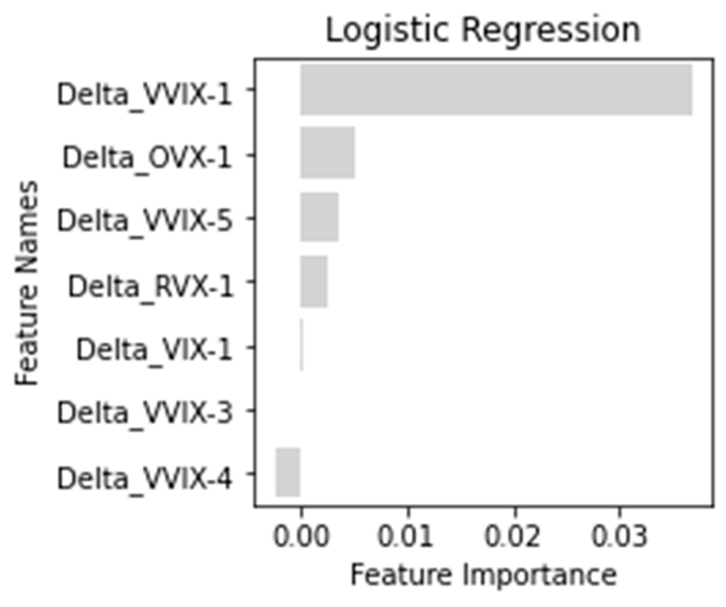
Logistic Regression: The logistic regression model achieved an accuracy score of 56.47% and an ROC AUC score of 56.71%. Its l1_ratio (L₁ and L₂ mixing parameter), as seen in Table 3, was 0.95. Due to a higher l1_ratio, which was indicative of more L₁ regularisation, most of the coefficient of redundant feature variables were set to zero and only seven were set to non-zero, which are stated in Table 8. Since these were coefficients, their absolute values were compared. According to Table 8, the coefficient of Delta_VVIX-1 was the most significant. Hence, it can be said that change in volatility of the CBOE VIX Index on the previous day is one of the most influential factors in predicting the present day’s binary movements of the India VIX Index. The top seven influencing factors, from highest to lowest in order, were Delta_VVIX-1, Delta_OVX-1, Delta_VVIX-5, Delta_RVX-1, Delta_VVIX-4, Delta_VIX-1 and Delta_VVIX-3. This clearly indicated that most of the US implied volatility indices had the predictive power in forecasting the India VIX Index. Most importantly, 1-day, 3-day, 4-day and 5-day prior changes in the volatility of the CBOE VIX Index (VVIX) were accountable, but the India VIX’s previous values did not count as an influencing factor.

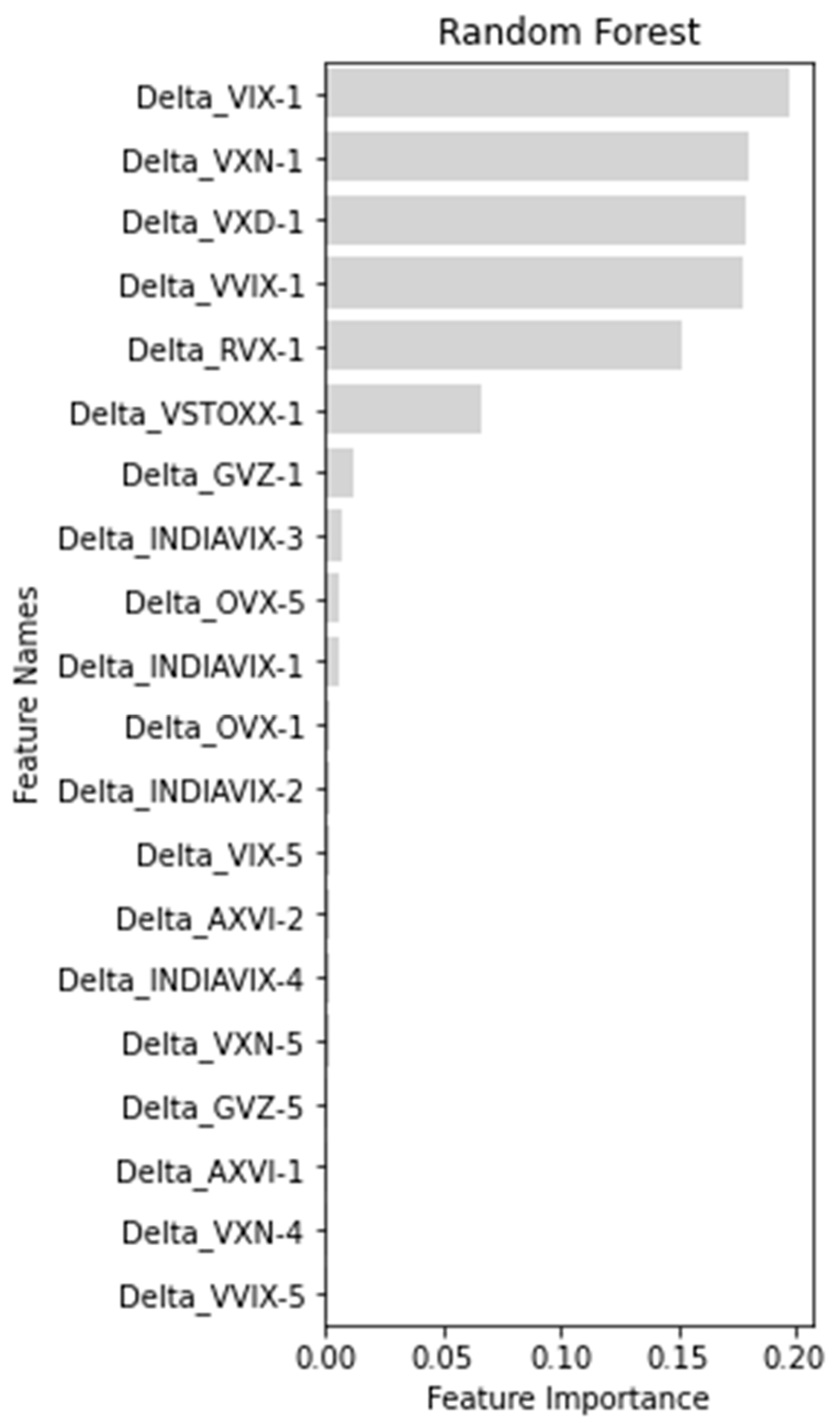
Random Forest: The Random Forest model achieved an accuracy score of 51.76% and an ROC AUC score of 55.49%. Table 7 and Figure 2 display the ranked feature variables from most to least important. There were only 20 feature variables set to non-zero; the rest were set to 0. From the top five ranked features, Delta_VIX-1, Delta_VXN-1, Delta_VXD-1, Delta_VVIX-1 and Delta_RVX-1 were the most significant, because their scores were significantly higher. These were the 1-day prior to changes in the US implied volatility indices, which affected the binary movement in the India VIX the most. As Delta_VSTOXX-1 was ranked 6th, the 1-day prior to changes in the Eurozone implied volatility index was also important. However, changes in the India VIX, as feature variables, were ranked 8th, 10th, 12th and 15th, among the top 20. Hence, changes in India VIX were not so important, but changes in the US implied volatility indices were most important in predicting the India VIX Index.

XG Boost: The XG Boost model achieved an accuracy score of 60% and an ROC AUC score of 60.98%. It is evident from Table 9 that the top five features, Delta_VXN-1, Delta_VVIX-1, Delta_VXD-1, Delta_VIX-1 and Delta_RVX-1, were most significant because their scores were significantly higher. Additionally, they were all US implied volatility indices. Hence, a change in US implied volatility indices had a greater impact than other implied volatility indices on the binary movements of the India VIX Index. Unfortunately, among the top 20 features ranked in Table 9, changes in India VIX ranked 10th, 11th, 13th and 14th in predicting its own movements. The 1-day and 5-day prior changes in the Eurozone implied volatility index placed 6th and 7th. From Table 10, the 1-day prior changes in the Australian implied volatility index (AXVI), the 4-day prior Hang Seng implied volatility Index (VHSI), and the 5-day prior Japan implied volatility index (JNIV) ranked 23rd 27th and 32nd, respectively.

Considering the importance of feature variables decided by all three models, the previous day’s closing value of the US implied volatility indices, except for the CBOE Eurocurrency Volatility Index, were the most influential factors in predicting the present day’s binary movement of the India VIX Index. The Eurozone implied volatility index and India VIX were roughly placed thereafter. AXVI, VHSI and JNIV ranked after the US, Eurozone and India implied volatility indices. The findings revealed that the XG Boost performed best, compared to random forest and the most trusted traditional logistic regression, when finding the role of the global volatility indices in forecasting the volatility index of the Indian economy.

5. Conclusions

To achieve the stated goal, logistic regression, Random Forest and XG Boost classifiers were applied on feature variables derived from changes in implied volatility indices across the globe, including the India VIX, and the target derived from the day-to-day upward and downward trend of the India VIX. XG Boost (Wang and Ni 2019) and Random Forest (Sadorsky 2021) were considered in this study because, like stock forecasting, volatility furcating is a time series forecasting, where variables exhibit temporal dependency and the relationship between target and features is likely to be nonlinear. Additionally, it provides a ranking for the complete list of features fed into the model, rather than eliminating redundant features, as is shown in Table 10. For a varied level of results, logistic regression and Random Forest were also considered. Logistic regression (Aliyeva 2021, August; Cheng et al. 2006; Zhang et al. 2022) was applied because its working mechanism is easily interpreted in eliminating redundant features without sacrificing accuracy. The fitted algorithms provided ranked feature variables that were fed into the models, and, following this, the models predicted binary labels for the testing datasets.

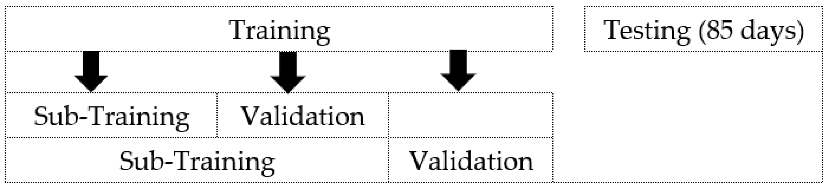
To analyse their significance, changes in the global implied volatility indices, including the India VIX, were taken as predictor variables, and binary labels, as the target variables, were created from changes in the closing value of the India VIX. Then, logistic regression, Random Forest and XG Boost were utilised on the data sample prepared from 18 September 2009, to 2 December 2021, to rank the feature variables. After performing 2-fold time series cross-validation, the ranked feature variables were captured, and the models predicted for the testing dataset.

It was evident from the results that the previous day’s changes in closing value of the US implied volatility indices, except for the CBOE Eurocurrency Volatility Index, were the most influential factors in predicting the present day’s binary movements of the India VIX. The Eurozone implied volatility index and the India VIX were placed thereafter. AXVI, VHSI and JNIV ranked after the US, Eurozone and Indian implied volatility indices.

It can be concluded that the India VIX was impacted most by the previous day’s changes in the closing value of the US implied volatility indices, except for the Chicago Board Options Exchange (CBOE) Eurocurrency volatility index. Additionally, the Eurozone implied volatility index was also important. However, the implied volatility indices of Australian Hang Seng and Japan were the least important.

Implication: It is important for traders and investors of emerging economies, like India’s economy, to know the influencing power of various global implied volatility indices in predicting the movement of the volatility index of the emerging economy, which, in turn, estimates the risk in that economy’s stock market. The outcome of this research is crucial for traders and investors of Indian economies in estimating risk in the stock market by creating a watch list of the most crucial global implied volatility indices. Hedgers, risk-averse investors, portfolio managers, and options and volatility traders are more interested in minimising risk over maximising return and the predicted value of the VIX Index could be very useful to them.

Contribution: Generally, to analyse the significance of independent variables (features), a regression technique is used, while considering features and target variables in the same timeline, and, subsequently, hypothesis testing is performed. However, this study considered a different approach to investigate the significance of feature variables for forecasting volatility, while considering features and target variables in a different timeline. Hence, this study provides another technique for significance testing.

Limitation and future scope: This study is restricted to the India VIX Index, but similar implied volatility indices of other emerging economies could be investigated in the future. In addition to the Random Forest and XG Boost, other ensemble learning algorithms, required to rank the set of feature variables, could be used in future studies.