Article

mSHAP: SHAP Values for Two-Part Models

1
Department of Statistics, Donald Bren School of Information and Computer Science, University of California-Irvine, Irvine, CA 92697, USA
2
Department of Statistics, College of Physical and Mathematical Sciences, Brigham Young University, Provo, UT 84602, USA
*
Author to whom correspondence should be addressed.
Submission received: 27 October 2021 / Revised: 13 December 2021 / Accepted: 17 December 2021 / Published: 24 December 2021

Abstract

:
Two-part models are important to and used throughout insurance and actuarial science. Since insurance is required for registering a car, obtaining a mortgage, and participating in certain businesses, it is especially important that the models that price insurance policies are fair and non-discriminatory. Black box models can make it very difficult to know which covariates are influencing the results, resulting in model risk and bias. SHAP (SHapley Additive exPlanations) values enable interpretation of various black box models, but little progress has been made in two-part models. In this paper, we propose mSHAP (or multiplicative SHAP), a method for computing SHAP values of two-part models using the SHAP values of the individual models. This method will allow for the predictions of two-part models to be explained at an individual observation level. After developing mSHAP, we perform an in-depth simulation study. Although the kernelSHAP algorithm is also capable of computing approximate SHAP values for a two-part model, a comparison with our method demonstrates that mSHAP is exponentially faster. Ultimately, we apply mSHAP to a two-part ratemaking model for personal auto property damage insurance coverage. Additionally, an R package (mshap) is available to easily implement the method in a wide variety of applications.

1. Introduction

One of the most popular families of machine learning models are tree-based algorithms, which use the concept of many decision trees working together to create more generalized predictions (Lundberg et al. 2020). Current implementations include random forests, gradient boosted forests, and others. These models are very good at learning relationships and have proven highly accurate in diverse areas. Currently, many aspects of life are affected by these algorithms as they have been implemented in business, technology, and more.
As these methods become more abundant, it is crucial that explanations of model output are easily available. Although there have been some advances in quantifying the uncertainty around black-box predictions as in Ablad et al. (2021), we search for more interpretable explanations that relate inputs to model outputs. The exact definition of “explanation” is a subject of debate, and Lipton (2018) argues that the word is often used in a very unscientific manner due to the confusion over its meaning. In this paper, we will regard an explainable system as what Doran et al. (2017) refer to as a comprehensible system, or one that “allow[s] the user to relate properties of the inputs to their output”.
Explainable models are important not only because some industries require them but also because understanding the why behind the output is essential to avoiding possible pitfalls. Understanding the reasoning behind model output allows for recognition of model bias, and increased security against the risk of harmful models being put into production. When implemented well, machine learning models can be more accurate than compared to traditional models. However, more accurate model families can be less explainable simply because of the nature of these algorithms. Generally, as predictive performance increases, model complexity also increases, decreasing the ability to understand the effects of inputs on the output (Gunning 2017).
In this paper, we propose a methodology for explaining two-part models, which expands on the already prevalent TreeSHAP (Tree Model SHapley Additive exPlanations) algorithm (Lundberg et al. 2020). This methodology, called mSHAP, will allow the output of two models to be multiplied together while maintaining explainability of the resulting prediction and deals with the issue of perturbation as described in (Li et al. 2020). Although there have been significant advancements made in this area, current methods are unable to rapidly assign input contributions to outputs in two-part models. This lack of explainability is an issue in the insurance industry, and here we propose a method of explaining two-part models that works rapidly and effectively.
The remainder of the paper is outlined as follows. In Section 2, we revisit existing SHAP-based methods and discuss where issues arise in the context of two-part models. In Section 3, we discuss the math behind multiplying SHAP values and propose a context in which SHAP values for two existing models can be combined to explain a two-part model. Although this framework is robust, it does leave a part (which we call α ) of the ultimate prediction that must be distributed back into the contributions of the variables. To this end, we run a simulation in Section 4 across different methods of distributing α and score the methods in comparison to kernelSHAP, which is an existing method for estimating explanations of any type of model. Having scored these methods, we select the best one and apply the process of mSHAP on an auto insurance dataset in Section 5. A conclusion and summary of our results is provided in Section 6.

2. Motivation

The initial idea for this methodology came due to the problem of machine learning in auto insurance ratemaking (or pricing). Actuaries are tasked with taking historical data and using it to set current rates for insured consumers. Given the sensitive nature of the data and the potential impact it has to bias rates for different types of people, there are strict regulations on the models. The outputs of these models must be explainable so that regulators in the insurance industry can be sure that the rates are not unfairly discriminatory.
Many actuaries use a two-part model to set rates, where the first part predicts how many claims a policyholder will have (the claim frequency) and the second part predicts the average cost of an individual claim (Frees and Sun 2010; Heras et al. 2018; Prabowo et al. 2019). Multiplying the two outputs of these models predicts the total cost of a given policyholder.
Two-part models are more difficult to explain than compared standard models, but the complexity increases when the two models themselves are not traditionally generalized linear models. Given this difficulty and the strict requirements of the regulators, machine learning models are not often used in actuarial ratemaking. Despite the lack of current industry use, machine learning models such as tree-based algorithms could improve the accuracy of ratemaking models (Akinyemi and Leiser 2020). Since the data that actuaries work with is typically tabular, tree-based algorithms are a good fit for predicting on the data. In recent years, there have been many advances in explaining tree-based machine learning algorithms, which could result in greater adaptation in the field. One of the most important is the SHAP value.

2.1. SHAP Values and Current Implementations

SHAP values originate in the field of economics, where they are used to explain player contributions in cooperative game theory. Proposed by Shapley (1953), they predict what each player brings to a game. This idea was ported into the world of machine learning by Lundberg and Lee (2017). The basic algorithm calculates the contribution of a variable to the prediction for every possible ordering of variables, then it averages those contributions. This becomes computationally impractical very quickly, but Lundberg and Lee (2017) created a modified algorithm that approximates these SHAP values.
A couple of years later, Lundberg et al. (2020) published a new paper detailing a method called TreeSHAP. This method is a rapid method for computing exact SHAP values for any tree-based machine learning model. The fixed structure of trees in a tree-based model allows shortcuts to be taken in the computation of SHAP values, which greatly speeds up the process. With this improvement, it becomes feasible to explain millions of predictions from tree-based machine learning algorithms. These local explanations can then be combined to create an understanding of the entire model.

2.2. Properties of SHAP Values

There are three essential properties of SHAP values: local accuracy/efficiency, consistency/monotonicity, and missingness (Lundberg and Lee 2017). These three properties are satisfied by the equation used to calculate SHAP values, as implemented by Lundberg and Lee (2017). While we focus on the local accuracy property for the rest of this section, we note that since mSHAP is built on top of treeSHAP, it automatically incorporates consistency/monotonicity and missingness properties.

2.2.1. Local Accuracy in Implementation

The most important of the above mentioned properties in the context of mSHAP is the property of local accuracy/efficiency. In the context of machine learning, this property says that the contributions of the variables should add up to the difference between the prediction and the average prediction of the model. The average prediction can be thought of as the model bias term, which is what the model will predict, on average, across all inputs (assuming representative training data). For a more mathematical definition of local accuracy, see Appendix A. In the TreeSHAP algorithm, the average prediction of the model is computed as the mean of all predictions for the training data set. The SHAP values are then computed to explain deviance from the average prediction.
Thus, given an arbitrary model Y with prediction y ^ based on two predictors, x 1 and x 2 , we can represent the mean prediction with μ Y and the SHAP values for the two covariates as s x 1 and s x 2 . Based on the property of local accuracy, we know that y ^ = μ Y + s x 1 + s x 2 .
This principle applies to models with any number of predictors and is very desireable in explainable machine learning (Arrieta et al. 2020).

2.2.2. The Problem of Local Accuracy

Since it is so important that the SHAP values add up to the model output, any attempt at explaining two-part model output from the SHAP values of the individual parts must maintain this property. However, multiplying the output of two models blends the contributions from different variables, making it unclear what contributions should be given to what variables. The idea of combining models and using SHAP values of the individual models to obtain the SHAP values for the combined model has been implemented before. In a related github issue, Scott Lundberg assures that averaging model output is compatible with averaging SHAP values, as long as the SHAP values (and model output) are in their untransformed state (Slundberg 2020). Even though averaging SHAP values for each variable works when averaging model outputs, the same principle does not apply when multiplying model outputs.
When considered, this is apparent. In the most simple of cases, we observe that if we have two models that both predict some outcomes based on two covariates x 1 and x 2 , we can average their results and likely obtain a better prediction. We will call these models A and B, respectively. For a given observation, model A predicts a ^ and model B predicts b ^ . When run through a SHAP explainer, we can break down these predictions even further. Since SHAP values are additive, we know that a ^ = μ A + s x 1 a + s x 2 a and b ^ = μ B + s x 1 b + s x 2 b . It follows the following is obtained.
avg ( a ^ , b ^ ) = a ^ + b ^ 2 = μ A + s x 1 a + s x 2 a + μ B + s x 1 b + s x 2 b 2 = μ A + μ B 2 + s x 1 a + s x 1 b 2 + s x 2 a + s x 2 b 2 = avg ( μ A , μ B ) + avg ( s x 1 a , s x 1 b ) + avg ( s x 2 a , s x 2 b ) .
Equation (1) means that we can find the contribution to the overall model from x 1 by averaging s x 1 a and s x 1 b , and likewise for the contribution to the overall model from x 2 .
However, if we for some reason wished to stack our models such that the two outputs ( a ^ and b ^ ) are multiplied, we run into a problem. This occurs because, despite the longings of all algebra students, the following is the case.
a ^ b ^ = ( μ A + s x 1 a + s x 2 a ) ( μ B + s x 1 b + s x 2 b ) μ A μ B + s x 1 a s x 1 b + s x 2 a s x 2 b .
Instead, we end up with the following.
a ^ b ^ = ( μ A + s x 1 a + s x 2 a ) ( μ B + s x 1 b + s x 2 b ) = μ A μ B + μ A s x 1 b + μ A s x 2 b + s x 1 a μ B + s x 1 a s x 1 b + s x 1 a s x 2 b + s x 2 a μ B + s x 2 a s x 1 b + s x 2 a s x 2 b .
Even in this simple case, it is difficult to assign a single contribution to our two different variables when presented with the SHAP values of the two original models. This problem grows even more difficult with the addition of other explanatory features. mSHAP is the methodology developed to solve this problem.

3. The Math behind Multiplying SHAP Values

In a two-part model, the output of one model is multiplied by the output of a second model to obtain the response. The principal driver behind mSHAP is the explanation of these sorts of models, and it requires that the SHAP values be multiplied together in some manner to obtain a final SHAP value for the output. The mathematics behind mSHAP are explained here in the general case for any given number of predictors with a training set of arbitrary size. Although an exact solution for the SHAP values of a two-part model is still out of reach, this method proves very accurate in its results.

3.1. Definitions

Consider three different predictive models, f , g , and h and a single input (training) matrix A. We will let the number of columns and rows in A be arbitrary. In other words, let A be an n × p matrix where each column is a covariate and each row is an observation. Moreover, let A i denote the ith observation (row) of A. Furthermore, define h to be the product of f and g; thus, h ( A i ) = f ( A i ) · g ( A i ) .
Recall that the sum of the SHAP values for each covariate and the average model output must add up to the model prediction. For simplicity in presentation, we will define f ( A i ) = x i ^ , g ( A i ) = y i ^ , and h ( A i ) = z i ^ and the contribution of the jth predictor to x i as s x i j . With these considerations in place, we can define the output space of our three models on the training data set, as shown in Equations (3) to (5).
For model f, we have the following.
x 1 ^ = s x 1 1 + s x 1 2 + s x 1 3 + + s x 1 p + μ f x 2 ^ = s x 2 1 + s x 2 2 + s x 2 3 + + s x 2 p + μ f x 3 ^ = s x 3 1 + s x 3 2 + s x 3 3 + + s x 3 p + μ f x n ^ = s x n 1 + s x n 2 + s x n 3 + + s x n p + μ f
For model g, we have the following.
y 1 ^ = s y 1 1 + s y 1 2 + s y 1 3 + + s y 1 p + μ g y 2 ^ = s y 2 1 + s y 2 2 + s y 2 3 + + s y 2 p + μ g y 3 ^ = s y 3 1 + s y 3 2 + s y 3 3 + + s y 3 p + μ g y n ^ = s y n 1 + s y n 2 + s y n 3 + + s y n p + μ g
Moreover, for model h, we have the following.
z 1 ^ = s z 1 1 + s z 1 2 + s z 1 3 + + s z 1 p + μ h z 2 ^ = s z 2 1 + s z 2 2 + s z 2 3 + + s z 2 p + μ h z 3 ^ = s z 3 1 + s z 3 2 + s z 3 3 + + s z 3 p + μ h z n ^ = s z n 1 + s z n 2 + s z n 3 + + s z n p + μ h
Furthermore, given our training data A, we can extract the values of μ f , μ g , and μ h . As explained above, these are the average values of the model predictions on the training set.
μ f = 1 n i = 1 n x i ^ = x 1 ^ + x 2 ^ + x 3 ^ + + x n ^ n
μ g = 1 n i = 1 n y i ^ = y 1 ^ + y 2 ^ + y 3 ^ + + y n ^ n
μ h = 1 n i = 1 n z i ^ = z 1 ^ + z 2 ^ + z 3 ^ + + z n ^ n
In practice, it is necessary to be able to pull μ h out of x i ^ y i ^ . When implemented, it is important to note that μ f μ g = μ f μ g μ h + μ h . Since every expansion of SHAP values from x i ^ x j ^ contains μ f μ g , we substitute μ f μ g μ h + μ h , where μ h is essential and μ f μ g μ h becomes a term that we label α and distribute among all the SHAP values. A more formalized definition of α is provide in Appendix B.

3.2. Obtaining z i ’s SHAP Values

We now derive the individual SHAP values for each variable as it pertains to the prediction of model h. Again, we will allow this output be an arbitrary z i ^ . Recall the following.
z i ^ = x i ^ y i ^ = ( s x i 1 + s x i 2 + s x i 3 + + s x i p + μ f ) ( s y i 1 + s y i 2 + s y i 3 + + s y i p + μ g ) .
Using a tabular form for visual simplicity, we obtain the following expansion of Equation (9).
s x i 1 + s x i 2 + s x i 3 + + s x i p + μ f s y i 1 s x i 1 s y i 1 s x i 2 s y i 1 s x i 3 s y i 1 s x i p s y i 1 μ f s y i 1 + s y i 2 s x i 1 s y i 2 s x i 2 s y i 2 s x i 3 s y i 2 s x i p s y i 2 μ f s y i 2 + s y i 3 s x i 1 s y i 3 s x i 2 s y i 3 s x i 3 s y i 3 s x i p s y i 3 μ f s y i 3 + + s y i n s x i 1 s y i p s x i 2 s y i p s x i 3 s y i p s x i p s y i p μ f s y i p + μ g s x i 1 μ g s x i 2 μ g s x i 3 μ g s x i p μ g μ f μ g
We break these terms into the SHAP values for each variable, one through p, for z i ^ . Our approach breaks s z i j into two parts, which we call s z i j and α i j . By using the method of obtaining α i , which can take on several forms, s z i j is always as follows (where j refers to the jth covariate).
s z i j = μ f s y i j + s x i j μ g + s x i j s y i j + a = 1 p ( s x i j s y i a 2 I ( a j ) ) + a = 1 p ( s y i j s x i a 2 I ( a j ) ) = μ f s y i j + s x i j μ g + 1 2 a = 1 p ( s x i j s y i a + s y i j s x i a )
In other words and with the aid of the table above, Equation (10) can be described as the sum of the jth row and jth column, where every term is divided by two except the terms with μ f and μ g . When applied to each variable, this can be written as follows:
z i ^ = j = 1 p μ f s y i j + s x i j μ g + 1 2 a = 1 p ( s x i j s y i a + s y i j s x i a ) + μ f μ g
and by applying the breakdown we derived in Equation (10), while simplifying Equation (11) as well, we arrive at the following.
z i ^ = j = 1 p s z i j + α + μ h .
For a proof that this formula and the subsequent distribution of α maintains the local accuracy property of SHAP values, refer to Appendix B.1.

3.3. Methods for Distributing α

We now arrive at the aforementioned point of deciding how to distribute α into each s z i j . There are four methods that we tested for distributing α : the first being simple uniform distribution and the others being variations of weighting based on the value of s z i j . All four of these methods maintain the local accuracy property of SHAP values, and a detailed proof of the absolute value case can be found in Appendix B.1. We acknowledge that there is no easy interpretation of α and our choices for distributing/weighting it were arbitrary methods of dividing a whole into parts. In Equation (13), we evenly distributed α over the contributions from all covariates, while in Equation (15), we weighted each part by its corresponding contribution to the model. Both Equations (16) and (17) are variations on weighting the parts, but they use different methods to ensure that all the weights are positive. Different methods for distributing α may be a topic for further research.

3.3.1. Uniformly Distributed

The simplest method of distributing α between all the s z i j ’s is to divide it evenly. In this case, our resulting equation for each variable’s SHAP value would be the following.
s z i j = s z i j + α p .
This method could prove a strong baseline.

3.3.2. Raw Weights

The computation of this method is made easier by recalling from Equation (11) that the following is the case:
j = 1 p s z i j = z i ^ μ f μ g ,
which allows us to use z i ^ μ f μ g as the whole upon which we base our weighting. When applied, this method defines each SHAP value as follows.
s z i j = s z i j + s z i j z i ^ μ f μ g α .

3.3.3. Absolute Weights

This method differs from that of the raw weights in that instead of summing the s z i j ’s, we sum their absolute values. The weight for each SHAP value is calculated with the following.
s z i j = s z i j + | s z i j | k = 1 p | s z i k | α .

3.3.4. Squared Weights

Finally, instead of working with the absolute values, we could work with squares. Similarly to the equation above, the SHAP values under this method are computed by the following.
s z i j = s z i j + ( s z i j ) 2 k = 1 p ( s z i k ) 2 α .

4. Simulation Study for Distributing α

To test the differences between these methods of distributing α , we simulated various multiplicative models based on known equations and compared the results of our multiplicative method with the output from kernelSHAP. KernelSHAP is an existing generalized method for estimating the contributions based on any prediction function. However, it is extremely computationally expensive when compared with TreeSHAP. When training on millions of rows with many variables, it becomes unrealistic to use kernelSHAP for computing the SHAP values.

4.1. Scoring the Methods

Several factors were considered in scoring, including the mean absolute error of the SHAP values, the directions of the SHAP values, and the rank (in magnitude) of the SHAP values for each variable. The score needed to be a singular method to asses how close the method approaches the kernelSHAP estimates. Even though kernelSHAP is an estimate and not necessarily the truth, we used it as a benchmark in the different parts of our score. This allowed us to compare new variations of the mSHAP method to existing methods for the computation of SHAP values.
For ease of notation, if we define the SHAP value, we are estimating it as s z i j ; then, we can define its counterpart as computed by kernelSHAP, as k z i j .

4.1.1. General Equation for Scoring

In the end, an equation was formed to create a raw “score” based on the direction of the SHAP value, the relative value of the SHAP value, and the rank (importance) of the SHAP value in comparison to kernelSHAP. The score ranges from 0 to 3 (with 3 being the best possible score), and is defined by the following:
β ( s z i j , k z i j | θ 1 , θ 2 ) = λ 1 ( s z i j , k z i j | θ 1 ) + λ 2 ( s z i j , k z i j | θ 2 ) + λ 3 ( s z i j , k z i j )
where the following is the case:
λ 1 ( s z i j , k z i j | θ 1 ) = 1 s z i j k z i j > 0 min ( 1 , 1 + θ 1 | s z i j | + | k z i j | + θ 1 ) otherwise
λ 2 ( s z i j , k z i j | θ 2 ) = min ( 1 , 1 + θ 2 | s z i j k z i j | + 1 )
λ 3 ( s z i j , k z i j ) = 1 | imp ( s z i j ) imp ( k z i j ) | + 1
and imp ( s z i j ) is the importance of that SHAP value relative to the other contributions in the observation (where importance is determined by the magnitude of the absolute value).
In this function (and as will be described in the following section), λ 1 is the contribution from the signs of the SHAP values, λ 2 is the contribution from the relative value of the SHAP values, and λ 3 is the contribution from the relative ranking (importance) of the SHAP values.

4.1.2. Lambda Functions

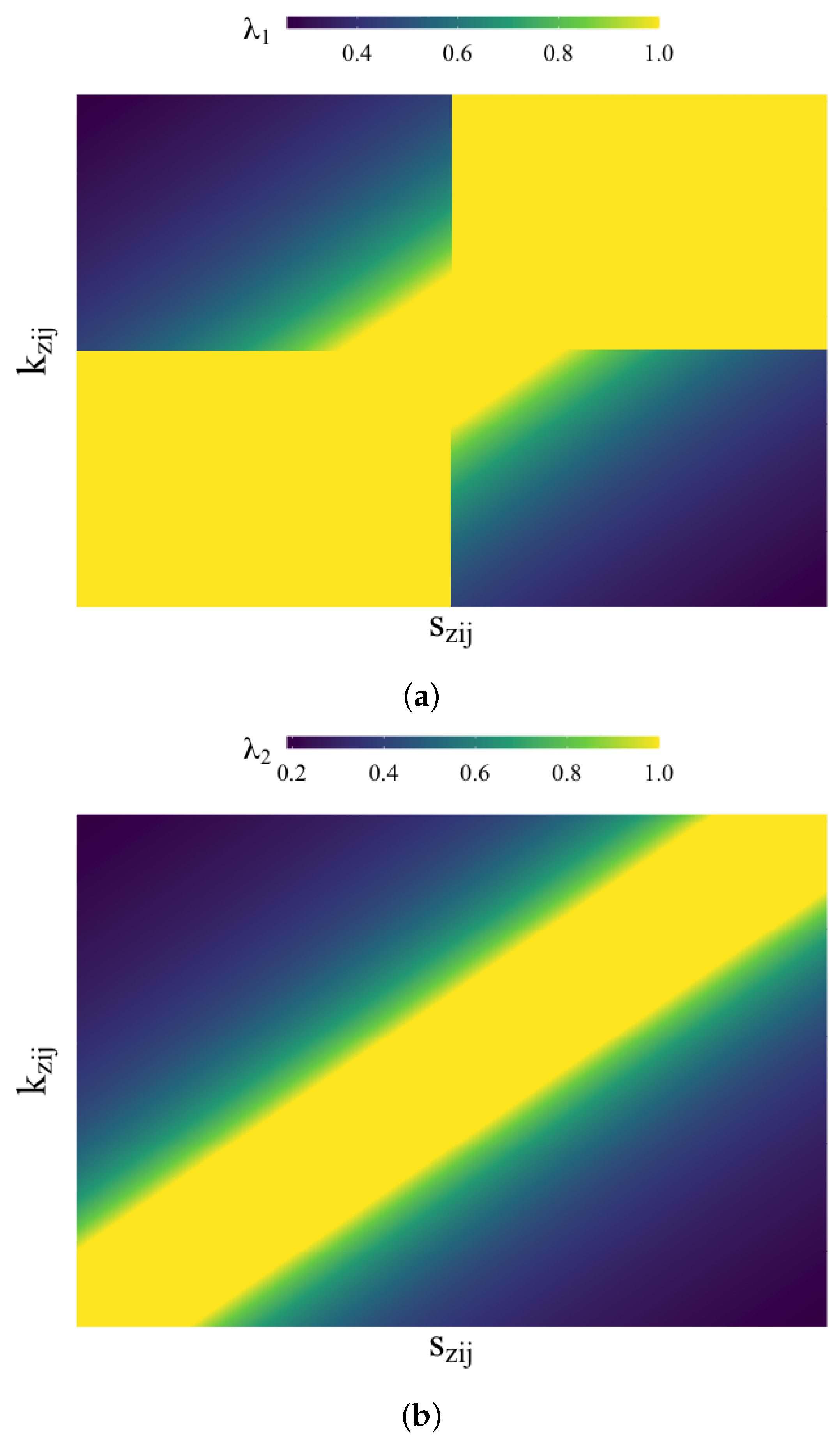
In order to gain some intuition about the λ functions (Equations (19)–(21)) and the impact of θ 1 and θ 2 , we depict them in Figure 1.
For λ 1 , which measures whether the two SHAP values are the same sign, any values in the first and third quadrants return a perfect score of 1, since the two values have the same sign. It also allows for some wiggle room with θ 1 by allowing anything within the lines k z i j = s z i j + θ 1 and k z i j = s z i j θ 1 to be 1. Beyond those boundaries, the scores gradually decrease.
The function λ 2 , which compares the values, also creates boundary lines for the perfect score of 1 at k z i j = s z i j + θ 2 and k z i j = s z i j θ 2 . In other words, as long as the difference between s z i j and k z i j is less than θ 2 , the function will return 1. Beyond that, the value begins to decrease.
Out of the three λ 3 , the rank measure is the easiest to understand. In a given observation, each SHAP value is given a rank (between 1 and p, inclusive) based on its absolute value. These ranks are then compared, and the closer they are together, the higher the score, with a perfect score of 1 being obtained if the two rankings are the same.

4.2. Simulation Study

As mentioned above, we simulated various multiplicative models based on known equations and compared the results of our multiplicative method with the output from kernelSHAP in order to test the model. The type of simulation used here is a Monte Carlo simulation that is commonly used in actuarial literature, as in Appendix C Romaniuk (2017).
Specifically, we used three variables, x 1 , x 2 , and x 3 in a variety of response equations y 1 and y 2 to create models for y 1 and y 2 and then multiply their outputs together. Using the multiplied output and the covariates, we were able to use kernelSHAP to compute an estimate of the SHAP values. We could then compared this estimate to the result from our multiplicative method, as described above, with different methods of distributing α applied.
More details on the simulation can be found in Appendix C.
For testing, we used 100 samples in each iteration for faster computation, which allowed us to simulate over 2500 scenarios. Specifically, we worked with all possible combinations of the following values (see Table 1).
For each combination of values in the above table, we distributed α in each of the four methods mentioned in Section 3.3. The resulting table, therefore, had results for each model and each method of distributing α . In general, we averaged across all rows of the same method to obtain the scores that were compared to each other.
In our examples, our covariates were distributed as follows.
x 1 Uniform [ 10 , 10 ] x 2 Uniform [ 0 , 20 ] x 3 Uniform [ 5 , 1 ] .

4.3. Results of the Simulation

In general, the multiplicative SHAP method performed very well when compared to the kernelSHAP output. Since kernelSHAP is an estimation as well, it is hard to determine exactly how well the multiplicative SHAP method does, but we will summarize some statistics here.

4.3.1. Distributing α

After trying the aforementioned four methods for distributing α into the SHAP values, we came to the conclusion that the weighted by absolute value method was the best. This came by way of the score as well as other metrics. Details can be observed in the Table 2 (all values are averaged across all 2520 simulations).

4.3.2. Impact of θ 1 and θ 2

We plotted the effects of the different values for θ 1 and θ 2 on the overall score based on type of method of distribution.
As observed, in Figure 2 and Figure 3, changing the value of these two parameters has a similar impact across all scoring methods.

4.3.3. Computational Time

The most dramatic benefit of mSHAP over kernelSHAP is the computational efficiency of mSHAP. The times shown in this section were obtained using a personal MacBook Air laptop computer with a 1.8 GHz Dual-Core Intel Core i5 processor.
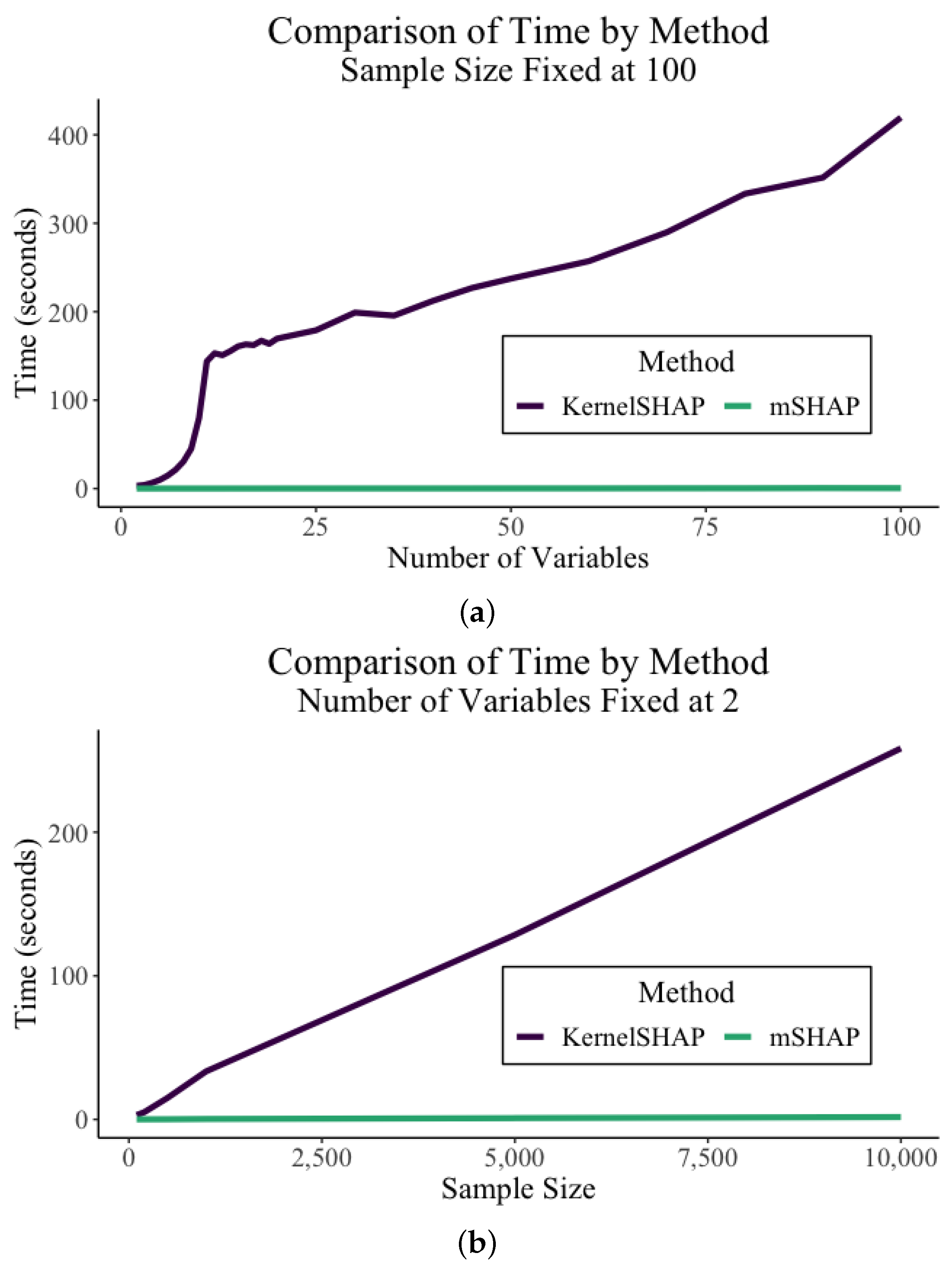
In Figure 4, we are able to observe the comparison in run time between the kernelSHAP and mSHAP methods (including the individual treeSHAP value calculations). Both an increase in the number of variables and the number of samples causes the time of kernelSHAP to grow greatly, while the multiplicative method remains fairly constant. In these trials, the number of background samples was fixed at 100 for kernelSHAP.
A case study can show the importance of this. In the auto insurance dataset, there are 5,000,000 rows in the test set, with 46 variables. For the sake of simplicity, let us assume that we use 45 of those variables and that 100 background samples are enough to compute accurate SHAP values. In reality, it would need many more background samples, but that only accentuates the point, as a large quantity of background samples slows kernelSHAP drastically. KernelSHAP computes SHAP values for 45 variables at a rate of about 2.268 s per observation on a personal laptop. In order to compute the SHAP values for the entire test set, one would need about 131 days of continuous compute time.
In contrast, our multiplicative method, using treeSHAP on two tree-based models, computes SHAP values at a rate of about 0.00175 s per observation for a model with 45 variables. To compute the SHAP values for the entire test set using this method, it would take a little less than three hours of continuous computation time.

4.4. Final Equation for mSHAP

Based on the results of the simulation, we determine that the best method of distributing α is the method of weighting by absolute values (as described above). Recall from Equation (16) that in this method, we have the following:
s z i j = s z i j + | s z i j | k = 1 p | s z i k | ( α )
and that s z i j refers to an initial mSHAP value, before the correction introduced by α as in Equation (10). It is calculated as follows.
s z i j = μ f s y i j + s x i j μ g + 1 2 a = 1 p ( s x i j s y i a + s y i j s x i a ) .
Thus, the final equation for the mSHAP value of the jth predictor on the ith observation can be written as follows.
s z i j = μ f s y i j + s x i j μ g + 1 2 a = 1 p ( s x i j s y i a + s y i j s x i a ) + | s z i j | k = 1 p | s z i k | ( α ) .
For a complete proof that local accuracy holds with this equation, see Appendix B.1.

5. Case Study

In order to prove the efficacy of mSHAP, it is necessary to put it into practice. We obtained an insurance dataset including over 20 million auto insurance policies for a large insurance provider in the United States. Using these data, we created a two-part model that predicts the expected property damage cost of each policy. Both parts of this model consist of tree-based methods, specifically random forests. After creating this model, we used the shap python library to explain the predictions of each individual part on a sample of 50,000 observations from our test set. We then applied the final mSHAP method, as described above, to obtain explanations for the overall model and used the mshap R package to visualize some of the results. Although there has been recent studies on models that span multiple types of claims on one policy as in Gómez-Déniz and Calderín-Ojeda (2021), the data were such that we could only focus on one specific type of claim for each model.

5.1. Model Creation

As mentioned above, the model is a two-part model for predicting the expected cost of the policy. The first part of the model predicts the frequency of the claims. It is a random forest that predicts the probability of each of four possible outcomes (a multinomial model). In our dataset, there existed policies with up to seven claims, but we chose the classes of zero, one, two, and three and bundled everything over three into the third class. The data were heavily imbalanced; thus, we used a combination of upsampling the minority classes (one, two, and three claims) and downsampling the majority class (0 claims) to obtain a more balanced training data set. This allowed the model to use the information to predict meaningful probabilities instead of always assigning a very high probability to zero claims.
The second part is a random forest which predicts the severity component of the two-part model or the expected cost per claim.
Once these models were created, we could calculate the expected value (or in this case, the expected cost) of a policy in the following manner. If we let P i ^ ( a ) denote the predicted probability of the for the ith policy of the ath class and y i ^ be the predicted severity of the policy, then we have the following.
E V = y i ^ 0 P i ^ ( 0 ) + 1 P i ^ ( 1 ) + 2 P i ^ ( 2 ) + 3 P i ^ ( 3 )
The final two-part model was used to predict the expected cost of 50,000 policies from the test dataset. For more specific details about the model and how it was tuned, see Appendix E.

5.2. Model Explanation

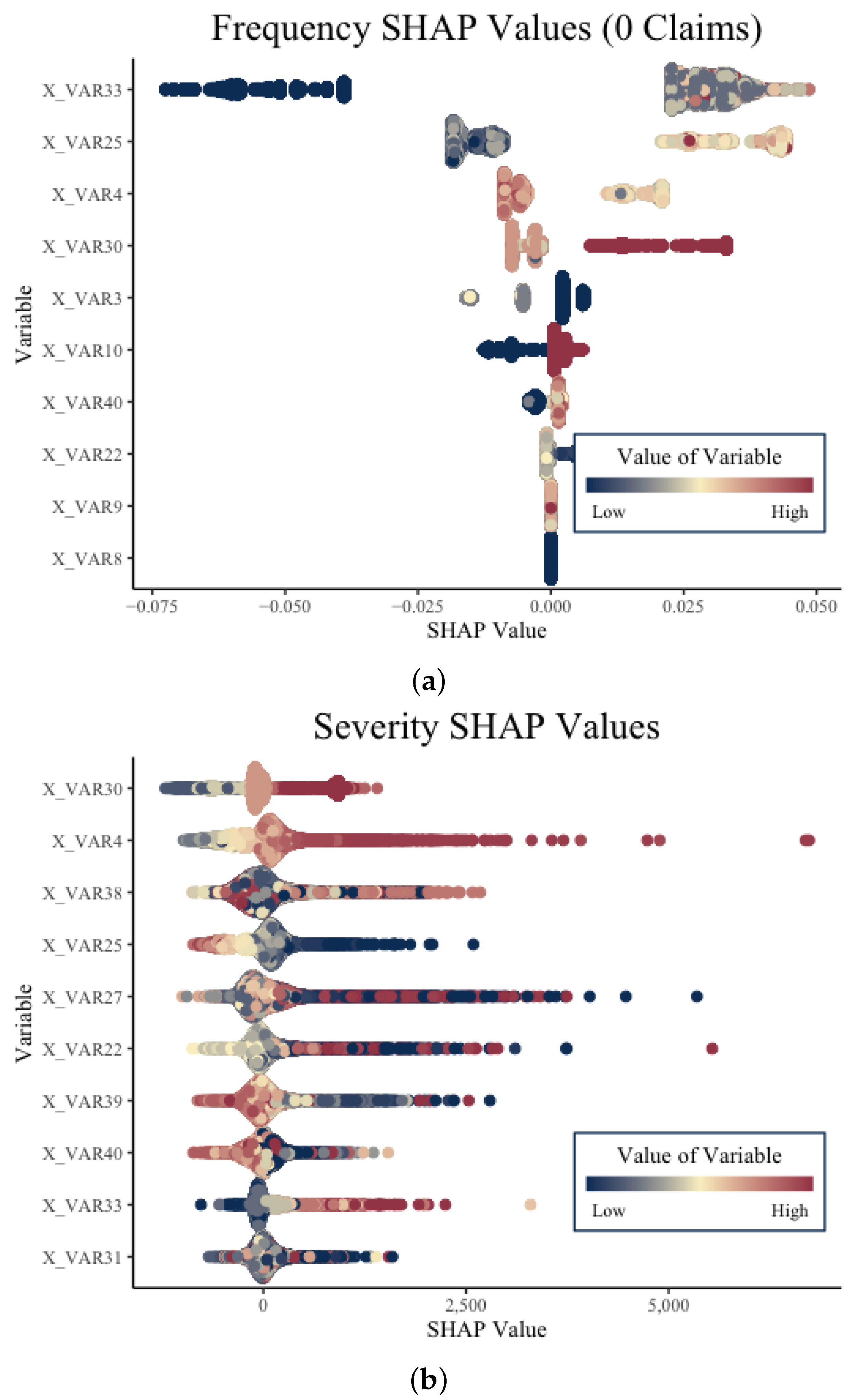
After creating the two-part model and obtaining final predictions for the expected cost of the claims, we were able to apply mSHAP to explain final model predictions. Before performing this, we computed SHAP values on the individual models so that we have the necessary data to apply the mSHAP method for explaining two-part models. Summary plots for the five different sets of SHAP values (one for severity, and one for each class of the frequency model) can be created. In Figure 5, we depict the SHAP values for one of the frequency classes from the frequency model and the SHAP values for the severity model.
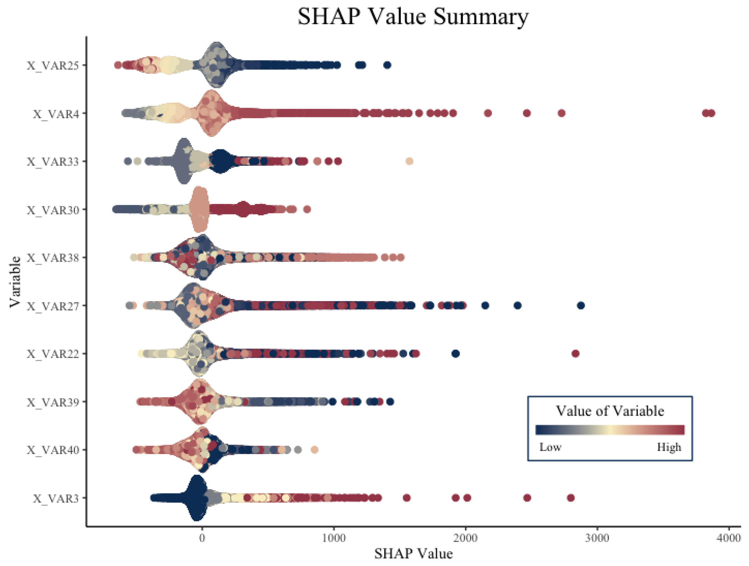
After computing these SHAP values, we applied the mSHAP method detailed in this paper. When applying mSHAP, the expected value formula above is simply a linear combination, and we are able to perform that same linear combination on the SHAP values before (or after) applying mSHAP. This process left us with a single mSHAP value for each variable in every row of our test set and an overall expected value across the training set. The summary plot of those final mSHAP values can be oberved in Figure 6, and an example of an observation plot is shown in Figure 7.
The beauty of the mSHAP method is that it allows for a two-part model to be explained in the same manner that tree-based models can be easily explained with SHAP values. As observed in the plots, general trends across variables can be established, as well as specific policies dissected to observe individual motivators behind each prediction. The ability of mSHAP to explain these types of models opens the door to using two-part models that are both powerful and explainable.
6. Conclusions

In this paper, we developed mSHAP, a method for calculating SHAP values in two-part models. The theoretical foundations were laid out, and the algorithm was explained. Our method is shown to be much less computationally expensive than kernelSHAP on the order of hundreds of times faster (See Section 4.3). Furthermore, the results of the application to a real-world problem are displayed. We recommend that this new algorithm be implemented in the insurance industry where two-part models are used heavily. It will allow for insurance pricing to be explained to key stakeholders while ensuring fair and accurate pricing methods with black-box algorithms. Although this new framework is robust and builds upon exact SHAP values of individual model parts, it does not return exact SHAP values for the two-part model. Further research is needed to develop exact methodologies for determining variable contributions in two-part models.

Author Contributions

Data curation, S.M.; formal analysis, B.H.; funding acquisition, B.H.; investigation, S.M.; methodology, S.M.; project administration, B.H.; writing—original draft, S.M.; writing—review and editing, B.H. All authors have read and agreed to the published version of the manuscript.

Funding

This paper was funded by an individual grant from the Casualty Actuarial Society.

Institutional Review Board Statement

Not applicable.

Informed Consent Statement

Not applicable.

Data Availability Statement

Data was provided by a private insurance carrier to the Casualty Actuarial Society (CAS) after anonymizing the data set. This data is available to actuarial researchers for well-defined research projects that have universal benefit to the insurance industry and the public. In order to obtain the data, contact CAS through Brian Fannin with a project proposal.

Acknowledgments

Brigham Young University Department of Statistics Computing Cluster; Brian Fanin and the Casualty Actuarial Society for providing the data; and Isabelle Matthews for proofreading.

Conflicts of Interest

The authors declare no conflict of interest.

Appendix A. Shapley Values

In this section, we briefly discuss the math behind Shapley values. This section leans heavily upon the explanations and formulas as given in Lundberg and Lee (2017). A motivated reader can find further information regarding Shapley values in that paper.
Shapley values are a class of what is known as additive feature attribution methods. These methods are defined as methods that have an “explanation model that is a linear function of binary variables”:
g ( z ) = ϕ 0 + i = 1 M ϕ i z i
where M is the number of input features, ϕ 0 , ϕ i R and z i { 0 , 1 } M . Essentially, every prediction of the model (which we will denote f ( x ) ) can be obtained by assigning some contribution to each of the variables.
The Shapley values have three desirable properties, as mentioned above, and the formal definitions for these properties are given here.
Local Accuracy. Local accuracy requires that the outputs of our model f ( x ) and the outputs of the additive feature attribution method to be equal. In symbols, this means the following.
f ( x ) = g ( x ) = ϕ 0 + i = 1 M ϕ i x i .
Missingness. A second property is missingness. Simply stated, any variable that has a value of 0 requires its corresponding contribution to the output to be zero. In other words, the following is the case.
x i = 0 ϕ i = 0
Consistency. The third property is consistency, which assures that if the model changes so that an input’s contribution increases or stays the same, the attribution of that input should not decrease. If we let f x ( z ) = f ( h x ( z ) ) and z / i denote setting z i = 0 , then for any two models f and f , if the following is the case:
f x ( z ) f x ( z / i ) f x ( z ) f x ( z / i )
for all inputs z { 0 , 1 } M , then ϕ i ( f , x ) ϕ i ( f , x ) .
The theorem proposed by Lundberg and Lee (2017) is as follows. Only one possible explanation model follows the above definition and the three given properties:
ϕ i ( f , x ) = z x | z | ! ( M | z | 1 ) ! M ! [ f x ( z ) f x ( z / i ) ]
where | z | is the number of non-zero entries in z and z x represents all z vectors where the non-zero entries are a subset of the non-zero entries in x .

Appendix B. The Relationship between μf, μg, and μh

Recall from Equation (8) that the following is the case:
μ h = 1 n i = 1 n z i ^ = z 1 ^ + z 2 ^ + z 3 ^ + + z n ^ n ,
and that we defined model h as the product of models f and g. Thus, any z i ^ is equivalent to x i ^ y i ^ .
Taking Equation (8) and substituting x i ^ y i ^ for every z i ^ , we see that the following is the case.
μ h = x 1 ^ y 1 ^ + x 2 ^ y 2 ^ + x 3 ^ y 3 ^ + + x n ^ y n ^ n .
Whenever we multiply x i ^ and y i ^ to obtain z i ^ , it is inevitable that we end up with the term μ f μ g in the resulting expansion. We will take this term and split it into two parts: μ h and α . Some correction must be added in to the other SHAP values. Start with the expansion of μ f μ g :
μ f μ g = ( 1 n i = 1 n x i ^ ) · ( 1 n i = 1 n y i ^ )
which can be written in tabular form for ease of explanation.
x 1 ^ n + x 2 ^ n + x 3 ^ n + + x n ^ n y 1 ^ n x 1 ^ y 1 ^ n 2 x 2 ^ y 1 ^ n 2 x 3 ^ y 1 ^ n 2 x n ^ y 1 ^ n 2 + y 2 ^ n x 1 ^ y 2 ^ n 2 x 2 ^ y 2 ^ n 2 x 3 ^ y 2 ^ n 2 x n ^ y 2 ^ n 2 + y 3 ^ n x 1 ^ y 3 ^ n 2 x 2 ^ y 3 ^ n 2 x 3 ^ y 3 ^ n 2 x n ^ y 3 ^ n 2 + + y n ^ n x 1 ^ y n ^ n 2 x 2 ^ y n ^ n 2 x 3 ^ y n ^ n 2 x n ^ y n ^ n 2
Along the diagonal are the terms that may be of interest to us, specifically the following.
i = 1 n x i ^ y i ^ n 2 = μ h n .
By multiplying both sides by n, we see that the following is the case.
n i = 1 n x i ^ y i ^ n 2 = μ h .
Since we already have one, we can simply add n 1 and subtract n 1 summands to obtain the desired μ h . This can be summarized as follows:
μ f μ g = i = 1 n j = 1 n ( x i ^ y j ^ n 2 I ( i j ) ) ( n 1 ) i = 1 n x i ^ y i ^ n 2 + i = 1 n x i ^ y i ^ n = i = 1 n j = 1 n ( x i ^ y j ^ n 2 I ( i j ) ) ( n 1 ) i = 1 n x i ^ y i ^ n 2 + μ h = α + μ h
where α = i = 1 n j = 1 n ( x i ^ y j ^ n 2 I ( i j ) ) ( n 1 ) i = 1 n x i ^ y i ^ n 2 = μ f μ g μ h . This becomes a critical element in our substitutions in later steps.

Appendix B.1. Proof of Local Accuracy

If we define z i ^ as the prediction of our model, h for the ith observation, μ h as the average model prediction across our training set, and s z i j as the contribution of the jth variable to the ith observation’s prediction, we can define local accuracy as follows.
z i ^ = μ h + j = 1 p s z i j .
In this section, we will prove that this equation holds for our chosen definition of s z i j .
Remember that based on our initial definition, z i ^ = x i ^ y i ^ , and recall from Equation (24) that the final equation for the mSHAP values is as follows.
s z i j = μ f s y i j + s x i j μ g + 1 2 a = 1 p ( s x i j s y i a + s y i j s x i a ) + | s z i j | k = 1 p | s z i k | α .
We see that the following is the case.
μ h + j = 1 p s z i j = μ h + j = 1 p μ f s y i j + s x i j μ g + 1 2 a = 1 p ( s x i j s y i a + s y i j s x i a ) + | s z i j | k = 1 p | s z i k | α = μ h + μ f s y i 1 + s x i 1 μ g + 1 2 a = 1 p ( s x i 1 s y i a + s y i 1 s x i a ) + | s z i 1 | k = 1 p | s z i k | α + + μ f s y i p + s x i p μ g + 1 2 a = 1 p ( s x i p s y i a + s y i p s x i a ) + | s z i p | k = 1 p | s z i k | α = μ h + k = 1 p | s z i k | k = 1 p | s z i k | α + j = 1 p μ f s y i j + s x i j μ g + 1 2 a = 1 p ( s x i j s y i a + s y i j s x i a ) = μ h + α + j = 1 p μ f s y i j + s x i j μ g + 1 2 a = 1 p ( s x i j s y i a + s y i j s x i a )
At this point, we recall the definition given in Section 3.1 that μ f μ g μ h = α . With a simple manipulation, we see that μ h + α = μ f μ g . Thus, the following is the case.
= μ f μ g + μ f s y i 1 + s x i 1 μ g + 1 2 a = 1 p ( s x i 1 s y i a + s y i 1 s x i a ) + + μ f s y i p + s x i p μ g + 1 2 a = 1 p ( s x i p s y i a + s y i p s x i a ) = μ f μ g + j = 1 p μ f s y i j + j = 1 p s x i j μ g + 1 2 j = 1 p a = 1 p ( s x i j s y i a + s y i j s x i a ) .
We can expand this further to give us the following.
= μ f μ g + j = 1 p μ f s y i j + j = 1 p s x i j μ g + 1 2 ( s x i 1 s y i 1 + s y i 1 s x i 1 + s x i 1 s y i 2 + s y i 1 s x i 2 + + s x i 1 s y i p + s y i 1 s x i p + s x i 2 s y i 1 + s y i 2 s x i 1 + s x i 2 s y i 2 + s y i 2 s x i 2 + + s x i 2 s y i p + s y i 2 s x i p + + + s x i p s y i 1 + s y i p s x i 1 + s x i p s y i 2 + s y i p s x i 2 + + s x i p s y i p + s y i p s x i p ) = μ f μ g + j = 1 p μ f s y i j + j = 1 p s x i j μ g + 1 2 ( 2 s x i 1 s y i 1 + 2 s x i 1 s y i 2 + 2 s x i 1 s y i 3 + + 2 s x i 1 s y i p + 2 s x i 2 s y i 1 + 2 s x i 2 s y i 2 + 2 s x i 2 s y i 3 + + 2 s x i 2 s y i p + + + 2 s x i p s y i 1 + 2 s x i p s y i 2 + 2 s x i p s y i 3 + + 2 s x i p s y i p = ( μ f + s x i 1 + s x i 2 + + s x i p ) ( μ g + s y i 1 + s y i 2 + + s y i p ) .
Since the original SHAP values have the local accuracy property, we know that the following is the case.
( μ f + s x i 1 + s x i 2 + + s x i p ) ( μ g + s y i 1 + s y i 2 + + s y i p ) = x i ^ y i ^
In turn, this is equal to z i ^ . We see that z i ^ = μ h + j = 1 p s z i j and that the local accuracy property holds for the implementation of mSHAP using the absolute value weighting method for α . Based on Equation (A15), we see that as long as the method for weighting α sums to 1 across all covariates, the property of local accuracy holds. All methods tested in this paper of weighting α maintain the local accuracy property, and a proof of that is similar to the one above but left as an exercise for the reader. Since the final equation for mSHAP only uses the absolute value method of weighting, we only prove local accuracy for Equation (24) here.

Appendix C. The Simulation

Appendix C.1. Simulation Process

The basic flow for the simulation involved creating a data frame with all our desired combinations of y 1 , y 1 , θ 1 , and θ 2 and then mapping by using the following steps for each row:
  • Using randomly distributed data as the covariates, create the response variables by evaluating y 1 and y 2 and then multiply them together;
  • Create two gradient boosted forests, one to predict y 1 and the other to predict y 2 , based on the covariates;
  • Multiply the model predictions together and run kernelSHAP to approximate explanations for the final model output;
  • Use TreeSHAP to obtain exact explanations for the predictions of y 1 and y 2 ;
  • Multiply the TreeSHAP values together, using the method described in Section 3 to calculate mSHAP values for each variable;
  • Distribute α into the subsequent mSHAP values in each of the four proposed methods;
  • Compare the mSHAP values to the kernelSHAP values, using the scoring metrics described in Section 4.1;
  • Record the resulting scores in a data frame.
As previously mentioned, final scores were calculated by taking the average across all variables and all combinations of the inputs. The code used to perform the simulation can be found in the github repo at https://github.com/srmatth/mshap (accessed 16 October 2021), inside the inst/paper directory.

Appendix C.2. Additional Simulations

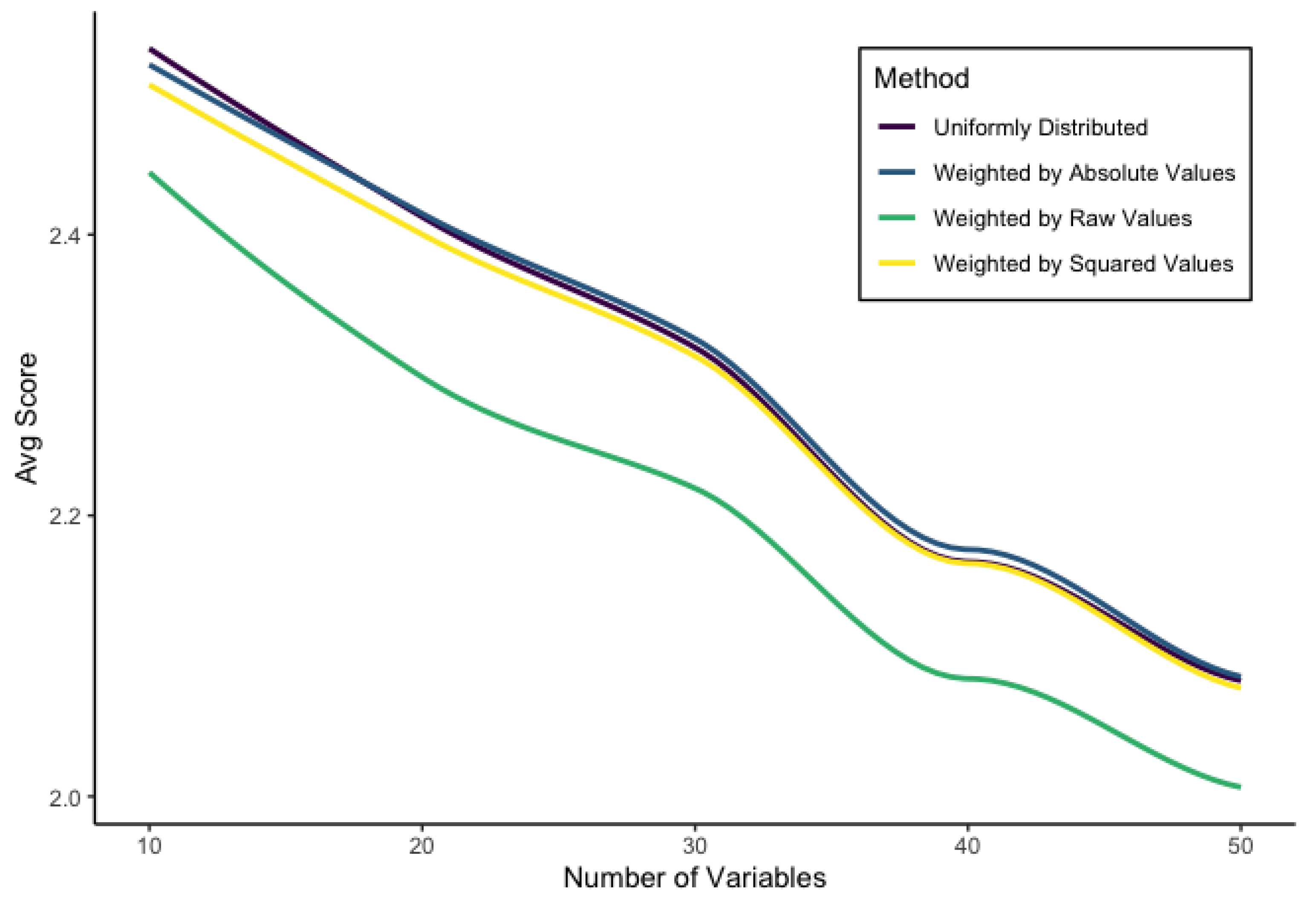
Since the initial simulation only used data with three explanatory variables, we have completed additional simulations with different numbers of variables. The goal of this is to ascertain that the weighted by absolute value is the best method no matter the number of variables.
Our additional simulations used between 10 and 50 covariates across over 250 combinations of y 1 , y 2 , θ 1 , and θ 2 . For these simulations, all of our covariates were distributed uniformly between 1 and 1. After performing the simulation, we saw that the absolute value method of weighting alpha is again the best (but just barely) based on overall score and in other metrics as well. The results are shown in Table A1.
Table A1. Results from additional simulations encompassing different numbers of variables and different variable values.
MethodScoreDirection
Score
Relative
Value Score
Rank ScorePct Same
Sign
Pct Same
Rank
Weighted by
Absolute Value
2.130.8840.7700.48074.4%24.9%
Uniformly
Distributed
2.130.8900.7660.47075.0%23.7%
Weighted by
Squared Value
2.120.8800.7680.47573.9%24.3%
Weighted by
Raw Value
2.000.7800.7530.46863.5%23.2%
Due to these results, we are assured that the absolute weighting method of distributing α is the best based on our chosen metrics, across different numbers of covariates. It can be seen in Figure A1 that the general score decreases as we add more variables. However, this is consistent with what we observed when we compared TreeSHAP (exact) to kernelSHAP (on singular models, not two-part models), as demonstrated in Figure A2.
Figure A1. How the number of covariates impacts overall score on average for mSHAP compared to kernelSHAP.
Risks 10 00003 g0a1
Figure A2. How the number of covariates impacts overall score, on average, for TreeSHAP compared to kernelSHAP.
Risks 10 00003 g0a2

Appendix D. The Data

The data used to create the model include a Property Damage dataset, which is not available publicly but can be obtained through the Casualty Actuarial Society.

Appendix E. The Model

Both the severity model and the frequency model were tuned in R using an h2o backend (H2O.ai 2021). Tuning parameters are given in Table A2, and model metrics are given in Table A3. All model metrics were computed on the test (hold-out) subset of data. These tuning results were then used to create the final model in Python using scikit-learn (Pedregosa et al. 2011). Scikit-learn was used to create the models because multinomial predictions do not have SHAP support in H 2 O as of the time of writing.
Table A2. Tuning parameters for the frequency and severity models.
Tuning ParameterSeverity ModelFrequency Model
ntrees200100
max_depth3020
mtries2020
min_split_improvement0.00010.001
sample_rate0.6320.632
Table A3. Model metrics for all models.
ModelMAEMSELogloss
Severity Model283216,359,170NA
Frequency ModelNA0.0740.427
Two-Part Model683830,351NA

Appendix F. Code Availability

The code used to tune the model (as well as additional code focused on working with the CAS datasets) can be found at this github link: https://github.com/srmatth/CAS (accessed 16 October 2021).
mSHAP has been developed into an R package as well. The R package can be downloaded from CRAN, with the R code of the following:
  • install.packages("mshap")
or the development version from https://github.com/srmatth/mshap (accessed 16 October 2021) can be obtained by running the following:
  • devtools::install_github("srmatth/mshap")
in R.
The mSHAP package repository (https://github.com/srmatth/mshap, accessed 16 October 2021) also contains all codes and data used to generate the plots in this paper, as well as the code used to run the various simulations mentioned. It can be found in the inst/paper directory under the main directory of the package. Be aware that installing the package by following the steps above will not download the code used in this paper; it must be obtained from the github repository.

References

  1. Ablad, Mouad, Bouchra Frikh, and Brahim Ouhbi. 2021. Uncertainty quantification in deep learning context: Application to insurance. Paper presented at 2020 6th IEEE Congress on Information Science and Technology (CiSt), Agadir and Essaouira, Morocco, June 5–12; pp. 110–15. [Google Scholar]
  2. Akinyemi, Kemi, and Ben Leiser. 2020. The Use of Advanced Predictive Analytics for Rate Making in Insurance. Available online: https://www.soa.org/globalassets/assets/library/newsletters/actuarial-technology-today/2020/may/att-2020-05.pdf (accessed on 8 June 2021).
  3. Arrieta, Alejandro Barredo, Natalia Díaz-Rodríguez, Javier Del Ser, Adrien Bennetot, Siham Tabik, Alberto Barbado, Salvador García, Sergio Gil-López, Daniel Molina, Richard Benjamins, and et al. 2020. Explainable artificial intelligence (xai): Concepts, taxonomies, opportunities and challenges toward responsible ai. Information Fusion 58: 82–115. [Google Scholar] [CrossRef] [Green Version]
  4. Doran, Derek, Sarah Schulz, and Tarek R Besold. 2017. What does explainable ai really mean? A new conceptualization of perspectives. arXiv arXiv:1710.00794. [Google Scholar]
  5. Frees, Edward W., and Yunjie Sun. 2010. Household life insurance demand: A multivariate two-part model. North American Actuarial Journal 14: 338–54. [Google Scholar] [CrossRef]
  6. Gómez-Déniz, Emilio, and Enrique Calderín-Ojeda. 2021. A priori ratemaking selection using multivariate regression models allowing different coverages in auto insurance. Risks 9: 137. [Google Scholar] [CrossRef]
  7. Gunning, David. 2017. Explainable artificial intelligence (xai). Defense Advanced Research Projects Agency (DARPA), ND Web 2: 2. [Google Scholar] [CrossRef] [PubMed] [Green Version]
  8. Heras, Antonio, Ignacio Moreno, and José L Vilar-Zanón. 2018. An application of two-stage quantile regression to insurance ratemaking. Scandinavian Actuarial Journal 9: 753–69. [Google Scholar] [CrossRef]
  9. H2O.ai. 2021. h2o R Package. Version 3.34.0.1. Mountain Viewm: H2O.ai, Inc. [Google Scholar]
  10. Li, Shoujun, Yanzi Miao, Guangyu Li, and Muhammad Ikram. 2020. A novel varistructure grey forecasting model with speed adaptation and its application. Mathematics and Computers in Simulation 172: 45–70. [Google Scholar] [CrossRef]
  11. Lipton, Zachary C. 2018. The mythos of model interpretability: In machine learning, the concept of interpretability is both important and slippery. Queue 16: 31–57. [Google Scholar] [CrossRef]
  12. Lundberg, Scott M., and Su-In Lee. 2017. A unified approach to interpreting model predictions. Paper presented at the 31st International Conference on Neural Information Processing Systems, Long Beach, CA, USA, December 4–9; pp. 4765–74. [Google Scholar]
  13. Lundberg, Scott M., Gabriel Erion, Hugh Chen, Alex DeGrave, Jordan M Prutkin, Bala Nair, Ronit Katz, Jonathan Himmelfarb, Nisha Bansal, and Su-In Lee. 2020. From local explanations to global understanding with explainable ai for trees. Nature Machine Intelligence 2: 56–57. [Google Scholar] [CrossRef] [PubMed]
  14. Pedregosa, Fabian, Gaël Varoquaux, Alexandre Gramfort, Vincent Michel, Bertrand Thirion, Olivier Grisel, Mthieu Blondel, Peter Prettenhofer, Ron Weiss, Vincent Dubourg, and et al. 2011. Scikit-learn: Machine learning in Python. Journal of Machine Learning Research 12: 2825–30. [Google Scholar]
  15. Prabowo, Agung, Mustafa Mamat, Sukono, and Afif Amrullah Taufiq. 2019. Pricing of Premium for Automobile Insurance using Bayesian Method. International Journal of Recent Technology and Engineering 8: 6226–29. [Google Scholar]
  16. Romaniuk, Maciej. 2017. Analysis of the insurance portfolio with an embedded catastrophe bond in a case of uncertain parameter of the insurer’s share. In Information Systems Architecture and Technology, Proceedings of 37th International Conference on Information Systems Architecture and Technology–ISAT 2016–Part IV, Karpacz, Poland, September 18–20. Berlin/Heidelberg: Springer, pp. 33–43. [Google Scholar]
  17. Shapley, Lloyd S. 1953. A value for n-person games. Contributions to the Theory of Games 2: 307–17. [Google Scholar]
  18. Slundberg. 2020. SHAP Values for Ensemble of XGBoost Models. Available online: https://github.com/slundberg/shap/issues/112 (accessed on 7 April 2021).
Figure 1. Heat maps for the λ functions. (a) Heatmap of λ 1 . (b) Heatmap of λ 2 .
Risks 10 00003 g001
Figure 2. How θ 1 impacts overall score on average.
Risks 10 00003 g002
Figure 3. How θ 2 impacts overall score on average.
Risks 10 00003 g003
Figure 4. Computational time of kernelSHAP and mSHAP. (a) Fixed n. (b) Fixed number of variables.
Risks 10 00003 g004
Figure 5. Example summary plots of SHAP values from the individual model parts. (a) Summary plot of the frequency model’s SHAP values for the 0 claim class. (b) Summary plot of the severity model’s SHAP values.
Risks 10 00003 g005
Figure 6. Summary plot of the two-part model’s mSHAP values.
Risks 10 00003 g006
Figure 7. Observation plot from the two-part model’s mSHAP values. This plot shows how mSHAP can be used to explain a single observation.
Risks 10 00003 g007
Table 1. Details of the scope of the simulation, describing all possible values for each variable.
VariablePossible Values
y 1 x 1 + x 2 + x 3
2 x 1 + 2 x 2 + 3 x 3
y 2 x 1 + x 2 + x 3
2 x 1 + 2 x 2 + 3 x 3
x 1 x 2 x 3
x 1 2 x 2 3 x 3 4
( x 1 + x 2 ) / ( x 1 + x 2 + x 3 )
x 1 x 2 / ( x 1 + x 1 x 2 + x 1 2 x 3 2 )
θ 1 1.5, 2.5, 3.5, 4.5, 5.5, 6.5, 7.5, 8.5, 9.5, 10.5,
11.5, 12.5, 13.5, 14.5, 15.5, 16.5, 17.5, 18.5, 19.5, 20.5
θ 2 1, 6, 11, 16, 21, 26, 31, 36, 41, 46
Table 2. Results of the simulation for different methods of distributing α , note that the highest score in each column is indicated with boldface type.
MethodScoreDirection
Score
Relative
Value Score
Rank ScorePct Same
Sign
Pct Same
Rank
Weighted by
Absolute Value
2.270.8690.5940.80284.8%62.5%
Weighted by
Squared Value
2.210.8410.5790.79281.8%60.8%
Uniformly
Distributed
2.200.8580.5630.78383.7%59.4%
Weighted by
Raw Value
1.990.7270.4940.76871.4%56.2%
Publisher’s Note: MDPI stays neutral with regard to jurisdictional claims in published maps and institutional affiliations.