Lévy Interest Rate Models with a Long Memory

Abstract

This article proposes an interest rate model ruled by mean reverting Lévy processes with a sub-exponential memory of their sample path. This feature is achieved by considering an Ornstein–Uhlenbeck process in which the exponential decaying kernel is replaced by a Mittag–Leffler function. Based on a representation in term of an infinite dimensional Markov processes, we present the main characteristics of bonds and short-term rates in this setting. Their dynamics under risk neutral and forward measures are studied. Finally, bond options are valued with a discretization scheme and a discrete Fourier’s transform.

1. Introduction

From the 1980s to current years, many interest rate models were proposed in the literature. Their common aim is to explain changes in bond or swap quotes and to replicate risks within the interest rates market. Three dominating frameworks coexist: short-term rate, forward rate and the Libor market models. In this last approach proposed by Brace et al. (1997), interest rates are driven by geometric processes. In the forward rate model pioneered by Heath et al. (1992), the term structure of rates is specified through instantaneous forward rates. Mercurio and Moraleda (2000) and Falini (2010) proposed a forward model with a humped structure of volatilities. Li et al. (2020) developed a forward rate model unifying most existing Gaussian models for interest rates. Short-term rate models such as those promoted by Hull and White (1990) specify a mean reverting dynamic for the instantaneous risk-free rate. The framework developed in this article belongs to this third category.

The family of short-term rate models gathers multiple frameworks and we refer the reader, e.g., to Boero and Torricelli (1996) or to Schmidt (2011) for a review. On the other hand, various processes were proposed to explain the interest rate risk. The literature is too vast to be exhaustive. We restrict our attention to contributions related to this work and do not attempt at providing a general overview, referring instead to Brigo and Mercurio (2006) for detailed accounts on the topic. For instance, Eberlein and Raible (1999) were among the first to propose a short-term rate model driven by Lévy processes. In their setting, the short-term rate is ruled by Ornstein–Uhlenbeck processes reverting in an exponential manner to a mean level. Within this framework, Eberlein and Kluge (2005) derived analytical formulae for the prices of caps and floors using bilateral Laplace transforms. In a similar setting, Hainaut and MacGilchrist (2010) proposed a pentanomial tree for pricing derivatives. Hainaut (2013) studied the properties of a Gaussian short-term rate with a Markov Switching Multifractal volatility. Moreno and Platania (2015) proposed a square-root model replicating economic cycles in the dynamics of interest rates. Hainaut (2016) and Njike and Hainaut (2020) developed unicurve and multicurve models in which the short-term rate is exposed to self-excitating jumps. Fontana et al. (2020) studied a modelling framework exploiting the the self-exciting behavior of continuous-state branching processes with immigration (CBI).

A wide majority of short-term rate models are driven by Markov mean reverting processes. In this setting, the interest rate depends on its path through the integral of past occurrences weighted by an exponential decaying function, called the memory kernel. In this framework, the influence of previous variations of interest rates decreases exponentially over time. In this article, we consider an alternative that consists in replacing this memory kernel by a Mittag–Leffler decaying function. This function is sub-exponential and may be seen as a generalization of the exponential. In this setting, the interest rate remembers its previous occurrences for a longer period than in the exponential framework. The motivations for studying such a model are multiple. Firstly, the features replicate the persistence empirically observed in short term rates, as illustrated in Section 3, or in nominal yields and inflation, as shown by Golinski and Zaffaroni (2016). Secondly, the proposed model has a sufficient level of analytical tractability for most of financial applications such as option pricing. Finally, it also offers a novel alternative to existing approaches based on the fractional Brownian motion for introducing long memory, as for instances studied in Cheridito et al. (2003) or Maejima and Yamamoto (2003).

A consequence of this change of memory kernel is that the interest rate process is not Markovian anymore. Bond prices depend then on the sample path of past rates. Nevertheless, we take advantage of the representation of the memory kernel as a Laplace Stieltjes integral to rewrite the short-term rate as an infinite dimensional Markov process. The last part of the article studies the properties of the model under a forward measure and proposes a pricing method for bond options.

2. A Lévy Model with a Mittag Leffler Kernel

We consider that the short-term rate is driven by $d\in \mathbb{N}$ independent Lévy processes, denoted by ${\left(L_t^{\left(j\right)}\right)}_{t\ge 0}$ for $j=1,\dots ,d$. These processes are defined on a probability space $\mathsf{\Omega },$ endowed with the natural filtration ${\left({\mathcal{F}}_t\right)}_{t\ge 0}$ and a risk neutral measure, $\mathbb{Q}$. Each process ${\left(L_t^{\left(j\right)}\right)}_{t\ge 0}$ has independent and stationary increments. It is fully described by a triplet $\left({\mu }_j,{\sigma }_j^2,{\nu }_j\right)$ where ${\mu }_j\in \mathbb{R}$, ${\sigma }_j\in {\mathbb{R}}^{+}$ and ${\nu }_j(.)$ is a Lévy measure. The moment generating function (mgf) is denoted by ${\varphi }_t^{\left(j\right)}\left(\omega \right)$ for $j=1,\dots ,d$ and is equal to the following:

$$\begin{array}{ccc}\hfill {\varphi }_t^{\left(j\right)}\left(\omega \right)& :=& \mathbb{E}\left(exp\left(\omega (L_t^{\left(j\right)}-L_0^{\left(j\right)})\right)|{\mathcal{F}}_0\right)\hfill \\ & =& exp\left(t\left({\mu }_j\omega +\frac{1}{2}{\omega }^2{\sigma }_j^2+{\int }_{\mathbb{R}}\left(e^{\omega z}-1-\omega z{1}_{\left|z\right|<ϵ}\right){\nu }_j\left(dz\right)\right)\right)\hfill \\ & =& exp\left(t{\psi }_j\left(\omega \right)\right),\hfill \end{array}$$

(1)

where $ϵ>0$. Notice that if the Lévy measure, ${\nu }_j(.)$, has no singurality at $z=0$, we can set $ϵ$ to zero. The function ${\psi }_j\left(\omega \right)$ is the characteristic exponent of this Lévy process that is always defined for pure imaginary numbers. Without loss of generality, we assume that $L_0^{\left(j\right)}=0$. According to the Lévy Itô decomposition, each $L_t^{\left(j\right)}$ is the sum of three components: a deterministic drift ${\mu }_{j}t$, a Brownian motion with variance ${\sigma }_j^2$ and a jump process, $J_j(t,z)$, of intensity ${\nu }_j\left(dz\right)$ well defined on $[-\infty ,0)\cup (0,+\infty ]$. This Lévy measure is such that the probability of observing k jumps between $[{\tau }_1,{\tau }_2]$ of a size included in a set $B\subset {\mathbb{R}}_{\backslash \left\{0\right\}}$ is given by the following:

$$\begin{array}{ccc}\hfill P\left(J_j([{\tau }_1,{\tau }_2]\times B)=k\right)& =& e^{-{\int }_{{\tau }_1}^{{\tau }_2}{\int }_B{\nu }_j\left(dz\right)dt}\frac{{\left({\int }_{{\tau }_1}^{{\tau }_2}{\int }_B{\nu }_j\left(dz\right)dt\right)}^k}{k!},\hfill \end{array}$$

(2)

for $j=1,\dots ,d$. If ${\left(W_t^{\left(j\right)}\right)}_{t\ge 0}$ for $j=1,\dots ,d$, are independent Brownian motions on $\left(\mathsf{\Omega },\mathcal{F},\mathbb{Q}\right)$, $L_t^{\left(j\right)}$ may be split as the sum of a drift, a Brownian motion and a jump process:

$$d{L}_t^{\left(j\right)}={\mu }_{j}dt+{\sigma }_{j}d{W}_t^{\left(j\right)}+{\int }_{\mathbb{R}}z{\tilde{J}}_j(dt,dz),$$

(3)

where the following is the case.

$${\tilde{J}}_j(dt,dz)=J_j(dt,dz)-{\mathbf{1}}_{\left|z\right|<ϵ}{\nu }_j\left(dz\right)dt.$$

Without loss of generality, we assume that $\mathbb{E}\left(L_t^{\left(j\right)}\right)=0$. This constraint implies that the drift compensates jumps larger than $ϵ$ in absolute value:

$$\begin{array}{ccc}\hfill {\mu }_j& =& -{\int }_{\left|z\right|\ge ϵ}z{\nu }_j\left(dz\right),j=1,\dots ,d.\hfill \end{array}$$

From Cont and Tankov (2003, Lemma 15.1, p. 482), for any integrable function $f:\mathbb{R}\to \mathbb{C}$, the following relation holds.

$$\mathbb{E}\left(e^{\omega {\int }_s^{t}f\left(u\right)d{L}_u^{\left(j\right)}}|{\mathcal{F}}_s\right)=exp\left({\int }_s^t{\psi }_j\left(\omega f\left(u\right)\right)du\right),j=1,\dots ,d.$$

(4)

This can be proved by approaching $f(.)$ with a stepwise function and by using the property of independence of increments. This property will be useful in later developments. We postulate that the risk-free rate, ${\left(r_t\right)}_{t\ge 0}$, is the sum of a deterministic function $\phi \left(t\right):\mathbb{R}\to \mathbb{R}$ and of d processes: ${\left(X_t^{\left(d\right)}\right)}_{t\ge 0}$:

$$r_t=\phi \left(t\right)+\sum _{j=1}^d{X}_t^{\left(j\right)},$$

(5)

where $X_t^{\left(j\right)}$ is such that the following is the case.

$$X_t^{\left(j\right)}=g_j\left(t\right)X_0^{\left(j\right)}+{\int }_0^t{g}_j(t-u)d{L}_u^{\left(j\right)}.$$

(6)

The function $g_j(.):{\mathbb{R}}^{+}\to \mathbb{R}$ is continuously decreasing with an initial value $g_j\left(0\right)=1$. As $g_j(.)$ determines the influence of past realizations of $L_t^{\left(j\right)}$ on the current value of the process, we call it “memory kernel” or “kernel function” in the remainder of this article. When the function $g_j\left(t\right)$ decreases exponentially, the processes ${\left(X_t^{\left(j\right)}\right)}_{j=1,\dots ,d}$ are Markov and mean-reverting as recalled in Appendix A. Such a model was, e.g., developed in Hainaut and MacGilchrist (2010) for pricing interest rate derivatives and will serve as benchmark in numerical illustrations. However, ${\left(X_t^{\left(j\right)}\right)}_{t\ge 0}$ and ${\left(r_t\right)}_{t\ge 0}$ are in general not Markov for any other non-exponential kernels. This feature makes difficult the evaluation of bond prices at a given time $t>0$ as their value depends on the entire sample path of interest rates up to t. Nevertheless, for a few kernel functions that admit a representation as a Laplace–Stieltjes integral, we will show that the interest rate may be represented as an infinite dimensional Markov process. In particular, we consider two types of kernel functions, both based on the Mittag–Leffler function, denoted by $E_{\alpha }(.)$ where $\alpha \in [0,1]$.

$$g_j\left(t\right)=E_{{\alpha }_j}(-{\beta }_{j}t)\mathrm{or}{g}_j\left(t\right)=E_{{\alpha }_j}(-{\beta }_j{t}^{{\alpha }_j}).$$

(7)

In order to understand the motivation for working with such functions, we need to review the main properties of the Mittag–Leffler function. The Mittag–Leffler function of order $\alpha >0$ plays a fundamental role in the fractional calculus and can be considered as an extension of the exponential function. It is defined as an infinite sum.

$$E_{\alpha }\left(t\right)=\sum _{n=0}^{\infty }\frac{t^n}{\mathsf{\Gamma }(n\alpha +1)}.$$

In this article, we assume that $\alpha \in [0,1]$. For this range of values, $E_{\alpha }(-t)$ is an intermediary between the power and the exponential decreasing functions.

$$E_0\left(-t\right)=\frac{1}{1+t}\forall \left|t\right|<1\mathrm{and}{E}_1(-t)=e^{-t}.$$

We refer the reader to the book of Gorenflo et al. (2020) for a detailed presentation of this function. For a complete presentation of fractional calculus, we recommend the book of Baleanu et al. (2012) and the book of Kochubei and Luchko (2019). Let us recall that a function $f:(0,\infty )\to \infty$ is called completely monotonic if it possesses derivatives $f^{\left(n\right)}\left(t\right)$ of any order $n=0,1,2\dots$ and the derivatives are alternating in sign.

$${\left(-1\right)}^n{f}^{\left(n\right)}\left(t\right)\ge 0\forall t\in ((0,\infty ).$$

The above property is equivalent to the existence of a representation of the function f in the form of a Laplace–Stieltjes integral with non-decreasing density and non-negative measure $d\gamma (.)$ such that the following is the case.

$$f\left(t\right)={\int }_0^{\infty }{e}^{-ut}d\gamma \left(u\right).$$

The Mittag–Leffler function of negative argument $E_{\alpha }(-\beta t)$ is completely monotonic for all $0\le \alpha \le 1$ and $\beta \in {\mathbb{R}}^{+}$. A proof of this result is available in Gorenflo et al. (2020) on page 47. The authors show the following:

$$\begin{array}{ccc}\hfill E_{\alpha }(-\beta t)& =& {\int }_0^{\infty }{e}^{-tu}d{\gamma }_{\alpha ,\beta }\left(u\right),\hfill \end{array}$$

(8)

where the derivative of ${\gamma }_{\alpha ,\beta }\left(u\right)$ is equal to the following.

$$\begin{array}{ccc}\hfill \frac{d{\gamma }_{\alpha ,\beta }\left(u\right)}{du}& =& \frac{1}{\pi \alpha }\sum _{k=1}^{\infty }\frac{{\left(-1\right)}^{k-1}}{k!}sin\left(\pi \alpha k\right)\mathsf{\Gamma }(\alpha k+1)\frac{u^{k-1}}{{\beta }^k}.\hfill \end{array}$$

(9)

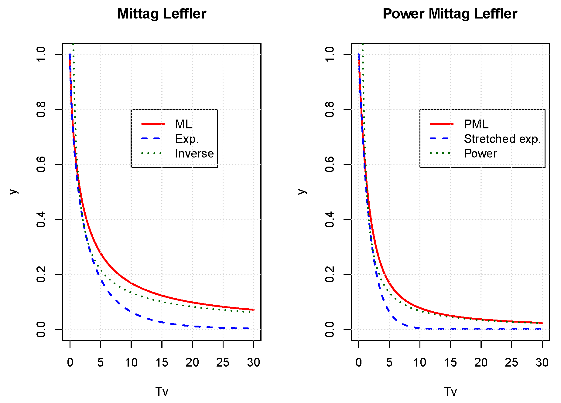
Given that $E_{\alpha }\left(0\right)=1$, we have ${\int }_0^{\infty }d{\gamma }_{\alpha ,\beta }\left(u\right)=1$ and ${\gamma }_{\alpha ,\beta }(.)$ is then a measure of probability on ${\mathbb{R}}^{+}$. In the remainder of this article, $E_{\alpha }(-\beta t)$ is called the decreasing Mittag–Leffler (ML) kernel. The DML behaves at short-term as follows:

$$\begin{array}{ccc}\hfill E_{\alpha }(-\beta t)& =& 1-\frac{\beta t}{\mathsf{\Gamma }(1+\alpha )}+\dots \sim exp\left(-\frac{\beta t}{\mathsf{\Gamma }(1+\alpha )}\right),\hfill \end{array}$$

when $t\to 0$. From Haubold et al. (2011), we known that when $t\to \infty$, DML converges to the following.

$$E_{\alpha }(-\beta t)\sim \frac{{\left(\beta t\right)}^{-1}}{\mathsf{\Gamma }\left(1-\alpha \right)}.$$

The function $E_{\alpha }(-\beta t)$ interpolates for intermediate times t between the decreasing exponential and the inverse power law. The exponential models fast decay for small time t, whereas the asymptotic inverse power law entails a slow decrease at long term. This point is illustrated in the left plot of Figure 1, which compares the ML kernel to the exponential and inverse power functions.

The Mittag–Leffler function is also related to the fractional calculus. In order to explain this link, we recall that Caputo’s fractional derivative of order $\alpha \in (0,1)$ for a function $h\left(t\right)$: ${\mathbb{R}}^{+}\to \mathbb{R}$, ${\mathcal{C}}^1$ with respect to t is defined by the following.

$$\begin{array}{ccc}\hfill \frac{{\partial }^{\alpha }}{\partial t^{\alpha }}h\left(t\right)& =& \frac{1}{\mathsf{\Gamma }(1-\alpha )}{\int }_0^t{\left(t-s\right)}^{-\alpha }\frac{\partial }{\partial s}h\left(s\right)ds\hfill \end{array}$$

(10)

When $\alpha =1$, this derivative corresponds to the first order derivative. The solution of the fractional differential equation of the following:

$$\frac{{\partial }^{\alpha }}{\partial t^{\alpha }}y\left(t\right)=-\beta y\left(t\right)0<\alpha <1$$

with the initial condition $y\left(0\right)=b_0$ is $y\left(t\right)=E_{\alpha }(-\beta t^{\alpha })$. We abusively call this function the power decreasing Mittag–Leffler kernel (PML). The Laplace transform of $E_{\alpha }(-\beta t^{\alpha })$ is given by $\frac{s^{\alpha -1}}{s^{\alpha }+\beta }$ where ${Re\left(s\right)>\left|\beta \right|}^{\frac{1}{\alpha }}$. By inverting this transform, we can prove as in Gorenflo and Mainardi (1997) that the PML is the Laplace transform of the following:

$$E_{\alpha }(-\beta t^{\alpha })={\int }_0^{\infty }{e}^{-ut}d{\gamma }_{\alpha ,\beta }^p\left(u\right),$$

(11)

where the derivative of ${\gamma }_{\alpha ,\beta }^p\left(u\right)$ is given by the following.

$$\frac{d{\gamma }_{\alpha ,\beta }^p\left(u\right)}{du}=\frac{1}{\pi }\frac{\beta u^{\alpha -1}sin\left(\alpha \pi \right)}{u^{2\alpha }+2\beta u^{\alpha }cos\left(\alpha \pi \right)+{\beta }^2}.$$

(12)

Since $E_{\alpha }\left(0\right)=1$, we have ${\int }_0^{\infty }d{\gamma }_{\alpha ,\beta }^p\left(u\right)=1$ and ${\gamma }_{\alpha ,\beta }^p\left(u\right)$ is a measure of probability on ${\mathbb{R}}^{+}$. As underlined by Mainardi (2020), the PML behaves at short-term as follows:

$$\begin{array}{ccc}\hfill E_{\alpha }(-\beta t^{\alpha })& =& 1-\frac{\beta t^{\alpha }}{\mathsf{\Gamma }(1+\alpha )}+\dots \sim exp\left(-\frac{\beta t^{\alpha }}{\mathsf{\Gamma }(1+\alpha )}\right).\hfill \end{array}$$

when $t\to 0$. From Erdélyi et al. (1955), we known that when $t\to \infty$, PML converges to the following.

$$E_{\alpha }(-\beta t^{\alpha })\sim \frac{{\left({\beta }^{1/\alpha }t\right)}^{-\alpha }}{\mathsf{\Gamma }\left(1-\alpha \right)}.$$

As a consequence, the function $E_{\alpha }(-\beta t^{\alpha })$ interpolates for intermediate times t between the stretched exponential and the negative power law. The stretched exponential models the very fast decay at short-term whereas the asymptotic power law is due to the very slow decay for large time t. The right plot of Figure 1 illustrates this convergence.

Figure 2 presents simulated sample paths of the short-term rate with a one dimensional ($d=1$) model ruled by a Brownian motion. These paths are computed for various $\alpha$ with the same random occurrences in order to make a comparison feasible. For the ML kernel, the trajectories are nearly similar. An analysis of figures reveals that the sample path is smoother for $\alpha =0.50$ than for $\alpha =0.90$. This trend becomes visible if we choose the highest value for $\beta$. For PML sample paths, the difference is clearly visible. Decreasing $\alpha$ reduces the volatility of rates and smooths the sample path.

To conclude this section, we present the first two moments of the short-term rate and its autocovariance function. The ML and PML kernels defined in Equation (7) are continuously decreasing and integrable functions on any bounded interval of $\mathbb{R}$. From Equation (4), the mgf of $X_t^{\left(j\right)}$ for $j=1,\dots ,d$ is then equal to the following.

$$\begin{array}{ccc}\hfill \mathbb{E}\left(e^{\omega X_t^{\left(j\right)}}|{\mathcal{F}}_0\right)& =& exp\left(\omega g_j\left(t\right)X_0^{\left(j\right)}+{\int }_0^t{\psi }_j\left(\omega g_j(t-u)\right)du\right).\hfill \end{array}$$

Deriving mgf allows us to find the first moments of $X_t^{\left(j\right)}$ conditionally to the initial information. On the other hand, from the following representation:

$$r_t=\phi \left(t\right)+\sum _{j=1}^d{g}_j\left(t\right)X_0^{\left(j\right)}+\sum _{j=1}^d{\int }_0^s{g}_j(t-u)d{L}_u^{\left(j\right)}+\sum _{j=1}^d{\int }_s^t{g}_j(t-u)d{L}_u^{\left(j\right)},$$

(13)

of $r_t$, we infer that the conditional expectation of the short-term rate is given by the following.

$$\begin{array}{cc}\hfill \mathbb{E}\left(r_t|{\mathcal{F}}_s\right)& =\phi \left(t\right)+\sum _{j=1}^d{g}_j\left(t\right)X_0^{\left(j\right)}+\sum _{j=1}^d{\int }_0^s{g}_j(t-u)d{L}_u^{\left(j\right)},\hfill \end{array}$$

(14)

On the other hand, the conditional variance of $r_t$ is equal to the sum of variances of Lévy processes times the integral of the squared kernels.

$$\begin{array}{cc}\hfill \mathbb{V}\left(r_t|{\mathcal{F}}_s\right)& =\sum _{k=1}^d\left({\sigma }_j^2+{\int }_{\mathbb{R}}{z}^2{\nu }_j\left(dz\right)\right){\int }_s^t{g}_j{(t-u)}^{2}du.\hfill \end{array}$$

(15)

Unfortunately the integral of $g_j{(.)}^2$ does not admit a closed form expression for the ML and PML kernels. Nevertheless, they can be numerically estimated. A direct calculation allows us to infer that autocovariance between $r_t$ and $r_u$ for $u\le t$ is given by:

$$\begin{array}{ccc}\hfill \mathbb{C}\left(r_t{r}_u|{\mathcal{F}}_s\right)& =& \sum _{k=1}^d\mathbb{E}\left({\int }_s^t{g}_j(t-v)d{L}_v^{\left(j\right)}{\int }_s^u{g}_j(u-v)d{L}_v^{\left(j\right)}\right)\hfill \\ & =& \sum _{k=1}^d\left({\sigma }_j^2+{\int }_{\mathbb{R}}{z}^2{\nu }_j\left(dz\right)\right){\int }_s^u{g}_j(t-v)g_j(u-v)dv.\hfill \end{array}$$

(16)

Contrary to the exponential case, this covariance function between $r_t$ and $r_{t-\Delta }$ does not admit any closed form expression when $t\to \infty$.

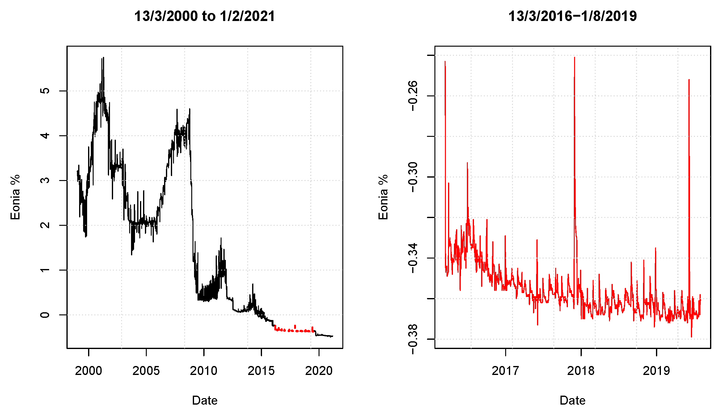
3. Empirical Motivation

This short section provides some empirical arguments motivating the developments performed in this article, particularly the choice of a ML or PML memory kernel. We fit univariate Gaussian models ($d=1$) with exponential ML and PML kernels to the Eonia time series from 13 March 2016 to 1 August 2019. The dataset counts $n_{obs}=$ 866 daily observations. We select this time window mainly because Eonia was relatively stable during this period, as illustrated in the right plot of Figure 3. This allows us to assume that the trend function, $\phi \left(t\right)$, is constant. Considering a larger dataset would raise the question of modelling a non-linear trend in view of the left plot of Figure 3.

The dates of observations are denoted by $t_0,t_1,\dots ,t_{n_{obs}-1}$, whereas the step of time between two successive observations is ${\Delta }_t$. We first consider a one dimensional exponential kernel model as detailed in Appendix A. Under the assumption that $\phi \left(t_k\right)=\phi (t_k+{\Delta }_t)$ and $X_0=0$, we find the following:

$$\begin{array}{ccc}\hfill \Delta L_{k+1}& =& L_{t_{k+1}}-L_{t_k}\approx r_{t_{k+1}}-r_{t_k}-\sum _{j=0}^k\left(e^{-\kappa (t_{k+1}-t_j)}-e^{-\kappa (t_k-t_j)}\right)\Delta L_j,\hfill \end{array}$$

for $k=1,\dots ,n_{obs}-1$. Under the assumption that $L_t$ is a Brownian motion without drift and of variance ${\sigma }^2$, parameters are estimated by log-likelihood maximization. We next consider models with ML and PML kernel functions. In this cases, the variations of the underlying Lévy process are approached by the following:

$$\begin{array}{ccc}\hfill \Delta L_{k+1}& =& L_{t_{k+1}}-L_{t_k}\approx r_{t_{k+1}}-r_{t_k}-\sum _{j=0}^k\left(g(t_{k+1}-t_j)-g(t_k-t_j)\right)\Delta L_j,\hfill \end{array}$$

for $k=1,\dots ,n_{obs}-1$ where $g(.$) is either the ML or the PML function. Under the assumption of normality, parameters are estimated by log-likelihood maximization whereas the goodness of fit is measured with the Akaike Information Criterion (AIC). The results of this procedure are reported in

Table 1. Parameter estimates by log-likelihood maximization of one dimensional models with exponential, ML and PML kernels.

	Exponential		ML	PML
$\sigma$	1.4763 × ${10}^{-3}$	$\sigma$	1.4767 × ${10}^{-3}$	1.3927× ${10}^{-3}$
$\kappa$	0.6926	$\alpha$	0.9954	0.1924
		$\beta$	0.7218	1.2171
Log-likelihood	6809.75	Log-likelihood	6809.93	6861.15
AIC	−13,615.50		−13,613.86	−13,716.30

. In terms of log-likelihood, exponential and ML models achieve the same goodness of fit but the exponential model is more parsimonious and preferred. They share the same estimated volatilities but the parameters of reversion $\kappa$ and $\beta$ slightly differ. The best fit, based on the AIC, is obtained with a power Mittag–Leffler kernel. The parameter $\alpha$ that drives the decay of the memory is small. This means that the process has a longer-term memory than the exponential model. On the other hand, the mean reversion speed is significantly higher than the ones of other models. We recall to the reader that estimated parameters reflect the dynamic of $r_t$ under the real measure $\mathbb{P}$ and not the risk neutral one.

4. Alternative Formulation

If the memory is not exponential decaying, the interest rate process ${\left(r_t\right)}_{t\ge 0}$ is not Markovian. This feature makes difficult the evaluation of bond prices or interest rate derivatives because their values depend on the entire history of the rate process. Nevertheless, if the memory kernel admits a representation as a Laplace–Stieltjes integral, we can convert the short-term rate into an infinite dimensional Markov process. Approximating this process allows us to infer the dynamic of bond prices. As developments are similar in both cases, we denote by ${\gamma }_j(.)$ the measures ${\gamma }_{{\alpha }_j,{\beta }_j}^{\left(j\right)}(.)$ or ${\gamma }_{{\alpha }_j,{\beta }_j}^{p\left(j\right)}(.)$ of $E_{{\alpha }_j}(-{\beta }_{j}t)$ and $E_{{\alpha }_j}(-{\beta }_j{t}^{{\alpha }_j})$. Let us recall that the function $g_j\left(t\right)=$${\int }_0^{\infty }{e}^{-\xi t}d{\gamma }_j\left(\xi \right)$. Using the Fubini’s theorem, the processes $X_t^{\left(j\right)}$ are then rewritten as follows:

$$\begin{array}{cc}\hfill X_t^{\left(j\right)}& =X_0^{\left(j\right)}{\int }_0^{\infty }{e}^{-t\xi }d{\gamma }_j\left(\xi \right)+{\int }_0^t{\int }_0^{\infty }{e}^{-\xi (t-u)}d{\gamma }_j\left(\xi \right)d{L}_u^{\left(j\right)}\hfill \\ \hfill & ={\int }_0^{\infty }\underset{Y_t^{(j,\xi )}}{\underbrace{\left(e^{-t\xi }{Y}_0^{(j,\xi )}+{\int }_0^t{e}^{-\xi (t-u)}d{L}_u^{\left(j\right)}\right)}}d{\gamma }_j\left(\xi \right)\hfill \end{array}$$

for $j=1,\dots ,d$. The $Y_t^{(j,\xi )}$ are Ornstein–Uhlenbeck processes for $j=1,\dots ,d$ and for all $\xi \in {\mathbb{R}}^{+}$. Their initial values are $X_0^{\left(j\right)}=Y_0^{(j,\xi )}$, and they obey to the following stochastic differential equation (SDE).

$$d{Y}_t^{(j,\xi )}=-\xi Y_t^{(j,\xi )}dt+d{L}_t^{\left(j\right)}.$$

(17)

As this SDE admits the following solution:

$$\begin{array}{cc}\hfill Y_t^{(j,\xi )}& =e^{-\xi (t-s)}{Y}_s^{(j,\xi )}+{\int }_s^t{e}^{-\xi (t-u)}d{L}_u^{\left(j\right)},\hfill \end{array}$$

(18)

the short-term rate is then a sum of integrals of $Y_t^{(j,\xi )}$.

$$r_t=\phi \left(t\right)+\sum _{j=1}^d{\int }_0^{\infty }{Y}_t^{(j,\xi )}d{\gamma }_j\left(\xi \right).$$

(19)

Given that ${\gamma }_{{\alpha }_j,{\beta }_j}^{\left(j\right)}(.)$ and ${\gamma }_{{\alpha }_j,{\beta }_j}^{p\left(j\right)}(.)$ are probability measures, the differential of $r_t$ is, on the other hand, equal to the following.

$$\begin{array}{cc}\hfill d{r}_t& =d\phi \left(t\right)-\sum _{j=1}^d{\int }_0^{\infty }\xi Y_t^{(j,\xi )}d{\gamma }_j\left(\xi \right)+\sum _{j=1}^d\underset{=1}{\underbrace{{\int }_0^{\infty }d{\gamma }_j\left(\xi \right)}}d{L}_t^{\left(j\right)}.\hfill \end{array}$$

Combining Equations (18) and (19) allows us to rewrite the short-term rate as the following sum:

$$\begin{array}{cc}\hfill r_t& =\phi \left(t\right)+\sum _{j=1}^d{\int }_0^{\infty }\left(e^{-\xi (t-s)}{Y}_s^{(j,\xi )}+{\int }_s^t{e}^{-\xi (t-u)}d{L}_u^{\left(j\right)}\right)d{\gamma }_j\left(\xi \right)\hfill \\ \hfill & =\phi \left(t\right)+\sum _{j=1}^d{\int }_0^{\infty }{e}^{-\xi (t-s)}{Y}_s^{(j,\xi )}d{\gamma }_j\left(\xi \right)+\sum _{j=1}^d{\int }_s^t{g}_j(t-u)d{L}_u^{\left(j\right)}\hfill \end{array}$$

(20)

which does not depend anymore upon information prior to s. This relation emphasizes that $r_t$ and ${\left(Y_t^{(j,\xi )}\right)}_{\xi \in {\mathbb{R}}^{+},j\in \{1,\dots ,d\}}$ form well an infinite dimensional Markov process. If we remember that $\mathbb{E}\left(L_t^{\left(j\right)}\right)=0$, we infer an equivalent representation of Equation (14) for the conditional expectation of $r_t$ in terms of $Y_t^{(j,\xi )}$.

$$\begin{array}{ccc}\hfill \mathbb{E}\left(r_t|{\mathcal{F}}_s\right)& =& \phi \left(t\right)+\sum _{j=1}^d{\int }_0^{\infty }{e}^{-\xi (t-s)}{Y}_s^{(j,\xi )}d{\gamma }_j\left(\xi \right).\hfill \end{array}$$

We will explain in the next section how to approximate the infinity of processes by discretizing measures ${\gamma }_j\left(\xi \right)$. However, we evaluate zero coupon bonds and instantaneous forward rates in this setting first.

5. Bond Prices and Forward Rates

A zero-coupon bond of maturity t delivers a unit cash-flow at expiry. Its price at time s prior to t is denoted by $P(s,t)$ and in absence of arbitrage, and it is the expected discount factor under the risk neutral measure, $P(s,t)=\mathbb{E}\left(e^{-{\int }_s^t{r}_{u}du}|{\mathcal{F}}_s\right)$. The next proposition presents a semi-closed form expression for this price.

Proposition 1.

Let us, respectively, define functions $B^{\left(\xi \right)}(s,t)$ and $h_j(s,t)$ as follows:

$$\begin{array}{ccc}\hfill B^{\left(\xi \right)}(s,t)& =& \frac{1}{\xi }\left(1-e^{-\xi (t-s)}\right),\hfill \end{array}$$

(21)

$$\begin{array}{cc}\hfill h_j(s,t)& ={\int }_0^{\infty }{B}^{\left(\xi \right)}(s,t)d{\gamma }_j\left(\xi \right),\hfill \end{array}$$

(22)

for $s\le t$ and $j=1,\dots ,d$. The zero coupon bond price is equal. to

$$\begin{array}{ccc}& & P(s,t)=exp\left(-{\int }_s^t\phi \left(u\right)du+\sum _{j=1}^d{\int }_s^t{\psi }_j(-h_j(u,t))du\right.\hfill \\ & & \left.-\sum _{j=1}^d\left(X_0^{\left(j\right)}{\int }_s^t{g}_j\left(u\right)du+{\int }_0^s{\int }_0^{\infty }{e}^{-\xi (s-u)}{B}^{\xi }(s,t)d{\gamma }_j\left(\xi \right)d{L}_u^{\left(j\right)}\right)\right).\hfill \end{array}$$

(23)

Proof. 

From Equation (13), we infer, after a change of the integration order, the following.

$$\begin{array}{cc}\hfill & {\int }_s^t{r}_{u}du={\int }_s^t\phi \left(u\right)du+\sum _{j=1}^d{X}_0^{\left(j\right)}{\int }_s^t{g}_j\left(u\right)du+\hfill \\ \hfill & \sum _{j=1}^d{\int }_0^s{\int }_s^t{g}_j(u-v)dud{L}_v^{\left(j\right)}+\sum _{j=1}^d{\int }_s^t{\int }_v^t{g}_j(u-v)dud{L}_v^{\left(j\right)}.\hfill \end{array}$$

A direct calculation allows us to rewrite the integrals of $g_j(.)$ in this last expression as follows.

$$\begin{array}{cc}\hfill {\int }_s^t{g}_j(u-v)du& ={\int }_0^{\infty }{e}^{-\xi (s-v)}{B}^{\xi }(s,t)d{\gamma }_j\left(\xi \right),\hfill \\ \hfill {\int }_v^t{g}_j(u-v)du& ={\int }_0^{\infty }{B}^{\xi }(v,t)d{\gamma }_j\left(\xi \right)=h_j(v,t).\hfill \end{array}$$

The zero-coupon bond price becomes the following.

$$\begin{array}{ccc}& & \mathbb{E}\left(e^{-{\int }_s^t{r}_{u}du}|{\mathcal{F}}_s\right)=\mathbb{E}\left(exp\left(-\sum _{j=1}^d{\int }_s^t{h}_j(v,t)d{L}_v^{\left(j\right)}\right)|{\mathcal{F}}_s\right)\times \hfill \\ & & exp\left(-{\int }_s^t\phi \left(u\right)du-\sum _{j=1}^d\left(X_0^{\left(j\right)}{\int }_s^t{g}_j\left(u\right)du+{\int }_0^s{\int }_0^{\infty }{e}^{-(s-v)}{B}^{\xi }(s,t)d{\gamma }_j\left(\xi \right)d{L}_v^{\left(j\right)}\right)\right).\hfill \end{array}$$

Finally, the expectation in this last expression is calculated with Equation (4). □

Remark that ${lim}_{\xi \to \infty }{B}^{\left(\xi \right)}(v,t)=0$ and that ${lim}_{\xi \to 0}{B}^{\left(\xi \right)}(v,t)=t-v$. Furthermore, the function $B^{\left(\xi \right)}(v,t)$ admits a single maximum ${\xi }^{*}<\infty$ such that $B^{\left({\xi }^{*}\right)}(v,t)\ge B^{\left(\xi \right)}(v,t)$ for a’l $\xi \in {\mathbb{R}}^{+}$. Therefore, the integral $h_j(v,t)={\int }_0^{\infty }{B}^{\left(\xi \right)}(v,t)d{\gamma }_j\left(\xi \right)$ is bounded by $B^{\left({\xi }^{*}\right)}(v,t)$ and is well defined. Equation (23) emphasizes the dependence of the bond price to the history of Levy processes. A more convenient formulation in terms of ${\left(Y_s^{(j,\xi )}\right)}_{\xi \ge 0}$ for $j=1,\dots ,d$ is presented in the next proposition. In this alternative valuation formula, the bond price is exclusively calculated with information available at the time of valuation.

Proposition 2.

The value at time $s>0$ of a zero coupon bond price expiring at $t>s$ is also equal to the following:

$$\begin{array}{ccc}\hfill P(s,t)& =& exp\left(-{\int }_s^t\phi \left(u\right)du-\sum _{j=1}^d{\int }_0^{\infty }{Y}_s^{(j,\xi )}{B}^{\left(\xi \right)}(s,t)d{\gamma }_j\left(\xi \right)\right)\hfill \\ & & \times \prod _{j=1}^{d}exp\left({\int }_s^t{\psi }_j\left(-h_j(u,t)\right)du\right),\hfill \end{array}$$

(24)

where $B^{\left(\xi \right)}(s,t)$ and $h_j(v,t)$ for $j=1,\dots ,d$ are defined by Equations (21) and (22).

Proof. 

Starting from Equation (23), we rewrite the last terms as follows.

$$\begin{array}{ccc}& & X_0^{\left(j\right)}{\int }_s^t{g}_j\left(u\right)du+{\int }_0^s{\int }_0^{\infty }{e}^{-\xi (s-u)}{B}^{\xi }(s,t)d{\gamma }_j\left(\xi \right)d{L}_u^{\left(j\right)}\hfill \\ & & ={\int }_0^{\infty }{B}^{\xi }(s,t)\left(X_0^{\left(j\right)}{e}^{-s\xi }+{\int }_0^s{e}^{-\xi (s-v)}d{L}_v^{\left(j\right)}\right)d{\gamma }_j\left(\xi \right)\hfill \\ & & ={\int }_0^{\infty }{B}^{\xi }(s,t)Y_s^{(j,\xi )}d{\gamma }_j\left(\xi \right).\hfill \end{array}$$

We conclude that the bond price is well given by Equation (24). □

The integrals in the bond price formula do not admit closed form expressions. Nevertheless, the integrals ${\int }_s^t{\psi }_j\left(-h_j(u,t)\right)du$ can be numerically computed without any particular difficulty whereas ${\int }_0^{\infty }{Y}_s^{(j,\xi )}{B}^{\left(\xi \right)}(s,t)d{\gamma }_j\left(\xi \right)$ is approached by a discretization scheme developed in the following section.

Let us recall that the initial values of processes ${\left(Y_t^{(j,\xi )}\right)}_{t\ge 0,j\in \{1,\dots ,d\}}$ are null, that is $Y_0^{(j,\xi )}=0$, for all $\xi \in {\mathbb{R}}^{+}$ and $j=1,\dots ,d$. Therefore, Equation (24) provides us a method to estimate the function $\phi (.)$ such that the model perfectly matches the initial term structure of bond prices. More precisely, the integral of $\phi (.)$ is the following.

$$\begin{array}{ccc}\hfill {\int }_0^t\phi \left(u\right)du& =& -ln\left(P(0,t)\right)+\sum _{j=1}^d{\int }_0^t{\psi }_j\left(-h_j(v,t)\right)dv.\hfill \end{array}$$

Deriving this last expression results in the following function.

$$\begin{array}{ccc}\hfill \phi \left(t\right)& =& -\frac{\partial }{\partial t}ln\left(P(0,t)\right)-\sum _{j=1}^d{\psi }_j\left(-h_j(0,t)\right).\hfill \end{array}$$

(25)

The dynamic of interest rates can also be reformulated in terms of instantaneous forward rates. Let us recall that the instantaneous forward rate, denoted by $f(s,t)$, is such that $P(s,t)=exp\left(-{\int }_s^{t}f(s,u)du\right)$ and is, therefore, equal to the following.

$$f(s,t)=-\frac{\partial }{\partial t}lnP(s,t)0\le s\le t.$$

The next proposition states that the forward rate is the sum of the expected interest rate under the risk neutral measure and of an adjustment that directly depends upon the memory kernel.

Proposition 3.

The instantaneous forward rate at time s and of maturity t is given by the following:

$$\begin{array}{ccc}\hfill f(s,t)& =& \mathbb{E}\left(r_t|{\mathcal{F}}_s\right)+\sum _{j=1}^d{\int }_s^t{g}_j(t-v)\left({\mu }_j-h_j(v,t){\sigma }_j^2\right)dv\hfill \\ & & +\sum _{j=1}^d{\int }_s^t{g}_j(t-v){\int }_{\mathbb{R}}\left(z{e}^{-h_j(v,t)z}-z{1}_{\left|z\right|<ϵ}\right){\nu }_j\left(dz\right)dv,\hfill \end{array}$$

(26)

where the following is the case. $\mathbb{E}\left(r_t|{\mathcal{F}}_s\right)=\phi \left(t\right)+{\sum }_{j=1}^d{\int }_0^{\infty }{e}^{-\xi (t-s)}{Y}_s^{(j,\xi )}d{\gamma }_j\left(\xi \right).$ Its dynamic is independent from processes $Y_s^{(j,\xi )}$ and is equal to the following.

$$\begin{array}{ccc}\hfill df(s,t)& =& \sum _{j=1}^d{g}_j(t-s)d{L}_s^{\left(j\right)}-\sum _{j=1}^d{g}_j(t-s)\left({\mu }_j-h_j(v,t){\sigma }_j^2\right)ds\hfill \\ & & -\sum _{j=1}^d{g}_j(t-s)\left({\int }_{\mathbb{R}}\left(z{e}^{-h_j(v,t)z}-z{1}_{\left|z\right|<ϵ}\right){\nu }_j\left(dz\right)\right)ds.\hfill \end{array}$$

Proof. 

From Equation (24) and $\frac{\partial B^{\left(\xi \right)}(s,t)}{\partial t}=e^{-\xi (t-s)}$, we have the following.

$$\begin{array}{ccc}& & -\frac{\partial }{\partial t}lnP(s,t)\hfill \\ & & =\mathbb{E}\left(r_t|{\mathcal{F}}_s\right)-\sum _{j=1}^d{\int }_s^t\frac{\partial }{\partial t}{\psi }_j\left(-{\int }_0^{\infty }{B}^{\left(\xi \right)}(v,t)d{\gamma }_j\left(\xi \right)\right)dv.\hfill \end{array}$$

If we remember expression (24) of the characteristic exponent, we immediately infer the following.

$$\begin{array}{cc}\hfill & \frac{\partial }{\partial t}{\psi }_j\left(-{\int }_0^{\infty }{B}^{\left(\xi \right)}(v,t)d{\gamma }_j\left(\xi \right)\right)=\hfill \\ \hfill & -{\mu }_j{\int }_0^{\infty }{e}^{-\xi (t-v)}d{\gamma }_j\left(\xi \right)+\left({\int }_0^{\infty }{B}^{\left(\xi \right)}(v,t)d{\gamma }_j\left(\xi \right)\right){\int }_0^{\infty }{e}^{-\xi (t-v)}d{\gamma }_j\left(\xi \right){\sigma }_j^2\hfill \\ \hfill & +{\int }_{\mathbb{R}}z\left(-{\int }_0^{\infty }{e}^{-\xi (t-v)}d{\gamma }_j\left(\xi \right)e^{-{\int }_0^{\infty }{B}^{\left(\xi \right)}(v,t)d{\gamma }_j\left(\xi \right)z}+{\int }_0^{\infty }{e}^{-\xi (t-v)}d{\gamma }_j\left(\xi \right)1_{\left|z\right|<ϵ}\right){\nu }_j\left(dz\right).\hfill \end{array}$$

As ${\int }_0^{\infty }{e}^{-\xi (t-v)}d{\gamma }_j\left(\xi \right)=g_j(t-v)$, we obtain Equation (26). The differential of $f(s,t)$ is obtained by applying the Itô’s lemma for Lévy processes. □

This last proposition emphasizes that our short-term rate model can be reformulated as a forward rate model in which the forward rate dynamic is independent from processes ${\left(Y_s^{(j,\xi )}\right)}_{\xi \ge 0}$ for $j=1,\dots ,d$.

6. Discretization Scheme

Instead of considering an infinity of processes ${\left(Y_t^{(j,\xi )}\right)}_{t\ge 0,j\in \{1,\dots ,d\}}$, we approach the model with a finite number of equivalent processes. This presents several advantages. Firstly, this makes the implementation of our model. Secondly, we can rely on Itô’s calculus in most developments. This allows us to deduce the dynamic of bond prices both in the approximated and original models. The key step consists in approximating ${\gamma }_j(.)$ by discrete measures with a finite numbers of atoms. For this purpose we consider a partition of the following: ${\mathcal{E}}^{\left(n\right)}:=\{0<{\xi }_0^{\left(n\right)}<{\xi }_1^{\left(n\right)}<\dots <{\xi }_n^{\left(n\right)}<\infty \}$. On each interval $({\xi }_i^{\left(n\right)},{\xi }_{i+1}^{\left(n\right)})$, we define the barycenter of ${\gamma }_j(.)$:

$$\begin{array}{ccc}\hfill b_{k+1}^{\left(j\right)}& =& \frac{{\int }_{{\xi }_k^{\left(n\right)}}^{{\xi }_{k+1}^{\left(n\right)}}zd{\gamma }_j\left(z\right)}{{\int }_{{\xi }_k^{\left(n\right)}}^{{\xi }_{k+1}^{\left(n\right)}}d{\gamma }_j\left(z\right)}j=1,\dots ,d\hfill \end{array}$$

(27)

and the mass of corresponding atoms is defined as the measure of intervals of the following partition:

$$m_{k+1}^{\left(j\right)}={\int }_{{\xi }_k^{\left(n\right)}}^{{\xi }_{k+1}^{\left(n\right)}}d{\gamma }_j\left(z\right),$$

(28)

for $k=0,\dots ,n-1.$ In practice, we choose ${\xi }_0^{\left(n\right)}=0$ and set ${\xi }_n^{\left(n\right)}$ to a percentile of the density ${\gamma }_j\left(z\right)$ (e.g., 95%). The discrete measure for a partition of size n is defined as follows:

$${\gamma }_j^{\left(n\right)}\left(z\right)=\sum _{k=1}^n{m}_k^{\left(j\right)}{\delta }_{b_k^{\left(j\right)}}\left(z\right),$$

(29)

where ${\delta }_{b_k^{\left(j\right)}}\left(z\right)$ is the Dirac measure located at point $b_k^{\left(j\right)}$. We consider that the following assumption holds for the partition ${\mathcal{E}}^{\left(n\right)}:$

• ${\xi }_0^{\left(n\right)}\to 0$ and ${\xi }_n^{\left(n\right)}\to \infty$ when $n\to \infty$;
• $max|{\xi }_{i+1}^{\left(n\right)}-{\xi }_i^{\left(n\right)}|\to 0$ when $n\to \infty$;
• ${\mathcal{E}}^{\left(n\right)}\subset {\mathcal{E}}^{(n+1)}$.

In this case, for any function $f(.)$ integrable with respect to ${\gamma }_j(.)$, we have ${lim}_{n\to \infty }{\int }_0^{\infty }f\left(z\right)$$d{\gamma }_j^{\left(n\right)}\left(z\right)$$={\int }_0^{\infty }f\left(z\right)d{\gamma }_j\left(z\right)$.

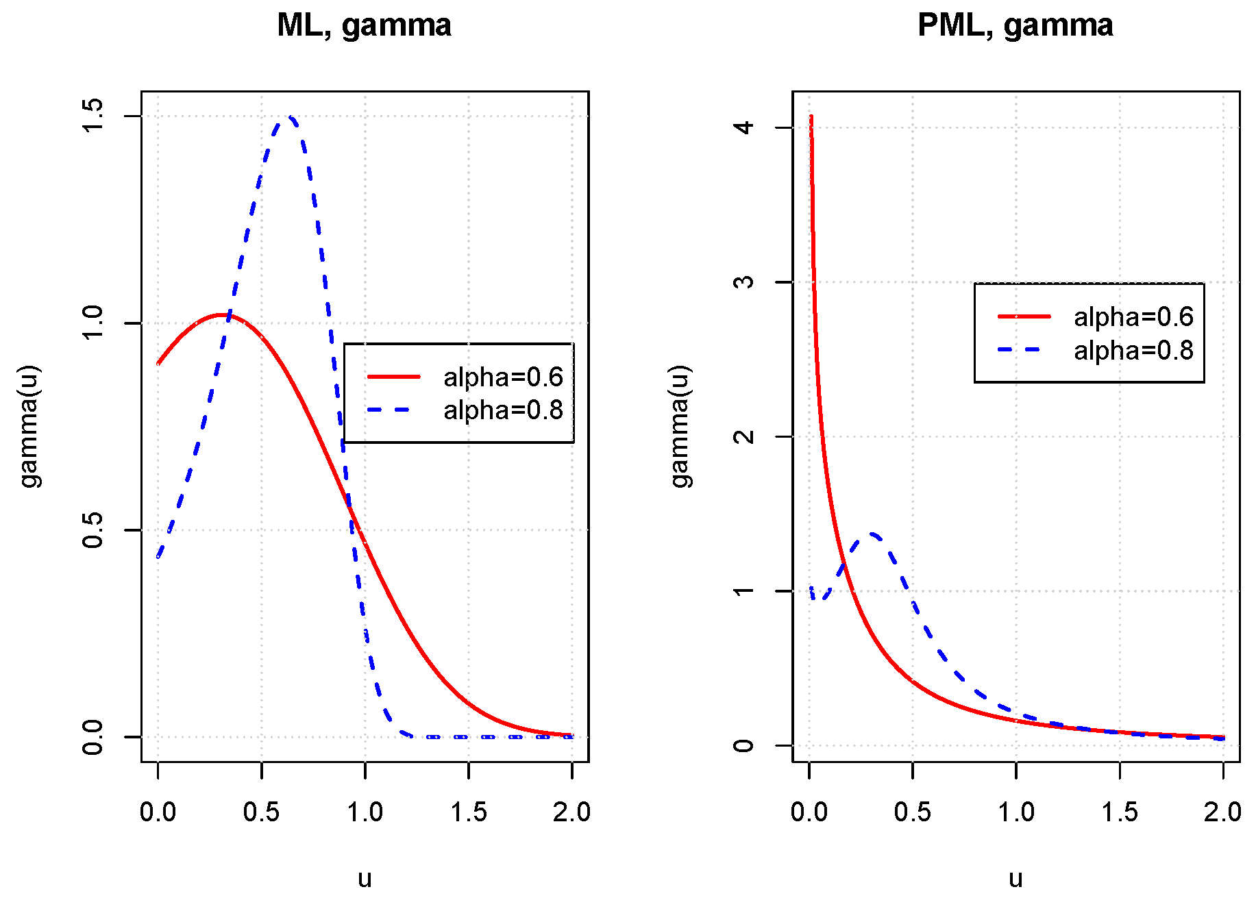
Figure 4 shows the differential of measures $d\gamma (.)$ of the ML and PML kernels. For the ML kernels (left plot), decreasing $\alpha$ clearly makes the right tail of $d\gamma (.)$ larger. The right plot also reveals that the construction of the partition requires a particular care for the PML kernel as we have to integrate numerically measure ${\gamma }_{\alpha ,\beta }^{\left(p\right)}\left(z\right)$ that is not defined for $z=0$. The two next propositions, respectively, present the expressions of integrals needed for calculating the discrete equivalent distributions of ${\gamma }_j(.)$ in the ML and PML cases.

Proposition 4.

For the ML kernel, the discrete probability mass of atoms is given by the following:

$$\begin{array}{ccc}& & m_{k+1}^{\left(j\right)}={\int }_{{\xi }_k^{\left(n\right)}}^{{\xi }_{k+1}^{\left(n\right)}}d{\gamma }_j\left(z\right)\hfill \\ & & =\frac{1}{\pi {\alpha }_j}\sum _{l=1}^{\infty }\frac{{\left(-1\right)}^{l-1}}{l{\beta }_j^{l}l!}sin\left(\pi {\alpha }_{j}l\right)\mathsf{\Gamma }\left({\alpha }_{j}l+1\right)\left[{\left({\xi }_{k+1}^{\left(n\right)}\right)}^l-{\left({\xi }_k^{\left(n\right)}\right)}^l\right],\hfill \end{array}$$

(30)

whereas the numerator in the expression of barycenters (27) is the following.

$$\begin{array}{ccc}\hfill {\int }_{{\xi }_k^{\left(n\right)}}^{{\xi }_{k+1}^{\left(n\right)}}zd{\gamma }_j\left(z\right)& =& \frac{1}{\pi {\alpha }_j}\sum _{l=1}^{\infty }\frac{{\left(-1\right)}^{l-1}}{{\beta }^l(l+1)!}sin\left(\pi {\alpha }_{j}l\right)\mathsf{\Gamma }({\alpha }_{j}l+1)\left[{\left({\xi }_{k+1}^{\left(n\right)}\right)}^{l+1}-{\left({\xi }_k^{\left(n\right)}\right)}^{l+1}\right].\hfill \end{array}$$

(31)

This result is a direct consequence of the definition of the ML function. To the best of our knowledge, these expressions does not admit any other representations. In the PML case, barycenters have a closed-form expression.

Proposition 5.

For the PML kernel, the discrete probability mass of atoms is given by the following.

$$\begin{array}{ccc}\hfill m_{k+1}^{\left(j\right)}={\int }_{{\xi }_k^{\left(n\right)}}^{{\xi }_{k+1}^{\left(n\right)}}d{\gamma }_j\left(z\right)& =& \frac{1}{\pi {\alpha }_j}arctan\left(\frac{{\left({\xi }_{k+1}^{\left(n\right)}\right)}^{{\alpha }_j}+{\beta }_{j}cos\left(\pi {\alpha }_j\right)}{{\beta }_{j}sin\left(\pi {\alpha }_j\right)}\right)\hfill \\ & & -\frac{1}{\pi {\alpha }_j}arctan\left(\frac{{\left({\xi }_k^{\left(n\right)}\right)}^{{\alpha }_j}+{\beta }_{j}cos\left(\pi {\alpha }_j\right)}{{\beta }_{j}sin\left(\pi {\alpha }_j\right)}\right).\hfill \end{array}$$

(32)

The numerator in the expression of barycenters (27) does not admit a closed form expression but may be approached by the following.

$$\begin{array}{ccc}\hfill {\int }_{{\xi }_k^{\left(n\right)}}^{{\xi }_{k+1}^{\left(n\right)}}zd{\gamma }_j\left(z\right)& \approx & \left(\frac{{\xi }_{k+1}^{\left(n\right)}+{\xi }_k^{\left(n\right)}}{2\pi {\alpha }_j}\right)\left[arctan\left(\frac{{\left({\xi }_{k+1}^{\left(n\right)}\right)}^{\alpha }+{\beta }_{j}cos\left(\pi {\alpha }_j\right)}{{\beta }_{j}sin\left(\pi {\alpha }_j\right)}\right)\right.\hfill \\ & & \left.-arctan\left(\frac{{\left({\xi }_k^{\left(n\right)}\right)}^{\alpha }+{\beta }_{j}cos\left(\pi {\alpha }_j\right)}{{\beta }_{j}sin\left(\pi {\alpha }_j\right)}\right)\right].\hfill \end{array}$$

(33)

Proof. 

The expression of the probability mass $m_{k+1}^{\left(j\right)}$ comes from the following relation.

$$\frac{\beta sin\left(\alpha \pi \right)}{\pi }\int \frac{z^{\alpha -1}}{z^{2\alpha }+2\beta z^{\alpha }cos\left(\alpha \pi \right)+{\beta }^2}dz=\frac{1}{\pi \alpha }arctan\left(\frac{z^{\alpha }+\beta cos\left(\pi \alpha \right)}{\beta sin\left(\pi \alpha \right)}\right)$$

The second result is obtained with an integration by parts in which the integral is approached with the trapezoidal method. □

To lighten further developments, we adopt the following notations $Y_s^{(j,k)}:=Y_s^{(j,b_k^{\left(n\right)})}$ for $k=1,\dots ,n$ and $j=1,\dots ,d$. Let us first recall that $Y_0^{(j,k)}=0$ and therefore $Y_s^{(j,k)}$ is an integral from zero to s with respect to the $j\mathrm{th}$ Lévy process.

$$Y_s^{(j,k)}={\int }_0^s{e}^{-b_k^{\left(j\right)}(s-u)}d{L}_u^{\left(j\right)}.$$

(34)

Replacing the continuous measures ${\left({\gamma }_j\right)}_{j=1\dots d}$ by their discrete equivalents results in approximation $r_s^{\left(n\right)}$ of the short-term rate $r_s$.

$$\begin{array}{cc}\hfill r_s^{\left(n\right)}& ={\phi }^{\left(n\right)}\left(s\right)+\sum _{j=1}^d\sum _{k=1}^n{m}_k^{\left(j\right)}{Y}_s^{(j,k)}.\hfill \end{array}$$

(35)

We adopt the following notation $B^{(j,k)}(s,t)=\frac{1}{b_k^{\left(j\right)}}\left(1-e^{-b_k^{\left(j\right)}(t-s)}\right)$ for $k=1,\dots ,n$ and $j=1,\dots ,d$. The bond price in the discretized model with partitions of size n is denoted by $P^{\left(n\right)}(s,t)$ and is equal to the following:

$$\begin{array}{ccc}\hfill P^{\left(n\right)}(s,t)& =& exp\left(-{\int }_s^t{\phi }^{\left(n\right)}\left(u\right)du-\sum _{j=1}^d\sum _{k=1}^n{Y}_s^{(j,k)}{B}^{(j,k)}(s,t)m_k^{\left(j\right)}\right)\hfill \\ & & \times \prod _{j=1}^{d}exp\left({\int }_s^t{\psi }_j\left(-\sum _{k=1}^n{B}^{(j,k)}(v,t)m_k^{\left(j\right)}\right)dv\right),\hfill \end{array}$$

(36)

where ${\phi }^{\left(n\right)}\left(t\right)$ is the discretized version of $\phi \left(t\right)$.

$$\begin{array}{ccc}\hfill {\phi }^{\left(n\right)}\left(t\right)& =& -\frac{\partial }{\partial t}ln\left(P(0,t)\right)-\sum _{j=1}^d{\psi }_j\left(-\sum _{k=1}^n{B}^{(j,k)}(0,t)m_k^{\left(j\right)}\right).\hfill \end{array}$$

(37)

As the number of processes in the discretized model is finite, we can apply Itô’s lemma in order to establish the dynamic of $P^{\left(n\right)}(s,t)$.

Proposition 6.

The zero coupon bond price $P^{\left(n\right)}(s,t)$ is a geometric Lévy processes solution of the SDE:

$$\begin{array}{ccc}& & \frac{d{P}^{\left(n\right)}(s,t)}{P^{\left(n\right)}(s,t)}=r_s^{\left(n\right)}ds-\sum _{j=1}^d{\sigma }_j\sum _{k=1}^n{B}^{(j,k)}(s,t)m_k^{\left(j\right)}d{W}_s^{\left(j\right)}\hfill \\ & & +\sum _{j=1}^d{\int }_{\mathbb{R}}\left(e^{-z\left({\sum }_{k=1}^n{m}_k^{\left(j\right)}{B}^{(j,k)}(s,t)\right)}-1\right)\left(J_j(ds,dz)-{\nu }_j\left(dz\right)ds\right).\hfill \end{array}$$

(38)

with the terminal condition $P^{\left(n\right)}(t,t)=1$.

Proof. 

If we remember that $d{Y}_s^{(j,k)}=d{L}_s^{\left(j\right)}-b_k^{\left(j\right)}{Y}_s^{(j,k)}ds$, the Itô’s lemma provides us with the following differential for $P^{\left(n\right)}(s,t)$.

$$\begin{array}{ccc}& & d{P}^{\left(n\right)}(s,t)=\frac{\partial P^{\left(n\right)}(s,t)}{\partial s}ds-\sum _{j=1}^d\sum _{k=1}^n\frac{\partial P^{\left(n\right)}(s,t)}{\partial Y^{(j,k)}}{b}_k^{\left(j\right)}{Y}_s^{(j,k)}ds\hfill \\ & & +\sum _{j=1}^d\sum _{k=1}^n\frac{\partial P^{\left(n\right)}(s,t)}{\partial Y^{(j,k)}}{\mu }_{j}ds+\sum _{j=1}^d\sum _{k=1}^n\frac{\partial P^{\left(n\right)}(s,t)}{\partial Y^{(j,k)}}{\int }_{\mathbb{R}}z{\tilde{J}}_j(dt,dz)\hfill \\ & & +\sum _{j=1}^d\sum _{k=1}^n\frac{\partial P^{\left(n\right)}(s,t)}{\partial Y^{(j,k)}}{\sigma }_{j}d{W}_s^{\left(j\right)}+\frac{1}{2}\sum _{j=1}^d\sum _{k=1}^n\sum _{l=1}^n\frac{{\partial }^2{P}^{\left(n\right)}(s,t)}{\partial Y^{(j,k)}\partial Y^{(j,l)}}{\sigma }_j^{2}ds\hfill \\ & & +\sum _{j=1}^d{\int }_{\mathbb{R}}{P}^{\left(n\right)}(s,t)\left(e^{-z\left({\sum }_{k=1}^n{m}_k^{\left(j\right)}{B}^{(j,k)}(s,t)\right)}-1\right)-z\sum _{k=1}^n\frac{\partial P^{\left(n\right)}(s,t)}{\partial Y^{(j,k)}}{J}_j(ds,dz).\hfill \end{array}$$

(39)

The first and second order partial derivatives of $P^{\left(n\right)}(s,t)$ are equal to the following.

$$\frac{\partial P^{\left(n\right)}(s,t)}{\partial Y^{(j,k)}}=-P^{\left(n\right)}(s,t)B^{(j,k)}(s,t)m_k^{\left(j\right)},$$

(40)

$$\begin{array}{cc}\hfill \frac{{\partial }^2{P}^{\left(n\right)}(s,t)}{\partial Y^{(j,k)}\partial Y^{(i,l)}}& =P^{\left(n\right)}(s,t)B^{(j,k)}(s,t)B^{(i,l)}(s,t)m_k^{\left(j\right)}{m}_l^{\left(i\right)}.\hfill \end{array}$$

(41)

On the other hand, its partial derivative with respect to time is given by the following:

$$\begin{array}{ccc}\hfill \frac{\partial P^{\left(n\right)}(s,t)}{\partial s}& =& P^{\left(n\right)}(s,t)\left({\phi }^{\left(n\right)}\left(s\right)+\sum _{j=1}^d\sum _{k=1}^n{Y}_s^{(j,k)}{e}^{-b_k^{\left(j\right)}(t-s)}{m}_k^{\left(j\right)}\right.\hfill \\ & & \left.-\sum _{j=1}^d{\psi }_j\left(-\sum _{k=1}^n{B}^{(j,k)}(s,t)m_k^{\left(j\right)}\right)\right),\hfill \end{array}$$

(42)

where the characteristic exponent is developed as the following sum.

$$\begin{array}{cc}\hfill & {\psi }_j\left(-\sum _{k=1}^n{B}^{(j,k)}(s,t)m_k^{\left(j\right)}\right)=-{\mu }_j\sum _{k=1}^n{B}^{(j,k)}(s,t)m_k^{\left(j\right)}+\frac{1}{2}{\left(\sum _{k=1}^n{B}^{(j,k)}(s,t)m_k^{\left(j\right)}\right)}^2{\sigma }_j^2\hfill \\ \hfill & {\int }_{\mathbb{R}}\left(e^{-\left({\sum }_{k=1}^n{B}^{(j,k)}(s,t)m_k^{\left(j\right)}\right)z}-1+\left(\sum _{k=1}^n{B}^{(j,k)}(s,t)m_k^{\left(j\right)}\right)z{1}_{\left|z\right|<ϵ}\right){\nu }_j\left(dz\right).\hfill \end{array}$$

(43)

Combining Equations (39)–(43) allows us to rewrite the dynamic of bond prices as follows.

$$\begin{array}{ccc}& & d{P}^{\left(n\right)}(s,t)=P^{\left(n\right)}(s,t)\left({\phi }^{\left(n\right)}\left(s\right)+\sum _{j=1}^d\sum _{k=1}^n{Y}_s^{(j,k)}{e}^{-b_k^{\left(j\right)}(t-s)}{m}_k^{\left(j\right)}\right)ds\hfill \\ & & +P^{\left(n\right)}(s,t)\sum _{j=1}^d\sum _{k=1}^n{Y}_s^{(j,k)}{B}^{(j,k)}(s,t)m_k^{\left(j\right)}{b}_k^{\left(j\right)}ds\hfill \\ & & -P^{\left(n\right)}(s,t)\sum _{j=1}^d{\sigma }_j\sum _{k=1}^n{B}^{\left(k\right)}(s,t)m_k^{\left(n\right)}d{W}_s^{\left(j\right)}\hfill \\ & & +P^{\left(n\right)}(s,t)\sum _{j=1}^d{\int }_{\mathbb{R}}\left(e^{-z\left({\sum }_{k=1}^n{m}_k^{\left(j\right)}{B}^{(j,k)}(s,t)\right)}-1\right)\left(J_j(ds,dz)-{\nu }_j\left(dz\right)ds\right).\hfill \end{array}$$

We infer the result if we remember Equation (35) and notice that the following is the case.

$$\begin{array}{cc}\hfill \sum _{k=1}^n{Y}_s^{(j,k)}{e}^{-b_k^{\left(j\right)}(t-s)}{m}_k^{\left(j\right)}+\sum _{k=1}^n{Y}_s^{(j,k)}{B}^{\left(k\right)}(s,t)m_k^{\left(j\right)}{b}_k^{\left(j\right)}& =\sum _{k=1}^n{Y}_s^{(j,k)}{m}_k^{\left(j\right)}.\hfill \end{array}$$

□

As by construction ${lim}_{n\to \infty }{\gamma }_j^{\left(n\right)}\left(z\right)={\gamma }_j\left(z\right)$, we immediately infer the dynamic of the bond price in the non-discretized model by considering the limit of Equation (38).

Corollary 1.

If the short-term rate is driven by Equation (19), the bond price is solution of the following SDE:

$$\begin{array}{ccc}& & \frac{dP(s,t)}{P(s,t)}=r_{s}ds-\sum _{j=1}^d{\sigma }_j{h}_j(s,t)d{W}_s^{\left(j\right)}\hfill \\ & & +\sum _{j=1}^d{\int }_{\mathbb{R}}\left(e^{-z{h}_j(s,t)}-1\right)\left(J_j(ds,dz)-{\nu }_j\left(dz\right)ds\right).\hfill \end{array}$$

(44)

where $h_j(s,t)={\int }_0^{\infty }{B}^{\left(\xi \right)}(s,t)d{\gamma }_j\left(\xi \right)$ and with the terminal condition $P(t,t)=1$.

In order to understand the role played by the memory kernel in the evolution of the term structure of interest rates, we analyze the expectation and variance of bond yields. The bond yield of a zero-coupon bond in the discretized model is defined as follows.

$$y^{\left(n\right)}(s,t)=-\frac{ln{P}^{\left(n\right)}(s,t)}{t-s}.$$

From Equation (36), we infer that this yield is proportional to a weighted sum of mean reverting processes $Y_s^{(j,k)}$. Since $\mathbb{E}\left(Y_s^{(j,k)}|{\mathcal{F}}_0\right)=0$ by construction, the expected yield conditionally to the initial filtration is equal to the following.

$$\begin{array}{cc}\hfill \mathbb{E}\left(y^{\left(n\right)}(s,t)|{\mathcal{F}}_0\right)& =\frac{1}{t-s}\left({\int }_s^t{\phi }^{\left(n\right)}\left(u\right)du-\sum _{j=1}^d{\int }_s^t{\psi }_j\left(-\sum _{k=1}^n{B}^{(j,k)}(v,t)m_k^{\left(j\right)}\right)dv\right).\hfill \end{array}$$

(45)

The variance of the yield is the sum of d variances of a linear combination of processes $Y_s^{(j,k)}$. If we remember that the covariance $Y_s^{(j,k)}$ and $Y_s^{(l,k)}$ is equal to the following:

$$\begin{array}{cc}\hfill \mathbb{C}\left(Y_s^{(j,k)}{Y}_s^{(j,l)}|{\mathcal{F}}_0\right)& =\left({\sigma }_j^2+{\int }_{\mathbb{R}}{z}^2{\nu }_j\left(dz\right)\right){\int }_0^s{e}^{-\left(b_k^{\left(j\right)}+b_l^{\left(j\right)}\right)(s-u)}du\hfill \\ \hfill & =\frac{{\sigma }_j^2+{\int }_{\mathbb{R}}{z}^2{\nu }_j\left(dz\right)}{b_k^{\left(j\right)}+b_l^{\left(j\right)}}\left(1-e^{-\left(b_k^{\left(j\right)}+b_l^{\left(j\right)}\right)s}\right),\hfill \end{array}$$

(46)

the variance of the yield, conditionally to ${\mathcal{F}}_0$, is the following triple sum.

$$\begin{array}{cc}\hfill & \mathbb{V}\left(y^{\left(n\right)}(s,t)|{\mathcal{F}}_0\right)=\sum _{j=1}^d\mathbb{V}\left(\sum _{k=1}^n\frac{B^{(j,k)}(s,t)m_k^{\left(j\right)}}{t-s}{Y}_s^{(j,k)}|{\mathcal{F}}_0\right)\hfill \\ \hfill & =\sum _{j=1}^d\left[\sum _{k=1}^n\sum _{l=1}^n\frac{B^{(j,k)}(s,t)m_k^{\left(j\right)}}{t-s}\frac{B^{(j,l)}(s,t)m_l^{\left(j\right)}}{t-s}\mathbb{C}\left(Y_s^{(j,k)}{Y}_s^{(j,l)}|{\mathcal{F}}_0\right)\right].\hfill \end{array}$$

(47)

To illustrate these results, we consider an univariate jump-diffusion model ($d=1$) in which a single Lévy process is ruled by the following SDE.

$$\begin{array}{ccc}\hfill d{L}_t^{\left(1\right)}& =& -{\lambda }_1{\eta }_{1}dt+{\sigma }_{1}d{W}_t^{\left(1\right)}+{\eta }_{1}d{N}_t^{\left(1\right)}.\hfill \end{array}$$

(48)

$N_t^{\left(1\right)}$ is a Poisson process with constant intensity ${\lambda }_1$. The characteristic exponent is in this case equal to the following:

$$\begin{array}{ccc}\hfill {\psi }_1\left(\omega \right)& =& -{\lambda }_1{\eta }_1\omega +\frac{1}{2}{\omega }^2{\sigma }_1^2+{\lambda }_1\left(e^{\omega {\eta }_1}-1\right),\hfill \end{array}$$

(49)

whereas the Lévy measure is ${\nu }_1\left(z\right)={\lambda }_1{\delta }_{{\eta }_1}\left(z\right)$ where ${\delta }_{{\eta }_1}\left(z\right)$ is the Dirac measure located at $z={\eta }_1$. The instantaneous variance of $d{L}_t^{\left(1\right)}$ is equal to the following.

$$\begin{array}{ccc}\hfill {\sigma }_1^2+{\int }_{\mathbb{R}}{z}^2{\nu }_1\left(dz\right)& =& {\sigma }_1^2+{\lambda }_1{\eta }_1^2.\hfill \end{array}$$

Of course, we can consider other types of Lévy processes such as the variance gamma and the Normal inverse gaussian, but this does not fundamentally modify the conclusions drawn in this section. We first fit the curve $\phi \left(t\right)$ to the term structure of zero-coupon bond yields, bootstrapped from the ICE swap rates on the 26/2/21 at noon. Since this function is proportional to instantaneous forward rates, we have to interpolate bond yields. For this purpose, we use a Nelson–Siegel (NS) model. Appendix B recalls this model and reports the swap rates curve on the 26/2/21 and parameter estimates. There exist more advanced interpolation methods such as, e.g., splines or kriging techniques as detailed in Cousin et al. (2016) but the NS model is sufficiently accurate for our purposes to understand the dynamic of yields over time.

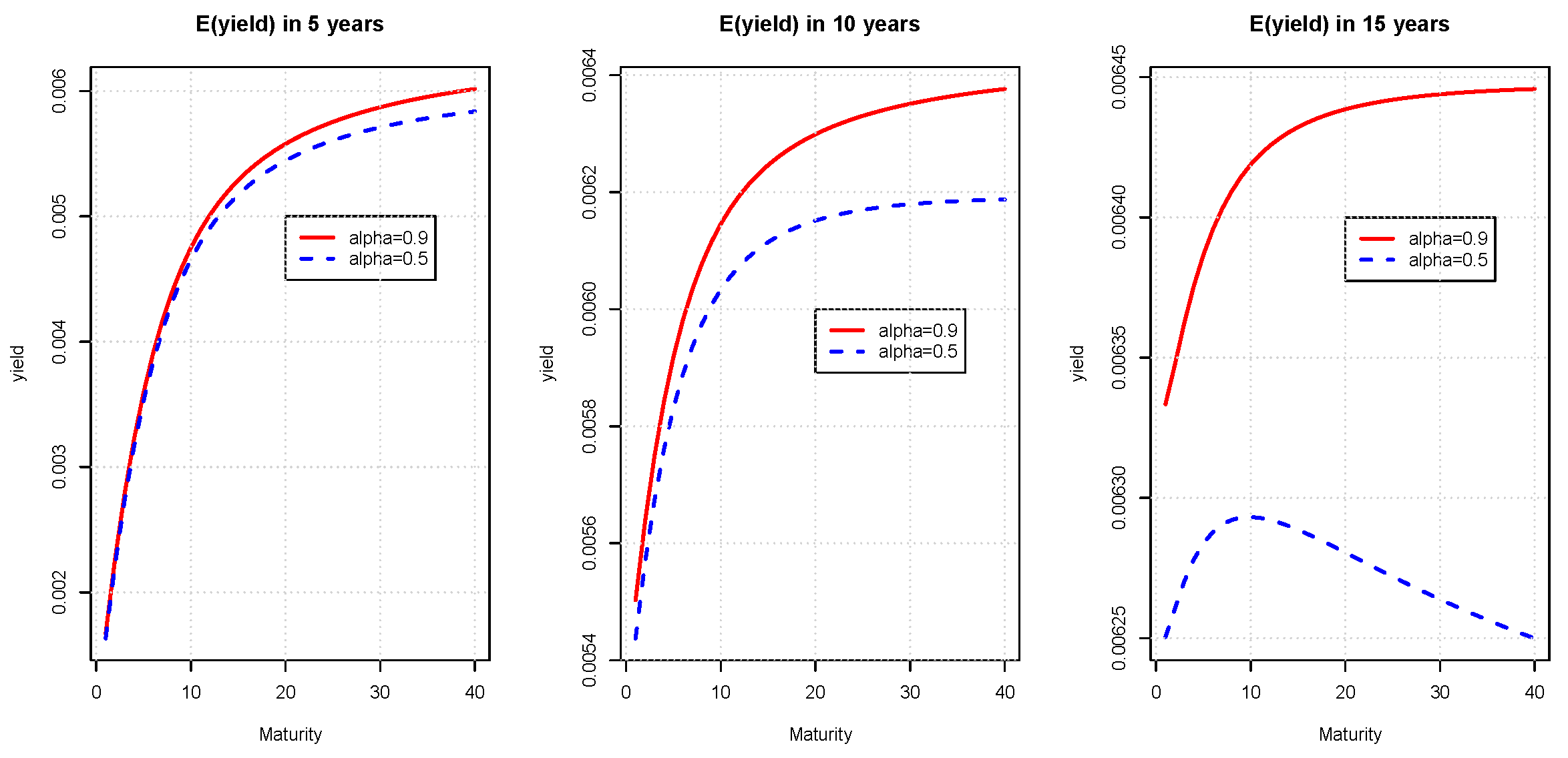
We calculate the term structure of expected yields in 5, 10 and 15 years with $n=$ 40 atoms. Increasing n does not significantly modify the results. A sensitivity analysis with respect to the number of atoms is proposed in Section 7. For the parameters, we set $\beta =1.5$, ${\lambda }_1=0.5$, ${\sigma }_1=0.01$ and ${\eta }_1=-0.0002$, which are possible realistic values in view of results from Section 3. We remind the reader that $\alpha$ is the parameter tuning the memory of the model. If $\alpha =1$, the memory kernel is exponential and the model forgets in an exponential manner past fluctuations of interest rates. On the other hand, for lower values of $\alpha$, the model forgets these variations according to a power decaying function. Figure 5 and Figure 6 show expected yields computed with the ML and PML models for $\alpha =0.5$ and $\alpha =0.9$. We use a discretization scheme with 40 atoms that cover ML and PML density up to their 90% percentiles. For both models, the range between short and long-term yields is narrowing with the time horizon. In the ML model, the lower $\alpha$ is, the longer the memory and the quicker the convergence to a bumped (but nearly flat) yield curve. In the PML model, expected yield curves with a low $\alpha$ dominate those with a high $\alpha$ and have a more pronounced curvature.

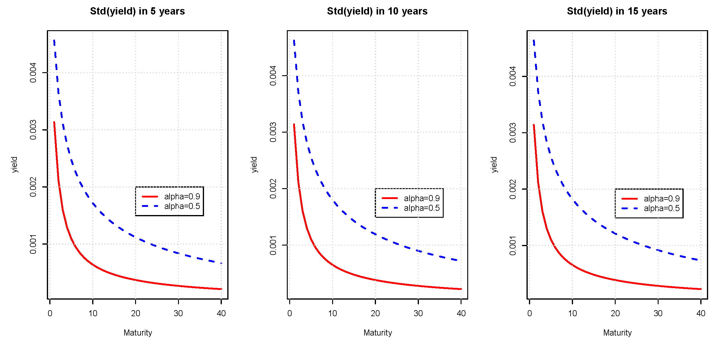
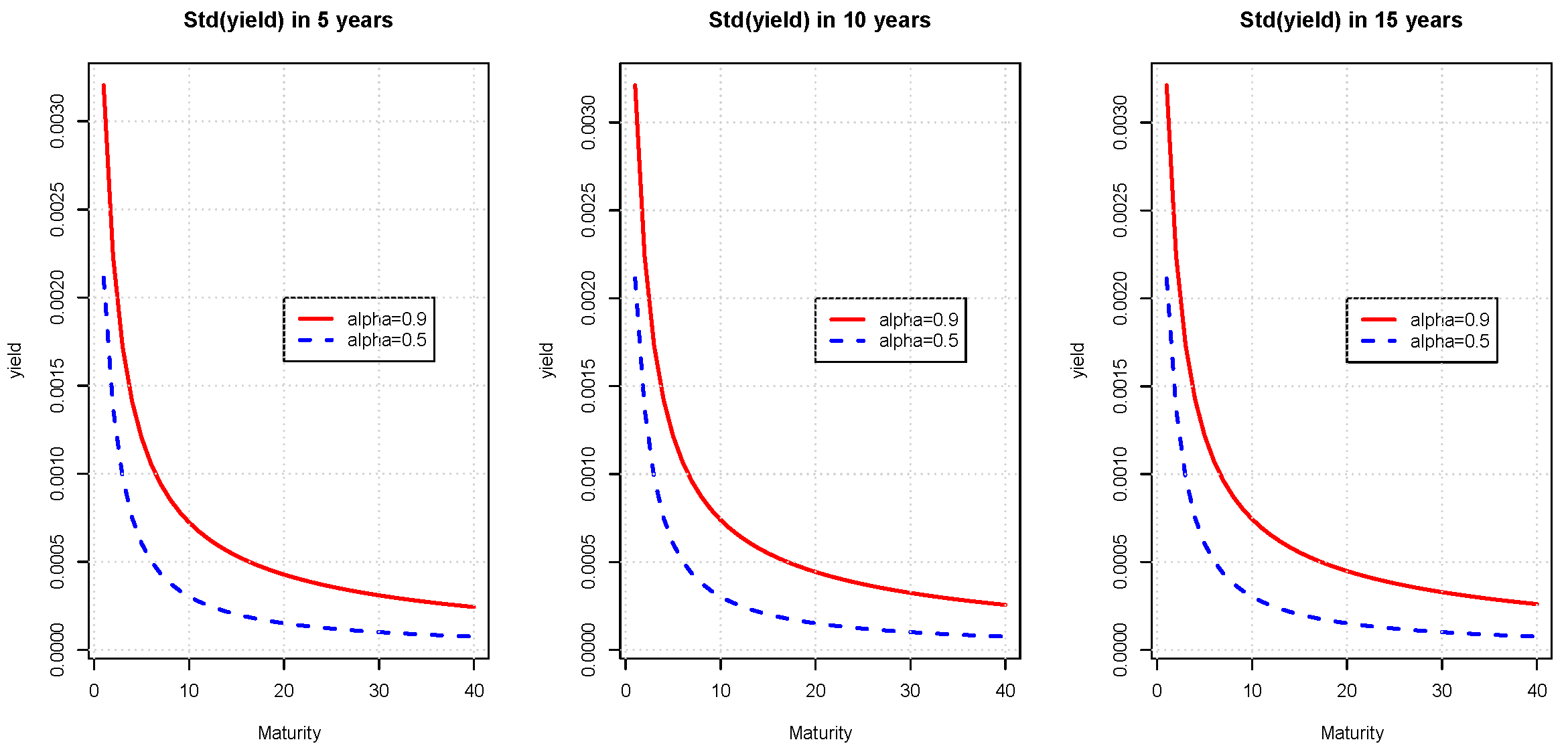
Figure 7 and Figure 8 report the expected standard deviations of future yields calculated with ML and PML models. In both cases, the term structures of expected standard deviations do not significantly evolve with the time horizon and are decreasing functions of the maturity. We also notice that standard deviations are, respectively, inversely and directly proportional to $\alpha$ in ML and PML models.

7. Pricing of Bond Options

The purpose of this section is to illustrate how long-term memory models can be used for the pricing of derivatives. We investigate this for European options written on a zero coupon bond. Our choice is motivated by the fact that these are the building blocks of many structured products. The underlying bond has a maturity noted $t_2$ while the option expires at time $t_1\le t_2$ with a strike price K. Without loss of generality we focus on a call option but all developments remain valid for any other type of European options. The value at time $s\le t_1\le t_2$ of the call option is denoted by $C\left(s\right)$ and is equal to the expected discounted payoff under the risk neutral measure $\mathbb{Q}$.

$$\begin{array}{ccc}\hfill C\left(s\right)& =& \mathbb{E}\left(e^{-{\int }_s^{t_1}{r}_{u}du}{\left(P(t_1,t_2)-K\right)}_{+}|{\mathcal{F}}_s\right).\hfill \end{array}$$

This price does not admit any closed form expression. Nevertheless, we can apply the standard technique of changes of numeraire combined with a discrete Fourier’s transform (DFT) to evaluate this call option. The first stage consists to define a forward measure, denoted by $\mathbb{F}$ that has $P(s,t_1)$ as numeraire, i.e., every assets discounted by $P(s,t_1)$ is a martingale. If $S_t^{\left(0\right)}=e^{{\int }_0^t{r}_{u}du}$ is the cash account (numeraire of $\mathbb{Q}$), the Radon–Nykodym derivative defining this change of measure is ${\left.\frac{d\mathbb{F}}{d\mathbb{Q}}\right|}_{t_1}=\frac{S_0^{\left(0\right)}}{S_{t_1}^{\left(0\right)}P(0,t_1)}$. Using standard arguments, the call price is equal to the product of a discount bond and of the expected payoff under this forward measure.

$$\begin{array}{ccc}\hfill C\left(s\right)& =& P(s,t_1){\mathbb{E}}^{\mathbb{F}}\left({\left(P(t_1,t_2)-K\right)}_{+}|{\mathcal{F}}_s\right).\hfill \end{array}$$

(50)

The next proposition details the dynamics of underlying Lévy processes under the forward measure.

Proposition 7.

Under the forward measure $\mathbb{F}$ with $P(s,t_1)$ as numeraire, the process ${\left(W_s^{\left(j\right)\mathbb{F}}\right)}_{s\ge 0}$ is the following:

$$d{W}_s^{\left(j\right)\mathbb{F}}=d{W}_t^{\left(j\right)}+h_j(u,t_1)du.$$

(51)

for $j=1,\dots d$ is a Brownian motion. Furthermore, the random measure is the following:

$$\begin{array}{ccc}\hfill {\tilde{J}}_j^{\mathbb{F}}(du,dz)& =& {\tilde{J}}_j(du,dz)-1_{\left|z\right|<ϵ}\left(e^{-h_j(u,t_1)z}-1\right){\nu }_j\left(dz\right)du,\hfill \end{array}$$

(52)

for $j=1,\dots d$ defines a jump process under $\tilde{\mathbb{P}}$ with the time-varying measure ${\nu }_j^{\mathbb{F}}(dt,dz)=e^{-h_j(u,t_1)z}{\nu }_j\left(dz\right)$.

Proof. 

From Applebaum (2004, chap. 5, secs. 2 and 4), the forward change of the following measure:

$$\begin{array}{cc}\hfill {\left.\frac{d\mathbb{F}}{d\mathbb{Q}}\right|}_{t_1}& =\frac{S_0^{\left(0\right)}}{S_{t_1}^{\left(0\right)}P(0,t_1)}\hfill \\ \hfill & =exp\left(\sum _{j=1}^d{\int }_0^{t_1}-h_j(u,t_1){\sigma }_{j}d{W}_u^{\left(j\right)}-\frac{1}{2}{h}_j{(u,t_1)}^2{\sigma }_j^{2}du\right.\hfill \\ \hfill & -\sum _{j=1}^d{\int }_0^{t_1}{\int }_{\mathbb{R}}\left(e^{-h_j(u,t_1)z}-1+h_j(u,t_1)z{1}_{\left|z\right|<ϵ}\right){\nu }_j\left(dz\right)du\hfill \\ \hfill & \left.+\sum _{j=1}^d{\int }_0^{t_1}{\int }_{\left|z\right|\ge ϵ}-h_j(u,t_1)z{\tilde{J}}_j(du,dz)\right)\hfill \end{array}$$

(53)

is a martingale under the measure $\mathbb{Q}$, which defines an equivalent measure $\mathbb{F}$ under which ${\left(W_s^{\left(j\right)\mathbb{F}}\right)}_{s\ge 0}$ and ${\tilde{J}}_j^{\mathbb{F}}(du,dz)$ for $j=1,\dots d$ are, respectively, Brownian motions and random jump measures satisfying Equations (51) and (52). □

Combining Corollary 1 and Proposition 7 allows us to infer that a zero-coupon bond of maturity $t\ge t_1$ is ruled under the forward measure by the SDE.

$$\begin{array}{ccc}\hfill \frac{dP(s,t)}{P(s,t)}& =& \left(r_s+\sum _{j=1}^d{\sigma }_j{h}_j{(s,t_1)}^2+\sum _{j=1}^d{\int }_{\mathbb{R}}{\left(e^{-z{h}_j(s,t_1)}-1\right)}^2{\nu }_j\left(dz\right)\right)ds\hfill \\ & & +\sum _{j=1}^d{\int }_{\mathbb{R}}\left(e^{-z{h}_j(s,t_1)}-1\right)\left(J_j^{\mathbb{F}}(ds,dz)-e^{-h_j(s,t_1)z}{\nu }_j\left(dz\right)ds\right)\hfill \\ & & -\sum _{j=1}^d{\sigma }_j{h}_j(s,t_1)d{W}_s^{\left(j\right)\mathbb{F}}.\hfill \end{array}$$

(54)

This equation emphasizes that the average bond return under the forward measure is the risk-free rate plus a positive time varying premium that converges toward zero when $s\to t_1$. The next proposition reveals that the processes $Y_t^{(j,\xi )}$ do not revert anymore toward zero under $\mathbb{F}$.

Proposition 8.

Let us define the following function.

$$\begin{array}{cc}\hfill {\theta }^{(j,\xi )}\left(u\right)& =\left\{\begin{array}{cc}-\left(h_j(u,t_1){\sigma }_j+{\int }_{\mathbb{R}}z\left(1-e^{-h_j(u,t_1)z}{1}_{\left|z\right|<ϵ}\right){\nu }_j\left(dz\right)\right)\hfill & \xi >0\hfill \\ 0\hfill & \xi =0\hfill \end{array}\right..\hfill \end{array}$$

(55)

Under the forward measure $\mathbb{F}$, $Y_t^{(j,\xi )}$ is a process reverting to ${\theta }^{(j,\xi )}\left(t\right)/\xi$ at a speed ξ such that the following is the case:

$$\begin{array}{cc}\hfill Y_t^{(j,\xi )}& =e^{-\xi (t-s)}{Y}_s^{\left(j\right)}+{\int }_s^t{e}^{-\xi (t-u)}{\theta }^{(j,\xi )}\left(u\right)du\hfill \\ \hfill & +{\sigma }_j{\int }_s^t{e}^{-\xi (t-u)}d{W}_u^{\left(j\right)\mathbb{F}}+{\int }_s^t{e}^{-\xi (t-u)}{\int }_{\mathbb{R}}z{\tilde{J}}_j^{\mathbb{F}}(du,dz),\hfill \end{array}$$

(56)

for all $j=1,\dots ,d$ and $\xi \in {\mathbb{R}}^{+}$.

Proof. 

By definition of $Y_s^{(j,\xi )}$ and from Corollary 1, we immediately infer its dynamic under the forward measure.

$$\begin{array}{cc}\hfill d{Y}_s^{(j,\xi )}& =-\xi Y_s^{(j,\xi )}ds+{\sigma }_{j}d{W}_s^{\left(j\right)\mathbb{F}}+{\int }_{\mathbb{R}}z{\tilde{J}}_j^{\mathbb{F}}(ds,dz)\hfill \\ \hfill & +\left({\mu }_j-h_j(s,t_1){\sigma }_j+{\int }_{\left|z\right|<ϵ}z\left(e^{-h_j(s,t_1)z}-1\right){\nu }_j\left(dz\right)\right)ds.\hfill \end{array}$$

(57)

Since we impose that ${\mu }_j=-{\int }_{\mathbb{R}}\left(z-z{1}_{\left|z\right|<ϵ}\right){\nu }_j\left(dz\right)$ for $j=1,\dots ,d$ in order to ensure that $\mathbb{E}\left(L_t^{\left(j\right)}\right)=0$, we deduce that $Y_s^{(j,\xi )}$ reverts to ${\theta }^{(j,\xi )}\left(t\right)/\xi$:

$$\begin{array}{ccc}\hfill d{Y}_s^{(j,\xi )}& =& \xi \left(\frac{1}{\xi }{\theta }^{(j,\xi )}\left(s\right)-Y_s^{(j,\xi )}\right)ds+{\sigma }_{j}d{W}_s^{\left(j\right)\mathbb{F}}+{\int }_{\mathbb{R}}z{\tilde{J}}_j^{\mathbb{F}}(ds,dz),\hfill \end{array}$$

and the solution of this SDE is Equation (56). □

Equations (53) and (57) are useful for simulating sample paths of interest rates and bond prices under the forward measure, e.g., for pricing exotic options. One solution to price a call option on a zero-coupon bond consists in numerically inverting the Fourier’s transform of the density of its bond log-return under the forward measure. This step is performed with a standard discrete Fourier’s transform algorithm (DFT) that approximates the probability density function of the log-return under the forward measure $\mathbb{F}$. The expectation of the payoff under the forward measure is next computed with this distribution. The moment generating function of the bond log-return, presented in the next proposition, admits a closed form formula and is a key result to implementing the DFT procedure.

Proposition 9.

The moment generating function (mgf) of $lnP(t_1,t_2)$ under measure $\mathbb{F}$, conditionally to the filtration ${\mathcal{F}}_s$, is given by the following.

$$\begin{array}{ccc}& & {\mathbb{E}}^{\mathbb{F}}\left(e^{\omega lnP(t_1,t_2)}|{\mathcal{F}}_s\right)=\hfill \\ & & exp\left(-\sum _{j=1}^d{\int }_s^{t_1}{\psi }_j\left(-h_j(u,t_1)\right)du-\omega {\int }_{t_1}^{t_2}\phi \left(u\right)du+\omega \sum _{j=1}^d{\int }_{t_1}^{t_2}{\psi }_j\left(-h_j(u,t_2)\right)du\right)\hfill \\ & & \times exp\left(-\omega \sum _{j=1}^d{\int }_0^{\infty }{Y}_s^{(j,\xi )}{e}^{-\xi (t_1-s)}{B}^{\left(\xi \right)}(t_1,t_2)d{\gamma }_j\left(\xi \right)\right)\hfill \\ & & exp\left(\sum _{j=1}^d{\int }_s^{t_1}{\psi }_j\left(-{\int }_0^{\infty }\frac{1}{\xi }\left(1-\left(1+\omega \right)e^{-\xi (t_1-u)}+\omega e^{-\xi (t_2-u)}\right)d{\gamma }_j\left(\xi \right)\right)du\right).\hfill \end{array}$$

(58)

Proof. 

The mgf can be rewritten as an expectation under the risk neutral measure using Bayes’ rule:

$$\begin{array}{ccc}\hfill {\mathbb{E}}^{\mathbb{F}}\left(e^{\omega lnP(t_1,t_2)}|{\mathcal{F}}_s\right)& =& \frac{\mathbb{E}\left({\left.\frac{d\mathbb{F}}{d\mathbb{Q}}\right|}_{t_1}{e}^{\omega lnP(t_1,t_2)}|{\mathcal{F}}_s\right)}{\mathbb{E}\left({\left.\frac{d\mathbb{F}}{d\mathbb{Q}}\right|}_{t_1}|{\mathcal{F}}_s\right)},\hfill \end{array}$$

(59)

where ${\left.\frac{d\mathbb{F}}{d\mathbb{Q}}\right|}_{t_1}$ is detailed in Equation (53). From Equation (24) and due to the independence between the processes $Y_{t_1}^{(j,\xi )}$ and $Y_{t_1}^{(k,\xi )}$ for $j\ne k$, expectation (59) becomes the following.

$$\begin{array}{ccc}& & {\mathbb{E}}^{\mathbb{F}}\left(e^{\omega lnP(t_1,t_2)}|{\mathcal{F}}_s\right)=\hfill \\ & & exp\left(-\sum _{j=1}^d{\int }_s^{t_1}{\psi }_j\left(-h_j(u,t_1)\right)du-\omega {\int }_{t_1}^{t_2}\phi \left(u\right)du+\omega \sum _{j=1}^d{\int }_{t_1}^{t_2}{\psi }_j\left(-h_j(u,t_2)\right)du\right)\hfill \\ & & \times \prod _{j=1}^d\mathbb{E}\left(exp\left(-{\int }_s^{t_1}{h}_j(u,t_1)d{L}_u^{\left(j\right)}-\omega {\int }_0^{\infty }{Y}_{t_1}^{(j,\xi )}{B}^{\left(\xi \right)}(t_1,t_2)d{\gamma }_j\left(\xi \right)\right)|{\mathcal{F}}_s\right).\hfill \end{array}$$

From Equation (18) and after a change of integration order, the integral of processes $Y_{t_1}^{(j,\xi )}$ is the following.

$$\begin{array}{cc}\hfill & {\int }_0^{\infty }{Y}_{t_1}^{(j,\xi )}{B}^{\left(\xi \right)}(t_1,t_2)d{\gamma }_j\left(\xi \right)\hfill \\ \hfill & ={\int }_0^{\infty }{Y}_s^{(j,\xi )}{e}^{-\xi (t_1-s)}{B}^{\left(\xi \right)}(t_1,t_2)d{\gamma }_j\left(\xi \right)+{\int }_0^{\infty }{\int }_s^{t_1}{e}^{-\xi (t_1-u)}d{L}_u^{\left(j\right)}{B}^{\left(\xi \right)}(t_1,t_2)d{\gamma }_j\left(\xi \right)\hfill \\ \hfill & ={\int }_0^{\infty }{Y}_s^{(j,\xi )}{e}^{-\xi (t_1-s)}{B}^{\left(\xi \right)}(t_1,t_2)d{\gamma }_j\left(\xi \right)+{\int }_s^{t_1}{\int }_0^{\infty }{e}^{-\xi (t_1-u)}{B}^{\left(\xi \right)}(t_1,t_2)d{\gamma }_j\left(\xi \right)d{L}_u^{\left(j\right)}.\hfill \end{array}$$

This allows us to rewrite ${\mathbb{E}}^{\mathbb{F}}\left(e^{\omega lnP(t_1,t_2)}|{\mathcal{F}}_s\right)$ as follows,

$$\begin{array}{ccc}& & {\mathbb{E}}^{\mathbb{F}}\left(e^{\omega lnP(t_1,t_2)}|{\mathcal{F}}_s\right)=\hfill \\ & & exp\left(-\sum _{j=1}^d{\int }_s^{t_1}{\psi }_j\left(-h_j(u,t_1)\right)du-\omega {\int }_{t_1}^{t_2}\phi \left(u\right)du+\omega \sum _{j=1}^d{\int }_{t_1}^{t_2}{\psi }_j\left(-h_j(u,t_2)\right)du\right)\hfill \\ & & \times exp\left(-\omega \sum _{j=1}^d{\int }_0^{\infty }{Y}_s^{(j,\xi )}{e}^{-\xi (t_1-s)}{B}^{\left(\xi \right)}(t_1,t_2)d{\gamma }_j\left(\xi \right)\right)\hfill \\ & & \times \prod _{j=1}^d\mathbb{E}\left(exp\left(-{\int }_s^{t_1}\left(h_j(u,t_1)-\omega {\int }_0^{\infty }{e}^{-\xi (t_1-u)}{B}^{\left(\xi \right)}(t_1,t_2)d{\gamma }_j\left(\xi \right)\right)d{L}_u^{\left(j\right)}\right)|{\mathcal{F}}_s\right).\hfill \end{array}$$

By definition of $h_j(u,t):={\int }_0^{\infty }{B}^{\left(\xi \right)}(u,t)d{\gamma }_j\left(\xi \right)$, we have the following:

$$\begin{array}{cc}\hfill & h_j(u,t_1)-\omega {\int }_0^{\infty }{e}^{-\xi (t_1-u)}{B}^{\left(\xi \right)}(t_1,t_2)d{\gamma }_j\left(\xi \right)=\hfill \\ \hfill & \hfill {\int }_0^{\infty }\left(B^{\left(\xi \right)}(u,t_1)-\omega e^{-\xi (t_1-u)}{B}^{\left(\xi \right)}(t_1,t_2)\right)d{\gamma }_j\left(\xi \right),\end{array}$$

wherein the integrand is equal to the following.

$$\begin{array}{ccc}& & B^{\left(\xi \right)}(u,t_1)-\omega e^{-\xi (t_1-u)}{B}^{\left(\xi \right)}(t_1,t_2)\hfill \\ & & =\frac{1}{\xi }\left(1-\left(1+\omega \right)e^{-\xi (t_1-u)}+\omega e^{-\xi (t_2-u)}\right).\hfill \end{array}$$

Combining these three last equations leads to the result. □

The expression (58) of the mgf involves integrals of $Y_s^{(j,\xi )}$ with respect to $\xi \in {\mathbb{R}}^{+}$. These integrals do not admit analytical formulas and are in practice approached with the discretization scheme introduced in Section 6. Let n be the number of atoms of the discrete approximation of ${\gamma }_j$ for $j=1,\dots ,d$. To lighten future developments, we adopt the following notation:

$$\begin{array}{ccc}\hfill h_j^{\left(n\right)}(u,t)& :=& \sum _{k=1}^n\frac{m_k^{\left(j\right)}}{b_k^{\left(j\right)}}\left(1-e^{-b_k^{\left(j\right)}(t-u)}\right),\hfill \\ \hfill g_j^{\left(n\right)}(\omega ,u,t_1,t_2)& :=& \sum _{k=1}^n\frac{m_k^{\left(j\right)}}{b_k^{\left(j\right)}}\left(1-\left(1+\omega \right)e^{-b_k^{\left(j\right)}(t_1-u)}+\omega e^{-b_k^{\left(j\right)}(t_2-u)}\right),\hfill \end{array}$$

for $j=1,\dots ,d$. The discretized version of the mgf of the bond log-return under the forward measure is as follows:

$$\begin{array}{ccc}& & {\mathbb{E}}^{\mathbb{F}}\left(e^{\omega ln{P}^{\left(n\right)}(t_1,t_2)}|{\mathcal{F}}_s\right)=\hfill \\ & & exp\left(\sum _{j=1}^d{\int }_s^{t_1}{\psi }_j\left(-g_j^{\left(n\right)}(\omega ,u,t_1,t_2)\right)-{\psi }_j\left(-h_j^{\left(n\right)}(u,t_1)\right)du\right)\hfill \\ & & \times exp\left({\int }_{t_1}^{t_2}\omega \sum _{j=1}^d{\psi }_j\left(-h_j^{\left(n\right)}(u,t_2)\right)-\omega {\phi }^{\left(n\right)}\left(u\right)du\right)\hfill \\ & & \times exp\left(-\sum _{j=1}^d\sum _{k=1}^n{m}_k^{\left(j\right)}{Y}_s^{(j,k)}{e}^{-b_k^{\left(j\right)}(t_1-s)}{B}^{(j,k)}(t_1,t_2)\right),\hfill \end{array}$$

where ${\phi }^{\left(n\right)}\left(t\right)$, the discretized version of $\phi \left(t\right)$ is detailed in Equation (37). The integrals with respect to times are numerically computed, e.g., with a Simpson’s rule. Let us denote by $f^{\left(n\right)}\left(x\right)$ the probability density of $ln{P}^{\left(n\right)}(t_1,t_2)$ conditionally to ${\mathcal{F}}_s$ and the following.

$$\begin{array}{cc}\hfill {{\rm Y}}^{\left(n\right)}\left(i\omega \right)& ={\mathbb{E}}^{\mathbb{F}}\left(e^{i\omega ln{P}^{\left(n\right)}(t_1,t_2)}|{\mathcal{F}}_s\right)=\int e^{i\omega x}{f}^{\left(n\right)}\left(x\right)dx,\hfill \end{array}$$

The above is its Fourier’s transform. The probability density function can, therefore, be expressed as the real part of the inverse Fourier’s transform:

$$\begin{array}{ccc}\hfill f^{\left(n\right)}\left(x\right)& =& \frac{1}{2\pi }{\int }_{-\infty }^{+\infty }{{\rm Y}}^{\left(n\right)}\left(i\omega \right)e^{-ix\omega }d\omega \hfill \\ & =& \frac{1}{\pi }Re\left({\int }_0^{+\infty }{{\rm Y}}^{\left(n\right)}\left(i\omega \right)e^{-ix\omega }d\omega \right),\hfill \end{array}$$

(60)

and is numerically computed with the algorithm detailed in the next proposition.

Proposition 10.

Let M be the number of steps used in the Discrete Fourier Transform (DFT) and ${\Delta }_x=\frac{2x_{max}}{M-1}$ be this step of discretization. Let us denote ${\Delta }_{\omega }=\frac{2\pi }{M{\Delta }_x}$ and the following:

$$\begin{array}{ccc}\hfill {\omega }_m& =& (m-1){\Delta }_{\omega },\hfill \end{array}$$

for $m=1\dots M$. The values of $f^{\left(n\right)}\left(x\right)$ and the pdf of $ln{P}^{\left(n\right)}(t_1,t_2)|{\mathcal{F}}_s$ at points $x_k=-\frac{M}{2}{\Delta }_x+(k-1){\Delta }_x$ are approached by the following sum:

$$\begin{array}{ccc}\hfill f^{\left(n\right)}\left(x_k\right)& \approx & \frac{2}{M{\Delta }_x}Re\left(\sum _{m=1}^M{\varrho }_m{{\rm Y}}^{\left(n\right)}\left(i{\omega }_m\right){(-1)}^{m-1}{e}^{-i\frac{2\pi }{M}\left(m-1\right)(k-1)}\right).\hfill \end{array}$$

(61)

where ${\varrho }_m=\frac{1}{2}{1}_{\{m=1\}}+1_{\{m\ne 1\}}$.

The proof of this result is based on the trapezoidal approximation of the integral in Equation (60).

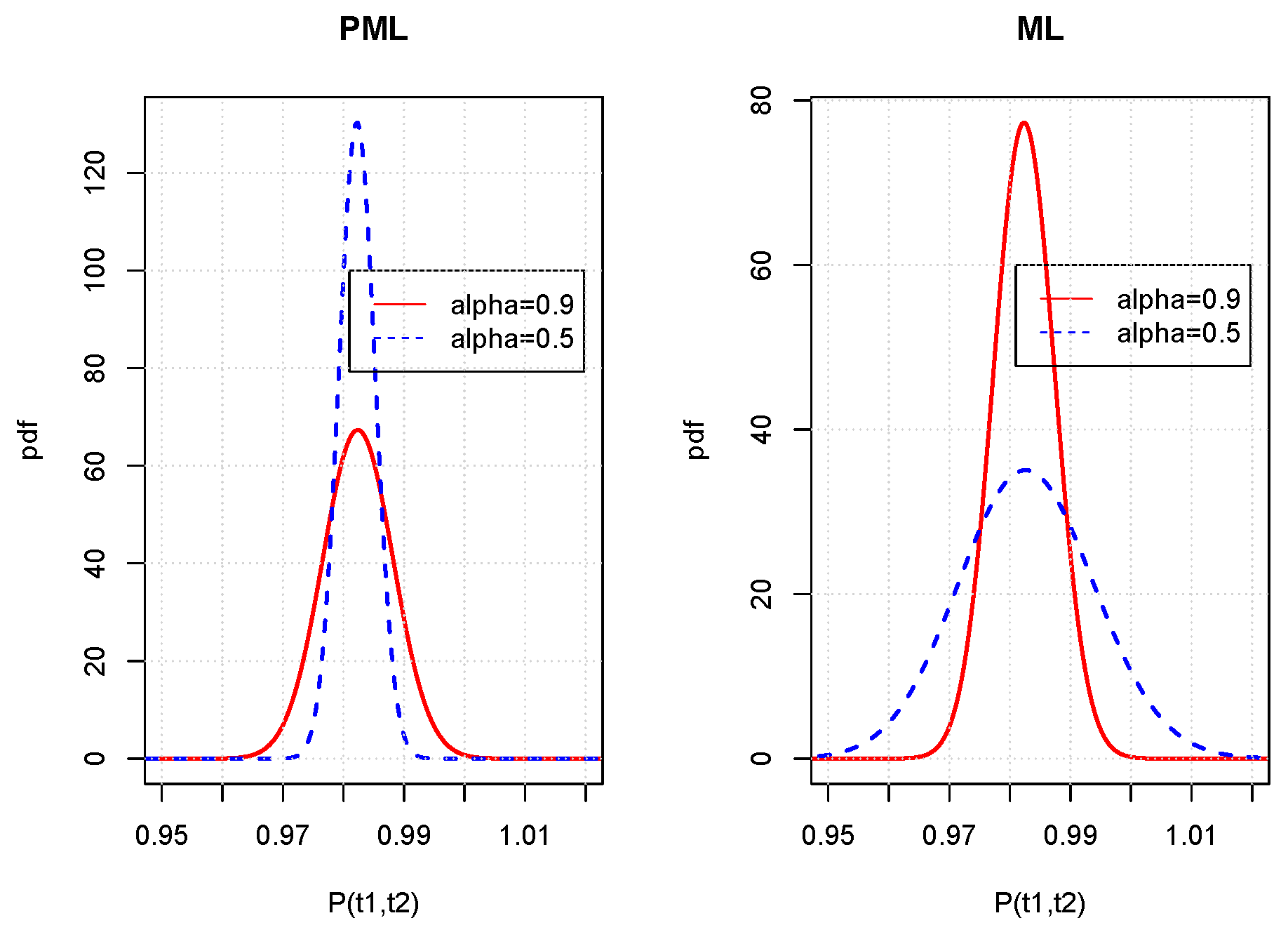
Figure 9 shows the probability density functions of $P^{\left(n\right)}(5,10)$ under the forward measure of numeraire $P^{\left(n\right)}(0,5)$. We consider for this illustration a one factor Lévy model ($d=1$) in which the driving process is a jump-diffusion such as presented in Equation (48), with the same parameters as those of Section 6. The DFT parameters are $x_{max}=0.2$ and $M=2^{10}$. The plots reveals that variances under $\mathbb{F}$ of bond prices display the same sensitivity to memory parameter $\alpha$ as under the risk of neutral measures. PML and ML bond variances are, respectively, directly and inversely proportional to $\alpha$.

After computation of the log-bond density, the call price is calculated by the following sum:

$$\begin{array}{ccc}\hfill C\left(s\right)& =& P(s,t_1){\mathbb{E}}^{\mathbb{F}}\left({\left(P(t_1,t_2)-K\right)}_{+}|{\mathcal{F}}_s\right)\hfill \\ & \approx & P(s,t_1)\sum _{k=1}^M{\mathbf{1}}_{\{x_k\ge lnK\}}\left(e^{x_k}-K\right)f^{\left(n\right)}\left(x_k\right){\Delta }_x,\hfill \end{array}$$

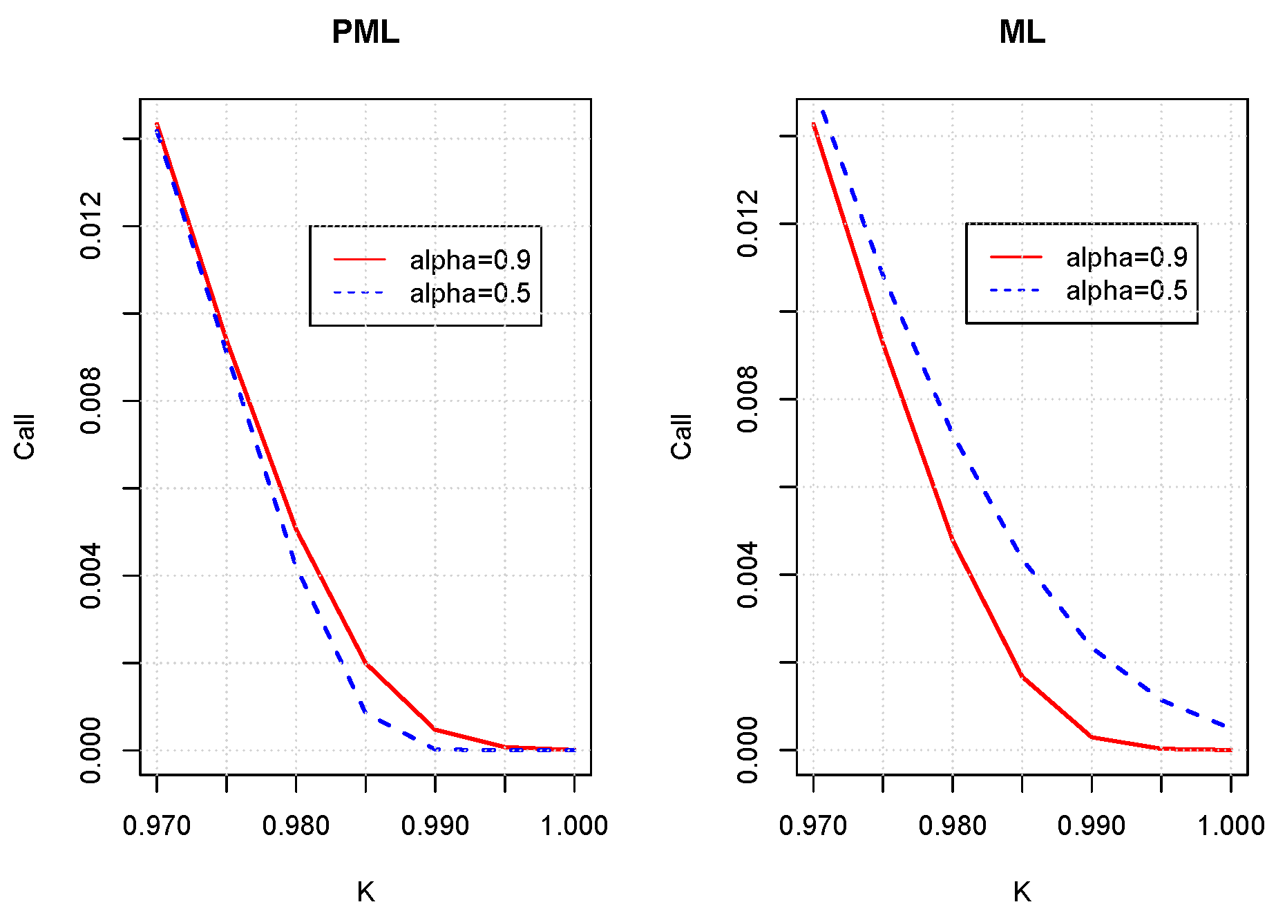
where ${\mathbf{1}}_{\{x_k\ge lnK\}}$ is an indicator variable equal to one on $[lnL,+\infty )$ and zero otherwise. Figure 10 shows call prices on $P^{\left(n\right)}(5,10)$ for various strike prices in ML and PML kernels. In the PML model, increasing the memory parameter $\alpha$ drives up the option values with respect to whatever the strike price is. For the ML kernel, we observed the opposite trend. This is relevant with our previous conclusions about the variance that is the main driving factor of option prices.

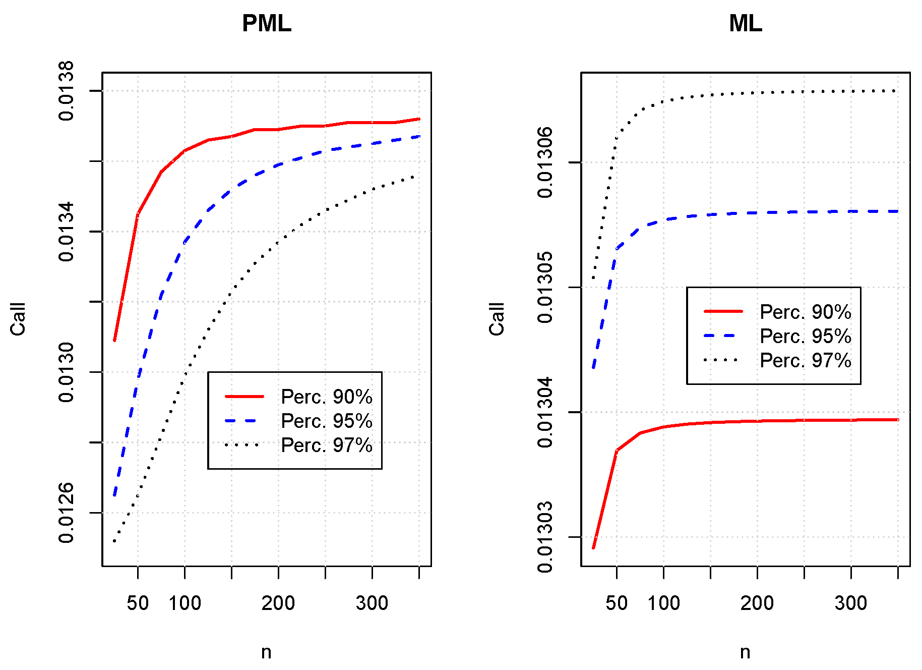
Figure 11 allows us to confirm the convergence of the call option when the number, n, of atoms in the discretization scheme grows. We recall that the partition ranges from ${\xi }_0=0$ up to ${\xi }_n$ that is a percentile of ${\gamma }_j\left(z\right)$. Here, percentiles 90%, 95% and 97% are considered. For the ML kernel (right plot), the convergence is quick and the difference between prices computed with the 90% and 97% is negligible (around 2.6 ${10}^{-5}$). For the PML model (left plot), prices are higher (and then conservative) with a 90% percentile and converge with less atoms than with a partition covering 97% of ${\gamma }_j(.)$.

8. Conclusions

This article contributes to the literature on interest rate models by proposing an alternative to standard mean reverting processes. The latter have an exponential decaying memory of the interest rate sample path. Motivated by observations of Section 3, our approach instead considers models in which the memory kernels are sub-exponential functions. In this setting, the short-term rate remembers its recent history for a longer period than in the exponential framework.

Even if the interest rate process is not Markovian anymore, the model preserves a high level of analytical tractability by taking advantage of the Laplace–Stieltjes representation of the memory function. The short-term rate can indeed be reformulated as an infinite dimensional Markov process. In this setting, bond prices admit closed form expressions and a discretization scheme allows inferring their dynamics. Furthermore, Section 7 proposes a procedure based on a change of numeraire to evaluate European bond options. The numerical analysis underlines the differences between models with Mittag–Leffler (ML) or power Mittag–Leffler (PML) memory kernels. The main one being that standard deviations of bond yields are, respectively, directly and inversely proportional to parameter $\alpha$.

This article paves the path for further research. For instance, the model could be adapted to a multi-curves framework or could serve as basis for a deeper empirical analysis. Other possible extensions are the modulation of parameters by a Markov chain to capture economic regimes or the introduction of clustered jumps.