Optimization of Electronic Nose Sensor Array for Tea Aroma Detecting Based on Correlation Coefficient and Cluster Analysis

Abstract

The electronic nose system is widely used in tea aroma detecting, and the sensor array plays a fundamental role for obtaining good results. Here, a sensor array optimization (SAO) method based on correlation coefficient and cluster analysis (CA) is proposed. First, correlation coefficient and distinguishing performance value (DPV) are calculated to eliminate redundant sensors. Then, the sensor independence is obtained through cluster analysis and the number of sensors is confirmed. Finally, the optimized sensor array is constructed. According to the results of the proposed method, sensor array for green tea (LG), fried green tea (LF) and baked green tea (LB) are constructed, and validation experiments are carried out. The classification accuracy using methods of linear discriminant analysis (LDA) based on the average value (LDA-ave) combined with nearest-neighbor classifier (NNC) can almost reach 94.44~100%. When the proposed method is used to discriminate between various grades of West Lake Longjing tea, LF can show comparable performance to that of the German PEN2 electronic nose. The electronic nose SAO method proposed in this paper can effectively eliminate redundant sensors and improve the quality of original tea aroma data. With fewer sensors, the optimized sensor array contributes to the miniaturization and cost reduction of the electronic nose system.

1. Introduction

Tea is one of the most popular non-alcoholic beverages in the world. Aroma is an important attribute of tea, which contains rich information such as quality and type. There are approximately 600 aromatic compounds in tea aroma [1,2]. At present, tea aroma detection depends primarily on the sensory evaluation of tea appraisers, which is time-consuming, labor-intensive and not conducive to ensuring accuracy. In recent years, electronic nose systems have played an increasingly important role in the field of gas detection. Electronic nose can closely mimic the organization of human olfactory system for obtaining the fingerprints of gas signals from samples through a sensor array, and pattern recognition methods have the ability to identify ‘fingerprints’ in a given dataset [3]. The sensor array composed of gas sensors is highly sensitive to the main volatile components in the target aroma sample. Therefore, the mapping from aroma to semantic information such as variety and grade can be constructed. Electronic nose has played an important role in many fields of food engineering, including food classification [4,5], quality assessment [6,7], freshness prediction [8] and identification authenticity [9]. Research objects include various foods such as fruit [10], vegetables [11], meat [12], beverage [13,14,15], herb [16] and especially tea [17,18,19,20,21,22].

The electronic nose system contains two main functional modules: sensor array and signal processing tool [17]. Many scholars have conducted research on the data analysis methods in the signal processing tool. Data processing is generally divided into two steps: feature extraction and recognition decision. At present, there are various modes for extracting features from original sensor signals, such as the maximum value [23], average value [24], integral value [25], differential value [26], maximum energy [27] and wavelet packet decomposition [28]. Different pattern recognition technologies are introduced to make recognition decisions, including multi-layer perceptron (MLP) [29], LDA [30], principal component analysis (PCA) [31], support vector machine (SVM) [32] and artificial neural network (ANN) [33]. These methods have achieved excellent results in specific application scenarios. It is worth noting that although a complex method can extract as much information as possible and improve the accuracy, it will increase the discrimination time. The simple method may sacrifice accuracy. If you want to achieve a win-win of efficiency and performance, higher requirements are placed on the quality of the original signal.

Since the sensor array plays a fundamental role in acquiring good original data for detection, some studies focus on sensor array optimization (SAO). In short, the purpose of SAO is to use the fewest sensors to extract the most distinguishable signals for subsequent data processing [34]. This goal can be achieved by using dedicated sensors for given volatile substances. Chen et al. [35] conducted cluster analysis of variance difference matrix to identify several possible sensor subsets for Chinese medicine. Zhou et al. [36] applied PCA and load factor analysis to select sensors with small inter-class dispersion and large intra-class dispersion, respectively, of the sensor’s data or their eigenvalues. However, they consider the inter- and the intra-class dispersion indices separately, which cannot reflect the sensors’ comprehensive identification performances. Bhattacharyya et al. [4] and Xu et al. [7] perform sensor screening based on the response value of a specific chemical signal. But this method can only guarantee sensitivity, not distinguishability. From the above research, we can conclude that most of the SAO studies consider the selection and construction of sensor arrays based on sensor sensitivity or correlation between sensors. However, only considering the correlation index between sensors is not enough. Secondly, the number of sensors included in the array will also have an important impact on the performance and cost of the sensor array, but there are few studies in this area.

In this paper, a two-step down-selection SAO method is proposed. Three kinds of sensor arrays for green tea, fired green tea and baked green tea are constructed. Combining five pattern recognition methods, the effectiveness of the constructed sensor array in identifying the types and grades of green tea was verified. Sensor arrays based on other SAO strategies and the number of sensors were also constructed to prove the superiority of the proposed method from different perspectives. The proposed method provides a more effective idea and potential solution for the construction of gas sensor array.

2. Materials and Methods

2.1. Tea Samples Preparation

In China, there are 4 kinds of green tea: fried green tea, baked green tea, sunburned green tea and steamed green tea. Among them, fried and baked green tea occupy the main market share. Hence, we mainly focus on fried green tea and baked green tea.

The tea samples for SAO consist of 3 kinds of fried green tea, i.e., maoshanqingfeng (msqf), dinggudafang (dgdf) and queshe (qs), and 3 kinds of baked green tea, i.e., luanguapian (lagp), huangshanmaofeng (hsmf) and taipinhoukui (tphk).

Three other kinds of fried green tea, shangwushanhuibai (swshb), laoshanlvcha (lslc) and biluochun (blc), and three other kinds of baked green tea, jingtinglvxue (jtlx), hanzhongxianhao (hzxh) and emeishanmaofeng (emsmf), are used to validate the discriminating performance of the optimized sensor array for green tea. The tea samples are given in

Table 1. Detailed information of green tea samples.

Processing Technology	Fried Green Tea			Baked Green Tea
Tea samples for training	msqf	dgdf	qs	lagp	hsmf	tphk
Place	Changzhou	Huangshan	Hefei	Huangshan	Huangshan	Huangshan
Date	03/2018	03/2018	04/2018	03/2018	03/2018	04/2018
Tea samples for validation	swshb	lslc	blc	jtlx	hzxh	emsmf
Place	Shengzhou	Qingdao	Suzhou	Xuancheng	Xi’an	Chengdu
Date	04/2020	04/2020	04/2020	04/2020	04/2020	04/2020

.

As one of the representative brands of fried green tea in China, the grades classification of West Lake Longjing has also received great attention. Hence, 4 grades of West Lake Longjing are also used to validate the discriminating performance of the optimized sensor array for fried green tea.

The experimental parameters of the sample preparation and aroma collection can affect the reaction speed, which subsequently affects the final detection effect. Hence, some preliminary experiments were carried out to select the optimal experimental parameters including sealing time, gas flow rate, temperature and data acquisition time. The tea aroma sampling process is as follows:

The ambient temperature is maintained at 25 °C. In the 500 mL beaker, 5 g of tea leaves is brewed with 250 mL of boiling water. The water is then poured out after 5 min and leaves the tea at the bottom of the cup. The beaker is sealed for 30 min until the tea aroma is volatile. Then, the air pump pumps the aroma evenly into the electronic nose system at a flow rate of 15 mL/s, and flows through the sensor array. The stable response value after 35 s is used for analysis, and the response values of each sensor are read every second for approximately 60 s. There are 3 samples of each kind of tea, and each sample is measured once. Since a drying tube was added before the aroma entered the reaction chamber, indoor humidity had little effect on the experimental results. Hence, there are no special considerations regarding humidity in this paper.

The response curve of a typical green tea (West Lake Longjing) is shown in Figure 1. Each curve represents the variation in conductivity of each sensor with time when the tea volatiles reached the reaction chamber. It can be seen that in the 35–60 s interval, the response values of all sensors tend to be stable. In subsequent experiments, we observed that all tea aroma samples used in this study have similar characteristics, so it is reasonable to use the response value in the same interval for subsequent feature extraction and pattern recognition.

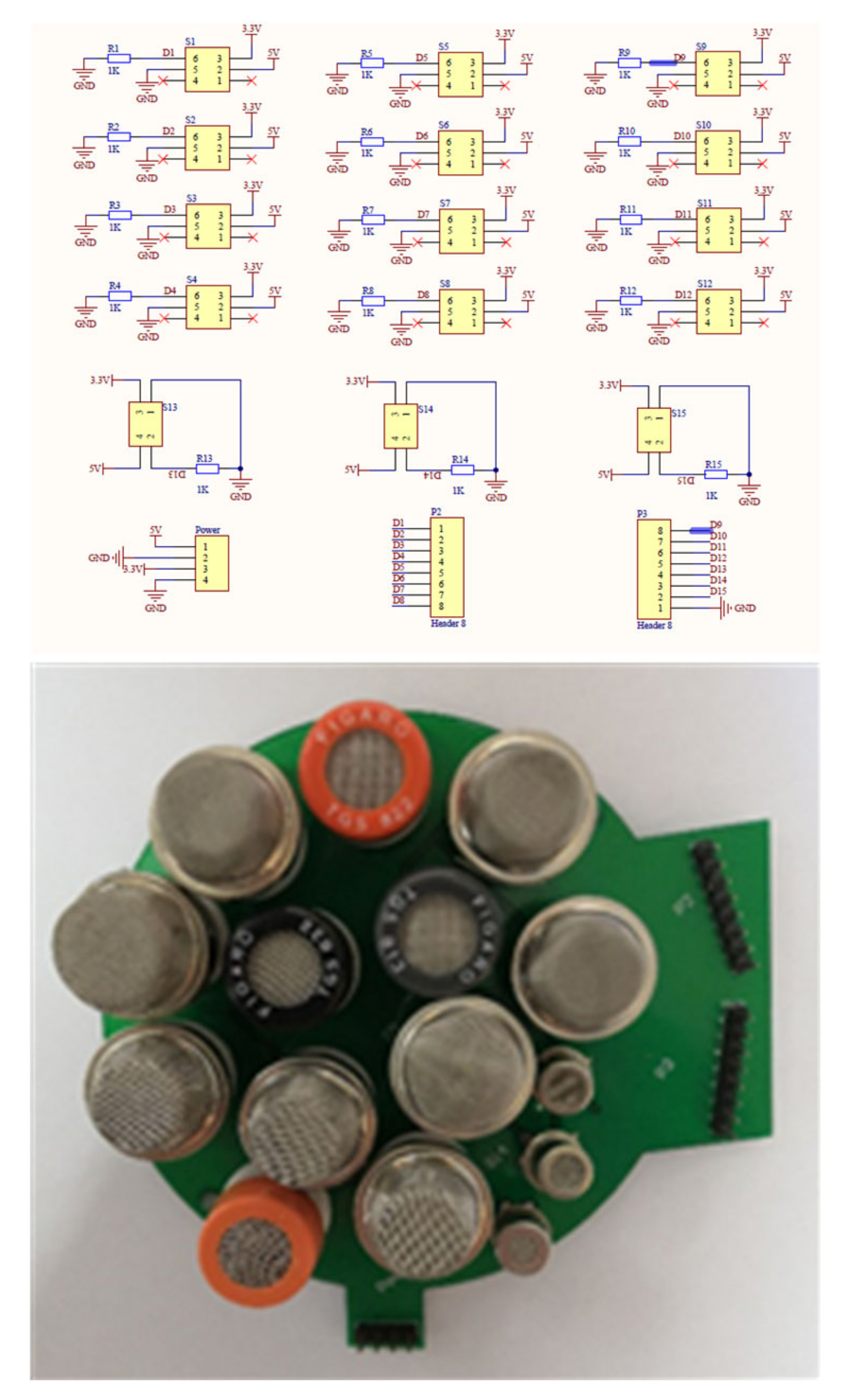
2.2. Preliminary Sensor Array

First, we conduct a preliminary screening of common gas sensors on the market to construct a candidate list. The sensors are selected according to the following three criteria: (1) sensors sensitive to aroma components; (2) sensors used in other studies regarding odor detection; and (3) sensors with stable performances and full ranges of models. Based on the above 3 criteria, the gas sensors were finally selected. Those sensors have the operating voltage (5 V) and external resistance necessary to facilitate the integrated circuit design of the sensor. The preliminary sensors and their basic information are shown in

Table 2. Detailed information of preliminary sensors.

Scheme	Sensitivity to Gases	Heating Resistance/Ω
TGS813	Isobutane, propane, ethanol, methane, etc.	30.0 ± 3.0
TGS822	Acetone, ethanol, benzene, ethane, etc.	38.0 ± 3.0
TGS2600	Hydrogen sulfide gas	≈83.0
TGS2620	Organic solvents	≈83.0
MQ-6	Olefins, 2 to 4 carbon alkanes	26.0 ± 3.0
MQ-5	Combustible gas	31.0 ± 3.0
TGS832	Halogenated hydrocarbons, alcohols	30.0 ± 3.0
TGS826	Ammonia	30.0 ± 3.0
TGS2610	Hydrogen sulfide gas	≈59.0
2M009	Toluene and benzene gas	33.0 ± 3.0
MQ-8	Diethyl ether	31.0 ± 3.0
MQK2	Methanol, ethanol gas	31.0 ± 3.0
2M012	Hydrogen	33.0 ± 3.0
MQ-3	Ethanol vapor	29.0 ± 3.0
TGS800	Methane, isobutane, hydrogen, etc.	38.0 ± 3.0

; more details are in Table S1 in the Supplementary Files.

All sensors listed in Table 2 are metal oxide sensors (MOSs). As an example, the circuit schematic of sensor TGS826 is shown in Figure 2. It requires two voltage sources: heating voltage (V_H) and loop voltage (V_C). V_H can keep the sensor at a certain temperature, and V_C can monitor the voltage (V_RL) across the load resistance (R_L). When the sensors detect sensitive gases, the resistance of the sensor decreases, and the voltage across the load resistance increases.

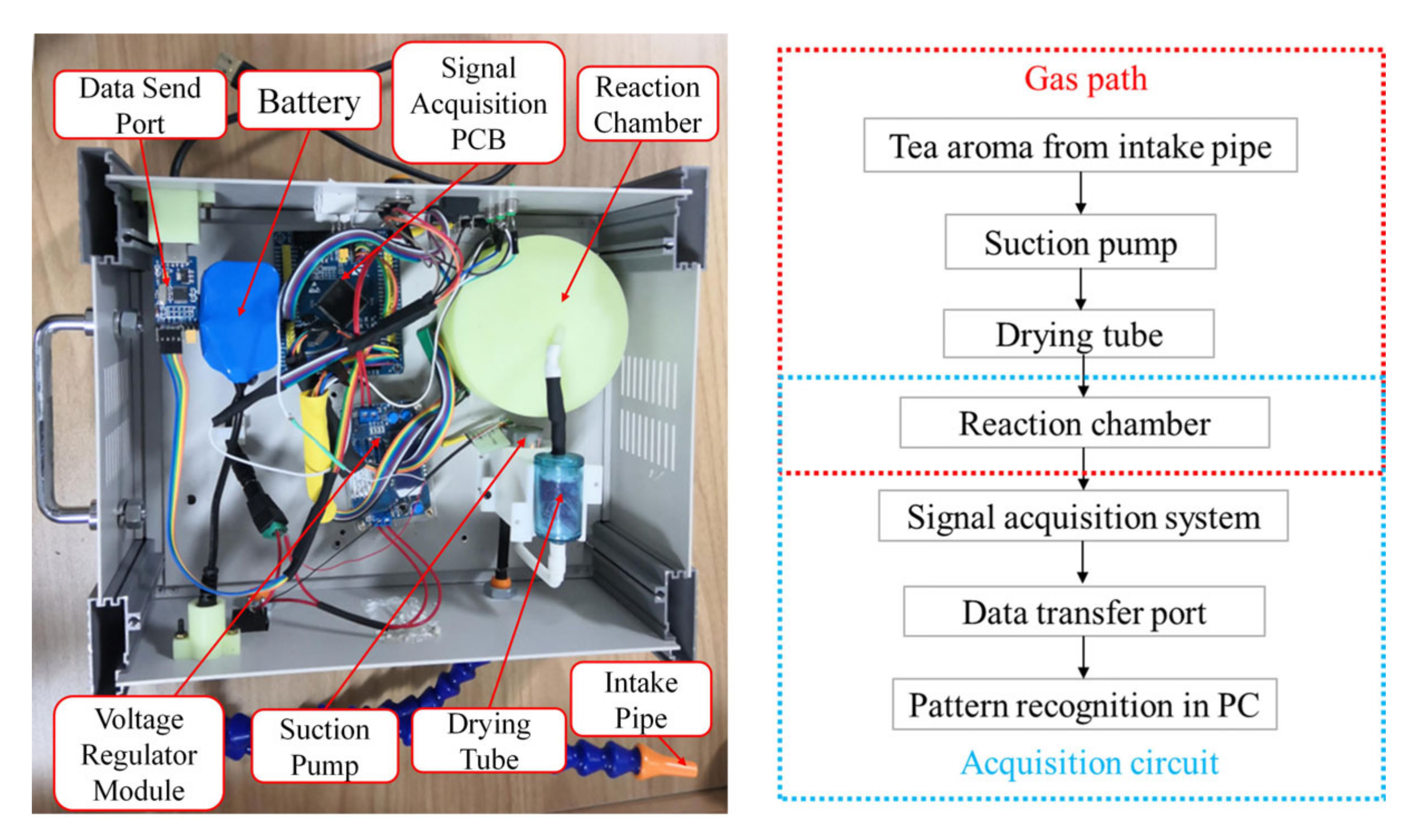
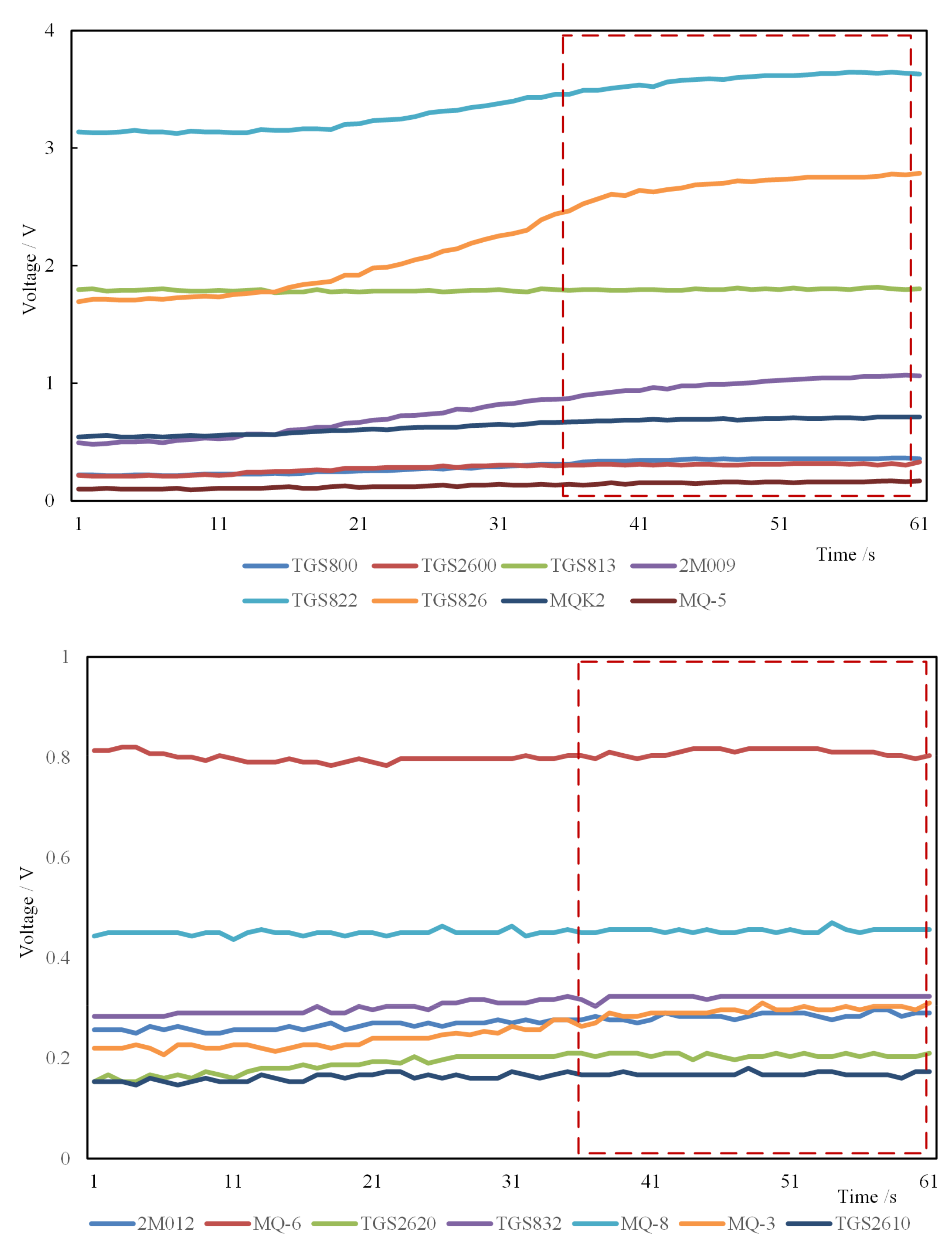
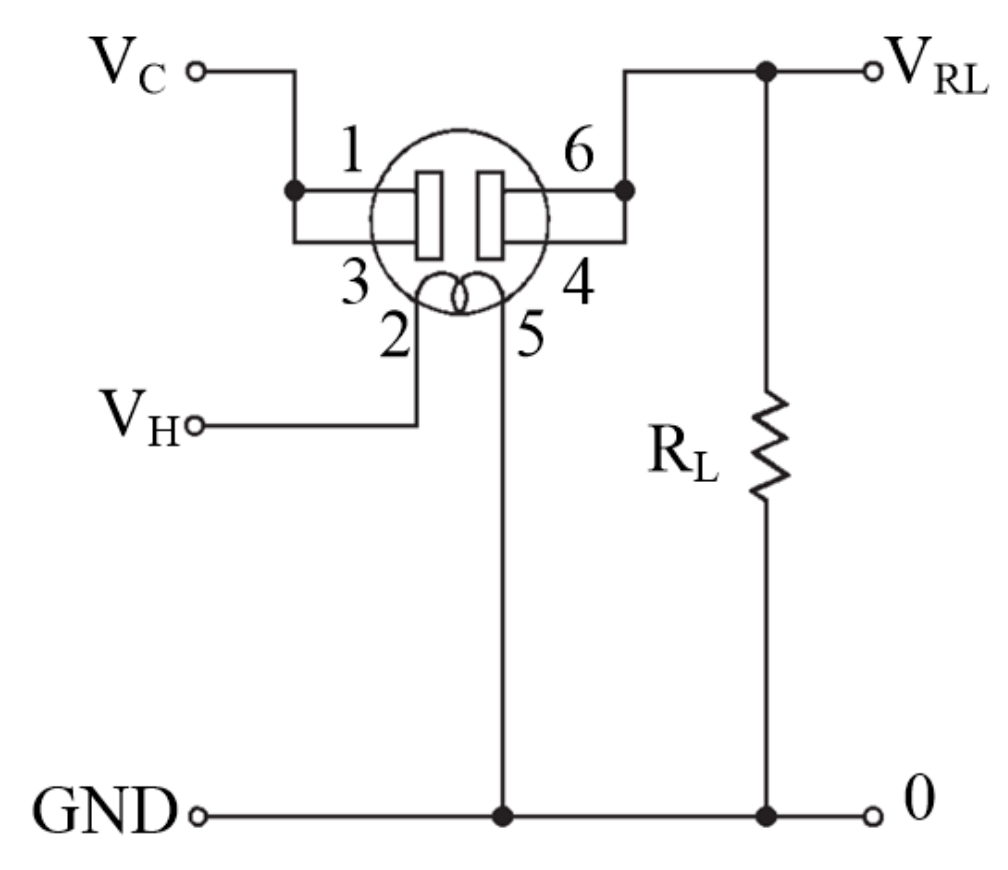
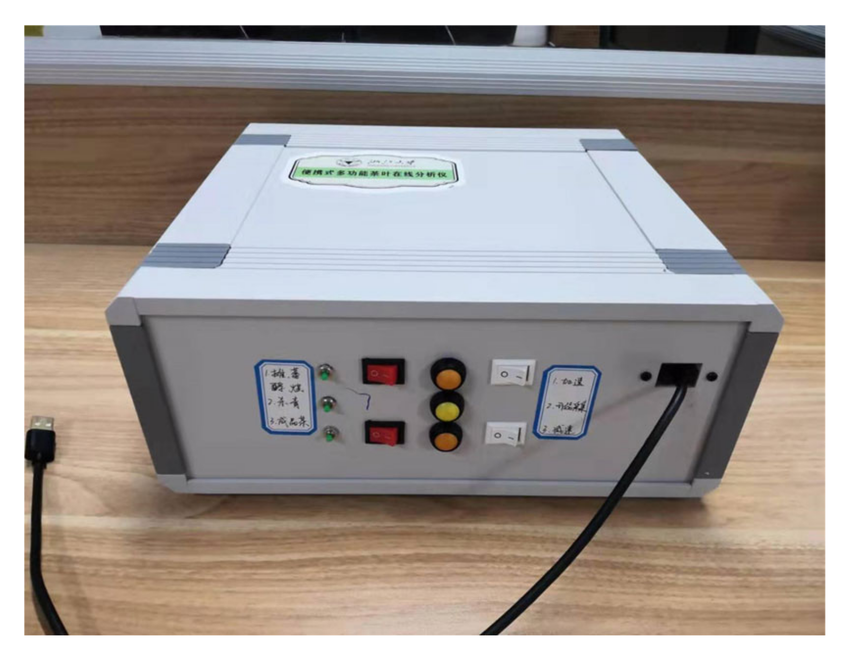
2.3. Electronic Nose System Set-Up

The self-made electronic nose system used was primarily composed of a gas path and a signal acquisition circuit. The internal structure and airflow of the device are shown in Figure 3. An introduction of all of the components of the e-nose system can be seen in Table S2 in the Supplementary Files. The workflow of the device is as follows:

(1) After the samples are ready, the aroma is pulled out by the suction pump and then flowed into the drying tube. The drying tube is filled with sufficient amount of granular silica gel desiccant (produced by Longhui Desiccant Co., Ltd., Suzhou, Jiangsu Province, China). Hence, the water vapor in the tea aroma is removed to prevent it from affecting the measurement result.

(2) The aroma enters the reaction chamber and reacts with the sensors to generate a response signal. The reaction chamber is made of acrylonitrile butadiene styrene (ABS) and is 3D printed, which has high strength and good heat insulation. The reaction chamber is especially designed to ensure that the aroma environment of each sensor in the sensor array is uniform and consistent.

(3) The signal acquisition circuit can obtain the response signal and send it to the host analysis system in a personal computer (PC) through the serial port. The post-processing and pattern recognition of the signal are completed in the PC.

The schematic and an image of the sensor array are shown in Figure 4. In the schematic, s1–s15 indicates the 15 sensors; p2 and p3 indicate the sensors’ signal extraction pins. The overall appearance of the electronic nose system is shown in Figure 5. The overall size of the e-nose system is 300 mm × 200 mm × 110 mm. All function modules are integrated in the gray box. There are some function buttons on the operation panel, which provide functions such as power switch, flow adjustment, pre-heating and purging.

2.4. Data Analysis Methods

Two kinds of features, average value and value on the maximum variance moment, are extracted from the original sensor response curve. The calculation of the average value is shown in Equation (1):

$$m_n^{\prime }=\frac{{\displaystyle \sum _{T=1}^k{m}_{nT}}}{k}$$

(1)

where k is the number of sampling, n is the number of sensors and $m_{nT}$ is the response value of the nth sensor at time T. $m_n^{\prime }$ is the average value of the nth sensor for the sample, which will eventually form a feature vector of 1 × n dimension.

For the second method, the variance of all sensors at the same time is calculated firstly; the calculation method is shown in Equation (2). Then, the response value of each sensor at the time when the variance value is maximum is found out, forming a 1 × n dimensional feature vector.

$$S^2=\frac{{\displaystyle \sum _{i=1}^n{(m_{iT}-{\overline{m}}_{iT})}^2}}{n-1}$$

(2)

where n is the number of sensors, $S^2$ is the variance and $m_{iT}$ represents the response value of the i-th sensor at time T.

Two simple and widely-used pattern recognition methods, principal component analysis (PCA) and linear discriminant analysis (LDA), are introduced for data processing after feature extraction. PCA could deduct dimensions and observe a primary evaluation of the between-class similarity. PCA is a projection method that allows an easy visualization of all the information contained in a dataset. LDA is a statistical method that could determine to which group the samples belong. The method maximizes the variance between categories and minimizes the variance within categories. With the help of dimensionality reduction and visualization of PCA and LDA, we can directly observe the distribution of samples of different categories.

In order to quantitatively compare the accuracy of different pattern recognition methods in discriminating unknown samples, the nearest neighbor classifier (NNC) is introduced for category discrimination. For each category participating in the discrimination, 3 additional aroma samples were collected as a test set. The original 3 samples are used as labeled data for training to build the model.

In a previous work, the authors introduced the random forest machine learning (RFML) algorithm to analyze aroma data and achieved excellent performance [15], and it is also introduced for comparative research. Taking the random sampling of RFML into account, we repeated the same unknown sample discrimination experiment 10 times, and took the average value as the final accuracy result.

2.5. Sensor Array Optimization Methods

The two-step down-selection methodology of SAO involves the analysis of the following factors (the flow chart of the method is shown in Figure 6):

(1) Correlation analysis. The correlation coefficient between the two sensors is calculated. The large value of the correlation coefficient means that the two sensors have a strong correlation, and the obtained signals have high similarity. Thus, the two sensors can replace each other. The correlation coefficient can be calculated using Equation (3):

$$\left|R_{xy}\right|=\left|\frac{{\displaystyle {\sum }_{i=1}^N\left(x_i-\overline{x}\right)\left(y_i-\overline{y}\right)}}{\sqrt{{{\displaystyle {\sum }_{i=1}^N{\left(x_i-\overline{x}\right)}^2\left(y_i-\overline{y}\right)}}^2}}\right|$$

(3)

where x and y represent two different models of sensors; $\overline{x}$ and $\overline{y}$ are the mean value of the first 60 s of the two sensors, respectively; $x_i$ is the i-th data value of the x sensor, $y_i$ is the i-th data value of the y sensor, and $\left|R_{xy}\right|$ is the absolute value of the correlation coefficient between sensor x and sensor y.

(2) Distinguishing performance value (DPV) calculation. Only one of the replaceable sensors can be kept. It is difficult to make this decision based solely on the sensitivity of the sensor. Therefore, the ability of the sensor to discriminate among different tea classes can be determined by calculating the inter- and intra-class dispersion, that is, the DPV. Sensors with smaller DPVs should be eliminated. The DPV of each sensor was evaluated by calculating the inter- and the intra-class dispersion, as shown in Equation (4):

$$F_{\mathrm{i}}=\frac{S_b}{S_w}=\frac{\frac{1}{n}{\displaystyle {\sum }_{i=1}^n\left(u_i-u\right)}{\left(u_i-u\right)}^T}{\frac{1}{n}\times \frac{1}{m}{\displaystyle {\sum }_{i=1}^n{\displaystyle {\sum }_{k=1}^m\left(u_i-x_k\right){\left(u_i-x_k\right)}^T}}}$$

(4)

where S_b and S_w are the inter- and intra-class dispersions of the sample, respectively. A larger F_i value represents better distinguishing performance. n denotes the number of tea varieties, m is the number of samples for detecting of each tea variety, u denotes the average detected value of total tea samples, u_i denotes the average detected value of total samples of tea variety i, and x_k denotes the detected value of the k-th sample of tea variety i.

(3) Cluster analysis (CA). In the process of constructing the sensor array, the independence between the sensors should be considered. Through CA, the distance between different sensors can be calculated to determine the independence between the sensors.

(4) Sensor number determination. If the number of sensors N in the array is not specified, the effect of tea aroma detection is tested with a different number N of sensor arrays, and N is determined based on the effect.

3. Results and Discussions

3.1. Sensor Array Optimization Results

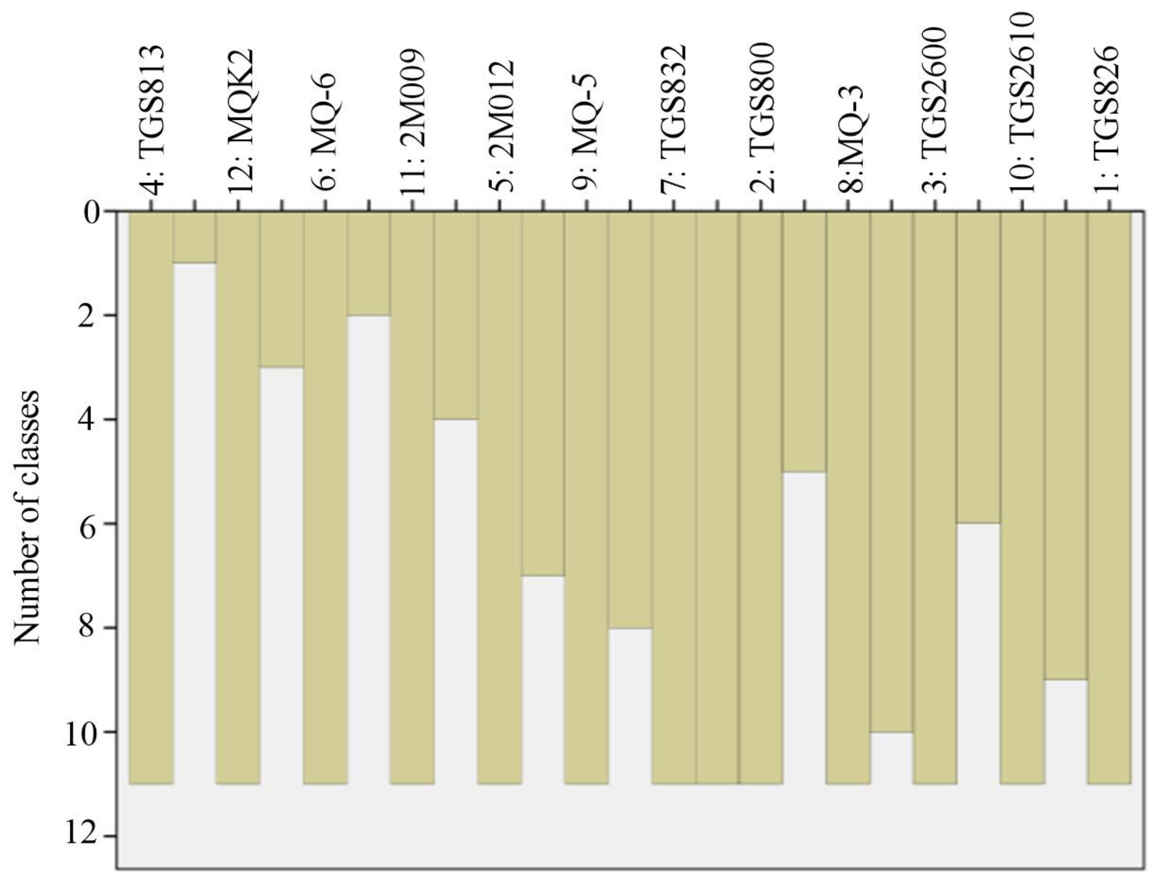
3.1.1. Optimization of Sensor Array LG for Green Tea

(1) Sensor array optimization based on correlation analysis and the DPV

Correlation analysis is used to calculate the correlation coefficient between two sensors. The correlation coefficient $R_{xy}$ ranges from −1 to 1, and $R_{xy}\ge 0$ means positive correlation and vice versa. The degree of correlation of the sensor increases as $\left|R_{xy}\right|$ increases. When $\left|R_{xy}\right|$ ≥ 0.9, we can believe that the two sensors have strong similarity and can replace each other. If there is no $\left|R_{xy}\right|$ ≥ 0.9 in detecting a certain tea variety, we also take three sensor pairs with the largest $\left|R_{xy}\right|$ as the candidates to be removed.

Table 3. Sensors with high correlation coefficient in detecting a certain tea.

msqf		dgdf		qs
Sensor model	$\left|R_{xy}\right|$	Sensor model	$\left|R_{xy}\right|$	Sensor model	$\left|R_{xy}\right|$
TGS826/TGS822	0.96	TGS832/TGS2620	0.98	MQK2/TGS822	0.95
MQK2/TGS822	0.97	TGS822/TGS813	0.96	TGS822/MQ-8	0.92
TGS2620/TGS822	0.95	MQ-8/TGS822	0.93	MQ-6/MQK2	0.91
TGS822/2M009	0.96	TGS813/MQ-8	0.90	MQ-6/TGS822	0.91
TGS2620/MQK2	0.95	TGS826/TGS813	0.93	MQ-8/MQK2	0.93
lagp		hsmf		tphk
Sensor model	$\left|R_{xy}\right|$	Sensor model	$\left|R_{xy}\right|$	Sensor model	$\left|R_{xy}\right|$
MQ-6/2M012	0.88	MQ-6/TGS822	0.96	MQ-3/TGS832	0.92
MQ-3/2M012	0.88	MQ-6/MQ-5	0.90	MQ-6/TGS832	0.86
MQ-3/MQ-6	0.88	TGS822/MQ-5	0.87	MQ-6/MQ-3	0.86

shows a list of sensor pairs with $\left|R_{xy}\right|\ge 0.9$ or maximum three values of $\left|R_{xy}\right|$ in different tea aromas.

Since the selected sensors are sensitive to tea aroma, it is not easy to decide which to eliminate based on the sensitivity of the sensors. Thus, the DPV of each sensor was evaluated by calculating the inter- and the intra-class dispersion.

Table 4. Sensors’ DPVs for different kinds of green tea.

Sensors	DPVs for 6 General Green Teas	Ranking	DPVs for 3 Fried Green Teas	Ranking	DPVs for 3 Baked Green Teas	Ranking
TGS826	4.59	9	0.32	9	0.25	9
TGS800	0.17	15	0.15	14	0.16	12
TGS2600	3.89	11	0.27	10	0.12	13
TGS813	65.21	6	0.5965	6	0.67	6
2M012	218.39	4	22.37	2	0.186	11
MQ-6	189.95	5	40.51	1	1.21	5
TGS832	6.56	8	0.26	11	5.87	2
TGS2620	1.64	13	0.14	15	0.65	7
TGS822	13.74	7	0.1896	12	1.94	4
MQ-8	1279.00	1	0.58	8	12.73	1
MQ-3	401.99	3	2.16	3	0.30	8
MQ-5	2.06	12	0.82	5	0.05	14
TGS2610	1.28	14	0.5964	7	0.195	10
2M009	4.32	10	0.1891	13	0.01	15
MQK2	1278.08	2	1.16	4	3.56	3

shows the sensors’ DPVs for 6 kinds of green tea, including 3 kinds of fried green tea and 3 kinds of baked green teas. Significant differences in the DPVs occur when different sensors detect tea aroma within identical varieties. When $\left|R_{xy}\right|$ of two sensors is high, as listed in Table 3, a redundant sensor can be eliminated. For example, the high correlated sensors TGS826/TGS822 for msqf and their DPVs for 6 general green teas are 4.59 and 13.74, respectively. Therefore, TGS826 needs to be eliminated due to its small DPV. Similarly, for detecting msqf, TGS822, TGS2620, 2M009 and TGS2620 should be respectively eliminated in the corresponding high correlated sensor pairs of MQK2/TGS822, TGS2620/TGS822, TGS822/2M009 and TGS2620/MQK2.

Due to the contingency of the detection, only sensors that are rejected by two or more kinds of green tea should be eliminated from sensor array LG for general green tea. Therefore, TGS826 and TGS2620 are eliminated since they are rejected in the detection of msqf and dgdf; TGS822 is eliminated since it is rejected in the detection of msqf, dgdf, qs and hsmf; MQ-6 is eliminated since it is rejected in the detection of qs, lagp and tphk. Hence, 11 sensors of 2M009, TGS813, TGS832, MQ-8, MQ-5, MQ-3, 2M012, TGS2600, TGS2610, MQK2 and TGS800 are retained. The optimization results are shown in

Table 5. Optimized sensor array LG for general green teas.

Tea Varieties	Sensors Retained in the Array	Sensors Eliminated
msqf	TGS813, TGS832, MQ-6, MQ-8, MQ-5, MQ-3, 2M012, TGS2600, TGS2610, MQK2, TGS800	TGS826, TGS822, TGS2620, 2M009
dgdf	2M009, TGS832, MQ-6, MQ-8, MQ-5, MQ-3, 2M012, TGS2600, TGS2610, MQK2, TGS800	TGS826, TGS2620, TGS813, TGS822
qs	2M009, TGS813, TGS832, MQ-8, MQ-5, MQ-3, 2M012, TGS2620, TGS2600, TGS2610, TGS826, TGS800	TGS822, MQ-6, MQK2
lagp	2M009, TGS813, TGS822, TGS832, MQ-8, MQ-5, MQ-3, TGS2620, TGS2600, TGS2610, TGS826, MQK2, TGS800	MQ-6, 2M012
hsmf	2M009, TGS813, TGS832, MQ-6, MQ-8, MQ-3, 2M012, TGS2620, TGS2600, TGS2610, TGS826, MQK2, TGS800	TGS822, MQ-5
tphk	2M009, TGS813, TGS822, MQ-8, MQ-5, MQ-3, 2M012, TGS2620, TGS2600, TGS2610, TGS826, MQK2, TGS800	MQ-6, TGS832

.

(2) Sensor array optimization based on CA and DPV

The previous step eliminated redundant sensors with high correlation through correlation analysis and the DPV. However, how to select a specific number of (N) sensors from the remaining sensors to construct the array is still unknown. Thus, CA and the DPV are designed to solve this problem.

The average value of aroma response data of each sensor to each sample of different tea varieties was used as input. The system cluster method was performed. The square Euclidean distance was used as the measurement standard and the between-groups linkage was used as cluster method to analyze the output icicles of cluster results. The whole process was performed in SPSS 24.0 software. The results are shown in Figure 7. The clustering coefficients between the sensors are shown in

Table 6. Clustering coefficient among sensors.

Ranking	Sensor Group		Value
1	TGS800	MQ-5	0.002
2	TGS2600	TGS2610	0.006
3	TGS800	TGS832	0.047
4	TGS800	TGS2600	0.080
5	MQ-3	2M009	0.381
6	TGS800	2M012	0.490
7	TGS800	MQ-3	2.296
8	TGS813	MQ-8	2.911
9	TGS800	TGS813	22.894
10	TGS800	MQK2	28.746

.

According to Figure 7, if the histograms of the sensors are connected, the connected sensors can be grouped into one class. For example, if we want to group the sensors into 8 classes, we can make a horizontal dotted line at the place with the ordinate of 8 (shown in Figure 7). By scanning left to right, the continuous sensor histogram without disconnection can be grouped into one class, and the results of 8 classes can be obtained, namely MQK2, MQ-8, TGS813, 2M009, MQ-3, 2M012, (TGS2610/TGS2600) and (TGS832/MQ-5/TGS800). Similarly, we can cluster the remaining 11 sensors into 2–10 classes, as shown in

Table 7. CA results and optimized sensor array with different number N by CA and DPV.

Clusters Number	CA Results	Optimized Sensor Arrays with Different Number N by CA and DPVs
2	MQK2, (MQ-8/TGS813/2M009/MQ-3/ 2M012/TGS2610/TGS2600/TGS832/MQ-5/TGS800)	MQK2, MQ-8
3	MQK2, (MQ-8/TGS813), (2M009/MQ-3/ 2M012/TGS2610/TGS2600/TGS832/MQ-5/TGS800)	MQK2, MQ-8, MQ-3
4	MQK2, MQ-8, TGS813, (2M009/MQ-3/ 2M012/TGS2610/TGS2600/TGS832/MQ-5/TGS800)	MQK2, MQ-8, TGS813, MQ-3
5	MQK2, MQ-8, TGS813, (2M009/MQ-3), (2M012/TGS2610/TGS2600/TGS832/MQ-5/TGS800)	MQK2, MQ-8, TGS813, MQ-3, 2M012
6	MQK2, MQ-8, TGS813, (2M009/MQ-3),2M012, (TGS2610/TGS2600/TGS832/MQ-5/TGS800)	MQK2, MQ-8, TGS813, MQ-3, 2M012, TGS832
7	MQK2, MQ-8, TGS813, 2M009,MQ-3, 2M012, (TGS2610/TGS2600/TGS832/MQ-5/TGS800)	MQK2, MQ-8,TGS813, 2M009, MQ-3, 2M012, TGS832
8	MQK2, MQ-8, TGS813, 2M009, MQ-3, 2M012, (TGS2610/TGS2600), (TGS832/MQ-5/TGS800)	MQK2, MQ-8, TGS813, 2M009, MQ-3, 2M012, TGS2600, TGS832
9	MQK2, MQ-8, TGS813, 2M009,MQ-3, 2M012, (TGS2610/TGS2600), TGS832, (MQ-5/TGS800)	MQK2, MQ-8, TGS813, 2M009, MQ-3, 2M012, TGS2600, TGS832, MQ-5
10	MQK2, MQ-8, TGS813, 2M009,MQ-3, 2M012, TGS2610, TGS2600, TGS832, (MQ-5/TGS800)	MQK2, MQ-8, TGS813, 2M009, MQ-3, 2M012, TGS2610, TGS2600, TGS832, MQ-5

.

For each clustered sensor class, we selected a sensor with maximum DPV in its class to construct the optimized sensor array. For example, if we want to obtain an optimized sensor array with number N = 8, there are two classes that have more than one sensor in the clustered results of 8 classes, namely (TGS2610/TGS2600) and (TGS832/MQ-5/TGS800). According to Table 5, the DPVs for 6 green teas of these sensors are ((TGS2610, 1.28)/(TGS2600, 3.89)) and ((TGS832, 6.56)/(MQ-5, 2.06)/(TGS800, 0.17)). Hence, we chose TGS2600 and TGS832 combined with other clustered classes with single sensor MQK2, MQ-8, TGS813, 2M009, MQ-3, 2M012 to construct an optimized sensor array with number N = 8. We can obtain optimized sensor arrays with different number N = 2–10 by CA and DPVs, as shown in Table 7.

(3) Sensor number determination

Table 8. Sensor arrays with different numbers N based on CA and DPV.

Number of Sensors (N)	Sensor Arrays Optimized by CA and DPV	Discrimination Accuracy by RFML [18]
2	MQK2, MQ-8	93.84%
3	MQK2, MQ-8, MQ-3	94.35%
4	MQK2, MQ-8, TGS813, MQ-3	96.09%
5	MQK2, MQ-8, TGS813, MQ-3, 2M012	97.07%
6	MQK2, MQ-8, TGS813, MQ-3, 2M012, TGS832	98.42%
7	MQK2, MQ-8, TGS813, 2M009, MQ-3, 2M012, TGS832	98.88%
8	MQK2, MQ-8, TGS813, 2M009, MQ-3, 2M012, TGS2600, TGS832	98.90%
9	MQK2, MQ-8, TGS813, 2M009, MQ-3, 2M012, TGS2600, TGS832, MQ-5	98.80%
10	MQK2, MQ-8, TGS813, 2M009, MQ-3, 2M012, TGS2610, TGS2600, TGS832, MQ-5	98.87%

shows the discriminating accuracy of six kinds of green tea (msqf, dgdf, qs, lagp, hsmf and tphk) by sensor arrays with different number N of sensors. In general, if N is too small, such as when N < 6, the accuracy will be relatively low. When N ≥ 6, the accuracy is more than 98%, and is very close to other rates, which are 98.42%, 98.88%, 98.90%, 98.80% and 98.87% for the accuracy rates of N = 6, 7, 8, 9 and 10, respectively. It can be seen that when N = 8, the number of sensors is appropriate and the accuracy is stable and relatively high. Thus, we can acquire an optimized array LG with 8 sensors MQK2, MQ-8, TGS813, 2M009, MQ-3, 2M012, TGS2600 and TGS832) for general green tea detection.

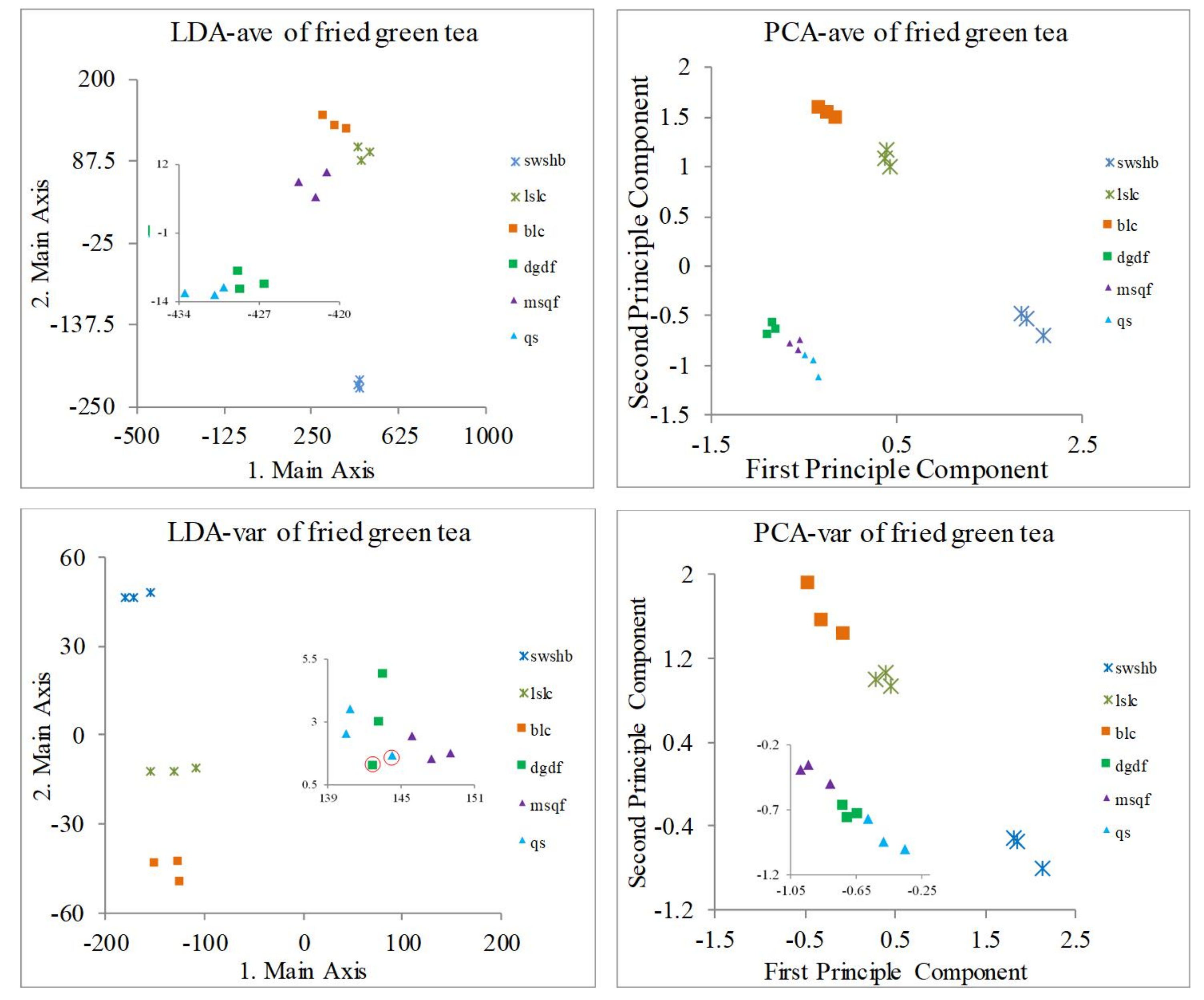
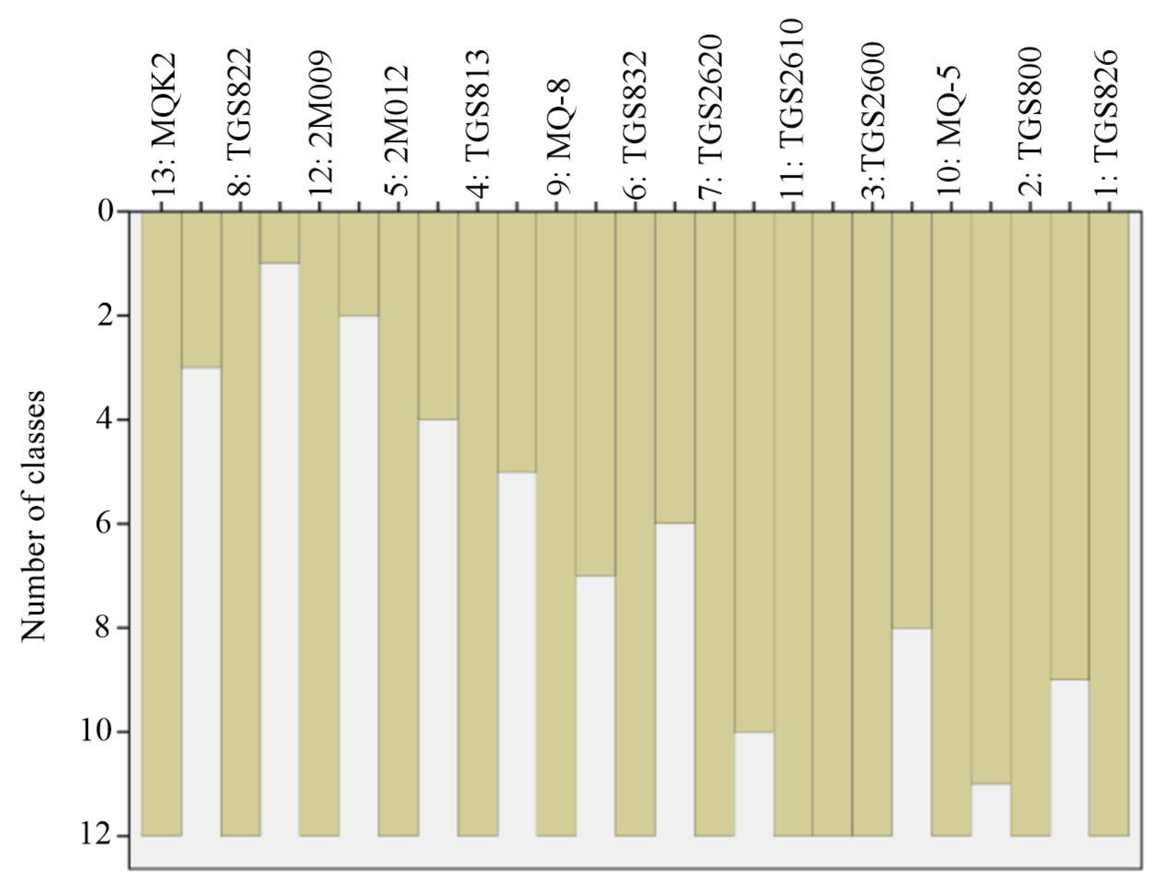
3.1.2. Optimization of Sensor Array LF for Fried Green Tea

Fried green tea accounts for approximately 70% of green tea in China. When LG is directly used to discriminate between varieties of fried green tea, the results are not quite satisfactory. Therefore, it is necessary to screen out the sensor array for fried green tea. Here, we specify that there are 8 sensors (N = 8) in sensor array LF, which is equal to that of LG. The fried green tea samples used for LF optimization are msqf, dgdf and qs.

According to the high correlated sensors listed in Table 3, we used the DPVs for 3 fried green teas that were listed in Table 4 to decide which sensor should be eliminated. For msqf, sensors of TGS822, TGS2620 and 2M009 should be eliminated; for dgdf, sensors of TGS826, TGS822, MQ-8 and TGS2620 should be eliminated; and for qs, sensors of TGS822, MQK2 and MQ-8 should be eliminated. Thus, TGS822, TGS2620 and MQ-8 were eliminated from LF since they were rejected by two or more kinds of green tea. After removal, the retained 12 sensors were 2M009, TGS813, TGS832, MQ-6, MQ-5, MQ-3, 2M012, TGS2600, TGS2610, TGS826, MQK2 and TGS800. Then, we took the average value of aroma data of each sensor to each sample of different kinds of fried tea as input for SPSS software, and produced and icicle figure of the clustering process, as shown in Figure 8. Similarly, we grouped the sensors into 8 classes, as described previously, namely TGS813, MQK2, MQ-6, 2M009, 2M012, (MQ-5/TGS832/TGS800), (MQ-3/TGS2600) and (TGS2610/TGS826). For each clustered sensor class, we selected a sensor with maximum DPV for 3 fried green teas, as listed in Table 4, and constructed an optimized sensor array LF with number N = 8, namely TGS813, MQK2, MQ-6, 2M009, 2M012, MQ-5, MQ-3 and TGS2610.

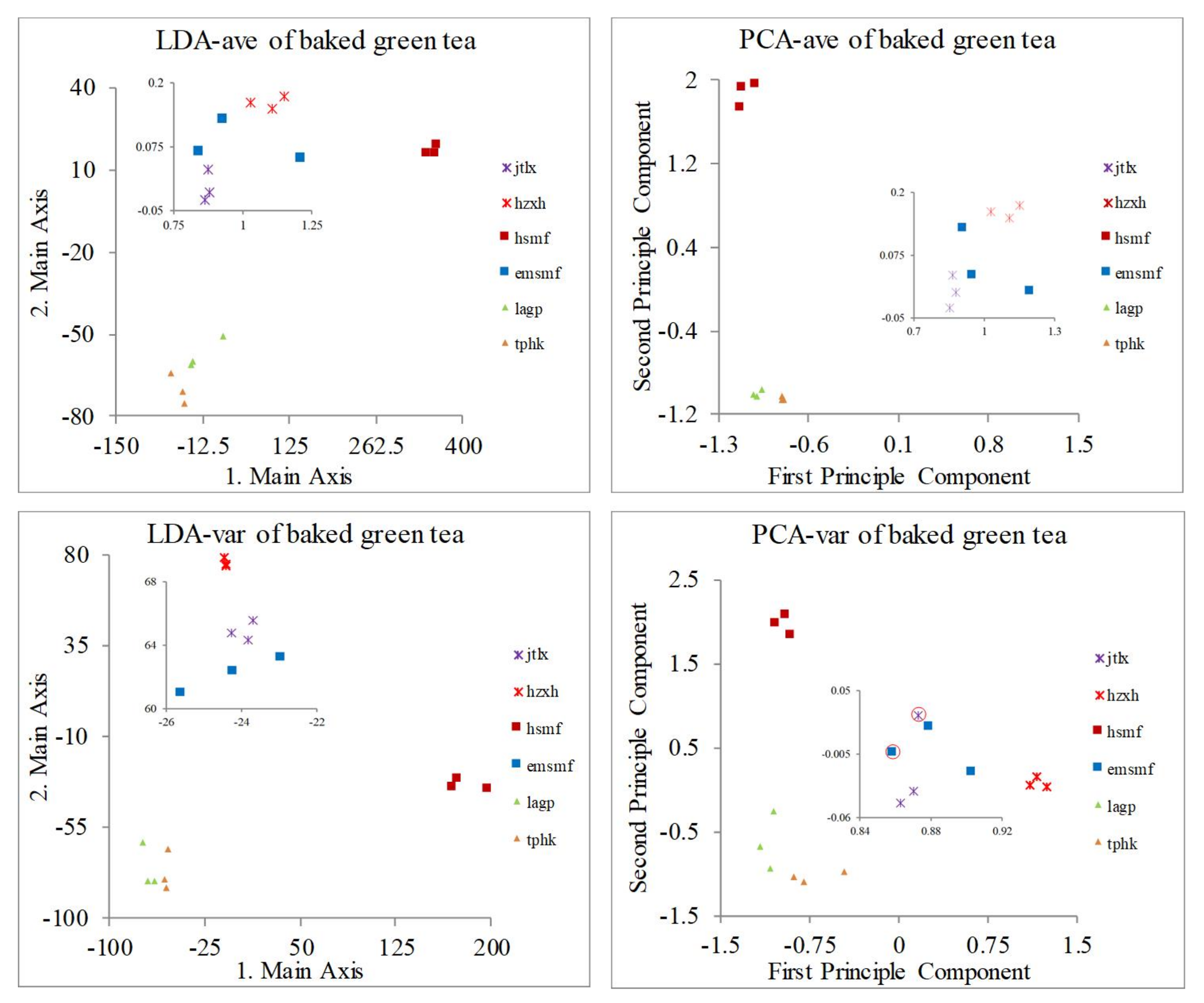
3.1.3. Optimization of Sensor Array LB for Baked Green Tea

Lagp, hsmf and tphk were used as baked green tea examples for the optimization of sensor array LB. Similarly, according to the high correlated sensors listed in Table 3, we used the DPVs for 3 kinds of baked green tea that were listed in Table 4 to decide which sensor should be eliminated. For lagp, sensors of 2M012 and MQ-3 should be eliminated; for hsmf, sensors of MQ-6 and MQ-5 should be eliminated; and for tphk, sensors of MQ-3 and MQ-6 should be eliminated. Thus, MQ-3 and MQ-6 were eliminated from LF since they were rejected by two or more kinds of green tea. After removal, the retained 13 sensors were TGS822, TGS813, 2M009, TGS832, TGS800, MQ-5, 2M012, TGS2620, TGS826, TGS2600, MQK2, MQ-8 and TGS2610.

Then, we took the average value of aroma response data of each sensor to each sample of different kinds of baked tea as input for SPSS software, and produced an icicle figure of the clustering process, as shown in Figure 9. Similarly, we grouped the sensors into 8 classes, as described previous, namely MQK2, TGS822, 2M009, 2M012, TGS813, MQ-8, TGS832 and (TGS2620/TGS2610/TGS2600/MQ-5/TGS800/TGS826). For each clustered sensor class, we selected a sensor with maximum DPV for 3 kinds of baked green tea, as listed in Table 4, and constructed an optimized sensor array LB with number N = 8, namely MQK2, TGS822, 2M009, 2M012, TGS813, MQ-8, TGS832 and TGS2620.

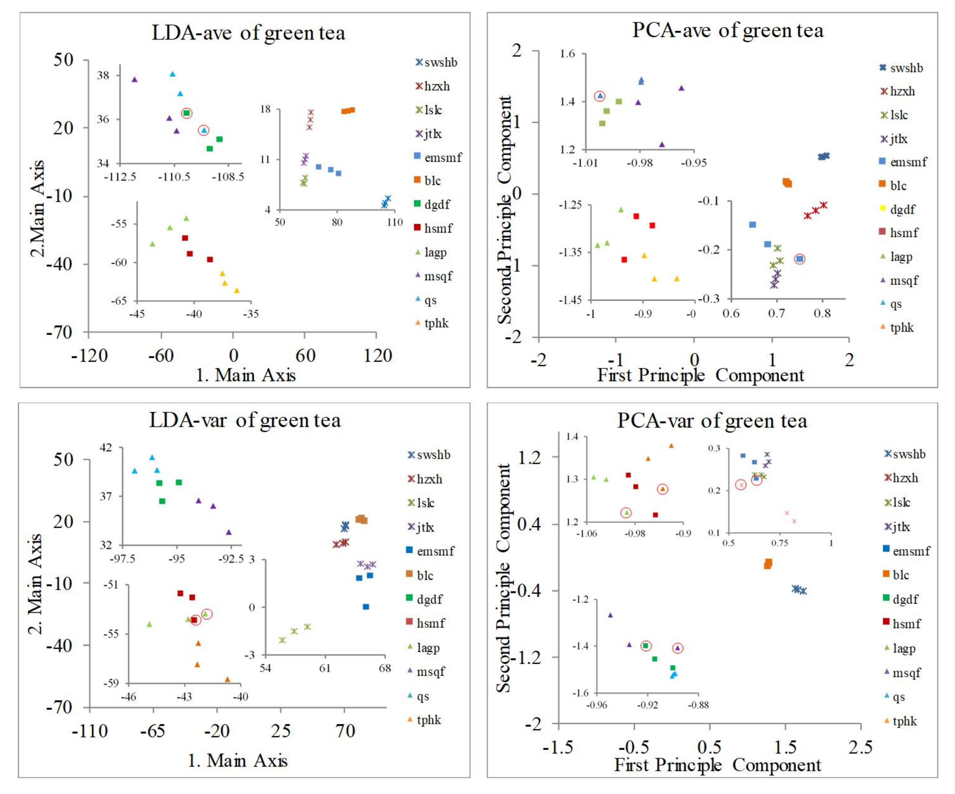
3.2. Classification of Green Tea Varieties

Three groups of optimized sensor arrays (LG, LF and LB) obtained for green tea, fried green tea and baked green tea, respectively, were generated based on the process above. The discriminating accuracy of these 3 sensor arrays needs to be further verified. The data analysis methods used were PCA based on the average value (PCA-ave), LDA based on the average value (LDA-ave), PCA based on the maximum variance moment (PCA-var) and LDA based on the maximum variance moment (LDA-var). Similar methods are also described in [30].

The results of the 12 varieties of green tea detected by sensor array LG are shown in Figure 10 and

Table 9. Discrimination accuracy of tea varieties by sensor array optimized for specific kinds of tea.

No. Tea Varieties	Sensor Array	LDA-ave	PCA-ave	LDA-var	PCA-var
12 kinds of green tea	LG	2 tea areas overlap (qs and dgdf)	2 tea areas overlap (lslc and emsmf)	2 tea areas overlap (lagp and hsmf)	4 tea areas overlap (msqf and dgdf, lslc and emsmf)
6 kinds of fried green tea	LF	100%	100%	2 tea areas overlap (dgdf and qs)	100%
6 kinds of baked green tea	LB	100%	100%	100%	2 tea areas overlap (emsmf and jtlx)
No. Tea Varieties	Sensor Array	LDA-ave +NNC	PCA-ave +NNC	LDA-var +NNC	PCA-var +NNC
12 kinds of green tea	LG	94.44%	94.44%	94.44%	83.33%
6 kinds of fried green tea	LF	100%	100%	88.89%	100%
6 kinds of baked green tea	LB	100%	94.44%	100%	88.89%

. There are 2, 2, 2 and 4 kinds of tea area overlap that occur in LDA-ave, PCA-ave, LDA-var and PCA-var, respectively. As shown in Figure 11 and Table 9, when discriminating between 6 varieties of fried green tea using LF, there are 2 kinds of tea area overlap occurring in LDA-var. For discriminating between 6 varieties of baked green tea using LB, there are 2 kinds of tea area overlap occurring in PCA-var, as shown in Figure 12 and Table 9. Because of the large degree of dispersion between inter-classes, the scale range of the whole graph is large, and the points of some regions appear to gather on the whole graph. As a result, some local magnifications are added to the whole graph to represent the local aggregation points. For easy understanding, the points of incorrect distinguished results are red-circled in Figure 10, Figure 11 and Figure 12.

In general, the discrimination accuracy of fried green tea by LF or baked green tea by LB is higher than that of general green tea by LG. It seems that there are some effects in SAO for green tea with specified processing techniques.

According to Figure 10, Figure 11 and Figure 12, we can see the distribution of dispersion and concentration of the discrimination results, and find out whether there are regional overlaps. However, in order to obtain the discrimination accuracy value, it is necessary to combine some classification algorithms. Here, we used NNC to obtain discrimination accuracy value, as shown in Table 9.

When LDA-ave +NNC are used, satisfactory results are obtained. The discrimination accuracy of LG for 12 kinds of green tea, LF for 6 kinds of faked green tea and LB for 6 kinds of baked green tea can almost reach to 88.89~100%.

Note that NNC may lead to misjudgments. For example, when detecting 12 kinds of green tea by LG and PCA-ave, a feature value of qs is misjudged as dgdf since they are closer to the center of dgdf, although qs and dgdf seem to be correctly separated, as shown in Figure 10. Similarly, a feature value of emsmf is misjudged as jtlx when detecting 6 baked green teas by LB and PCA-ave, as shown in Figure 12. These misjudgments will reduce the accuracy of tea discrimination.

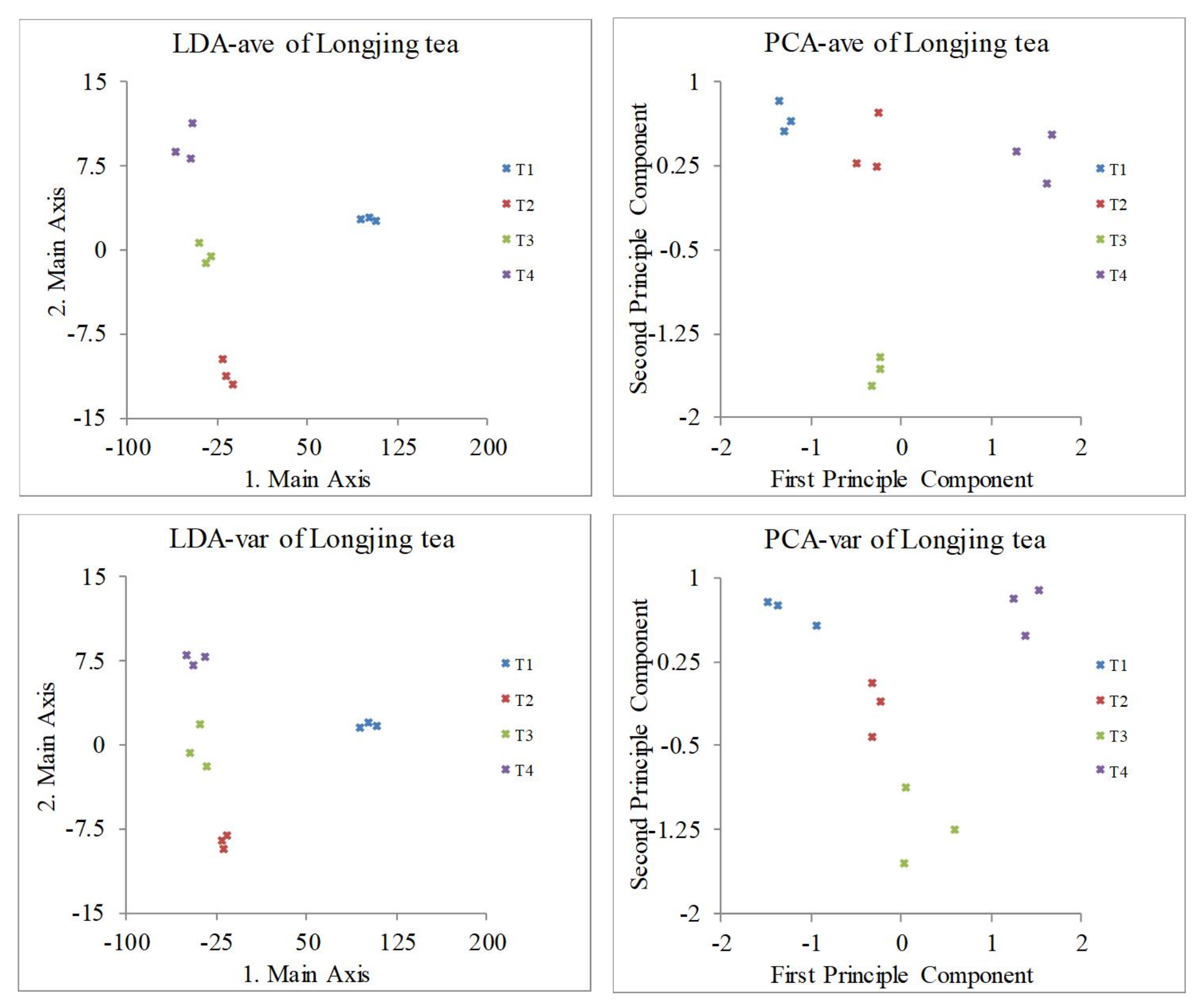
3.3. Classification of West Lake Longjing Tea Grade

Here, we further discriminated between different grades of identical fried green tea. Since West Lake Longjing is the most common representative of fried green tea, we will consider 4 grades of West Lake Longjing tea as examples.

It can be seen in Figure 13 and

Table 10. Discrimination accuracy of West Lake Longjing tea grades by LF.

Methods	LDA-ave (+NNC)	PCA-ave (+NNC)	LDA-var (+NNC)	PCA-var (+NNC)
LF	100%	100%	100%	100%

that the LDA-ave, PCA-ave and LDA-var methods all have good classification effects on West Lake Longjing tea using LF. Some scholars also used the commercial electronic nose PEN2 to carry out Longjing tea quality identification research [32]. Taking into account the difference between the experimental sample and the environment, it is not scientific to directly compare the two electronic noses quantitatively. However, it can be concluded that in the identification of Longjing tea grades, our self-made electronic nose using the optimized sensor array can achieve an effect comparable to that of the PEN2 electronic nose.

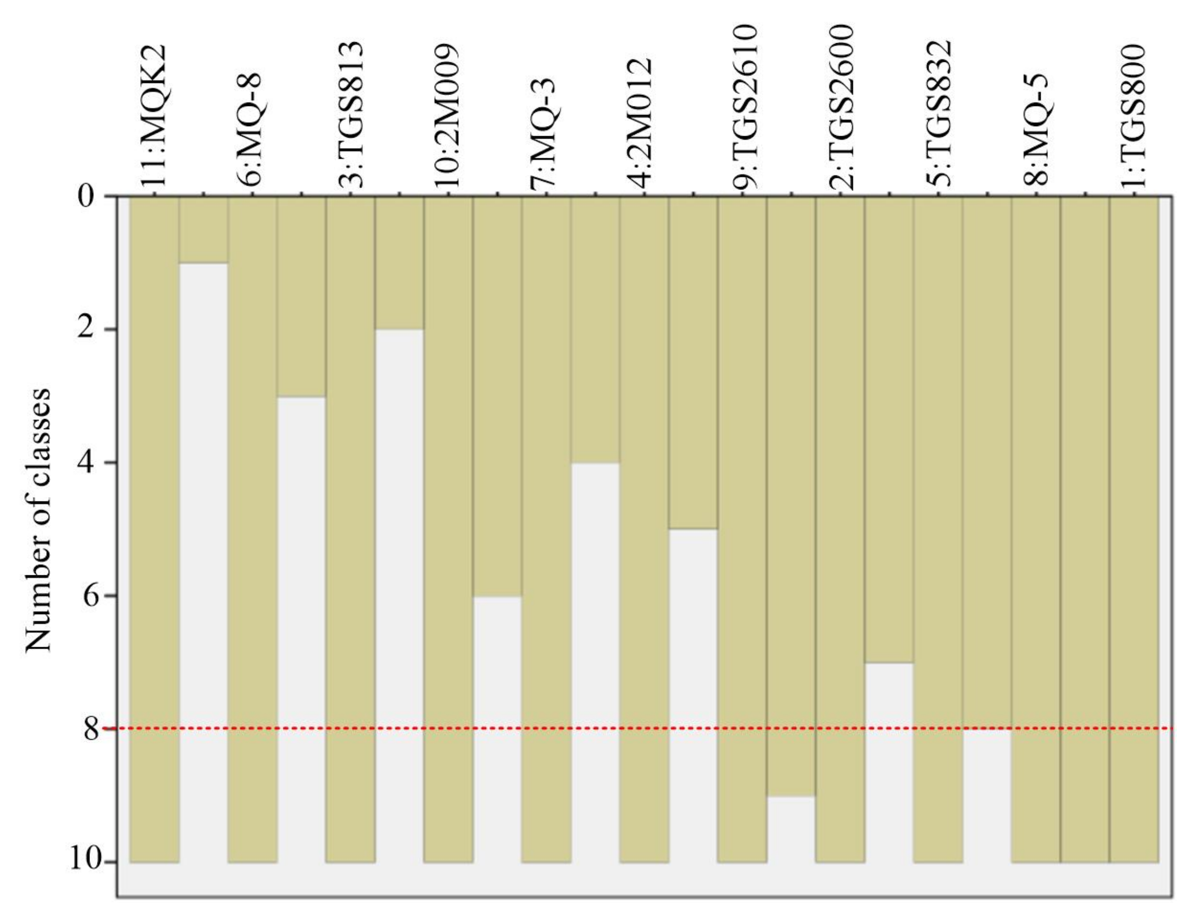
3.4. Comparison of Correlation Analysis Methods and the Elimination of Sensors

In this paper, we used DPVs to eliminate the correlated sensors; the principles and characteristics of these methods are listed in

Table 11. Comparison of correlated sensor analysis and elimination methods.

Method	Principle	Characteristics
Correlation analysis	$\left|R_{xy}\right|=\left|\frac{{\displaystyle {\sum }_{i=1}^N\left(x_i-\overline{x}\right)\left(y_i-\overline{y}\right)}}{\sqrt{{{\displaystyle {\sum }_{i=1}^N{\left(x_i-\overline{x}\right)}^2\left(y_i-\overline{y}\right)}}^2}}\right|$ The correlation calculation formula is identical to Formula (1) in this paper.	Calculate the sum of each sensor’s correlation coefficients and eliminate the sensor with the largest sum. Optimizes the correlation between sensors, but does not judge the discriminating ability of the sensor.
COV	$RSD=\frac{\sqrt{\frac{1}{n}{\displaystyle {\sum }_{i=1}^n{\left(x_i-\overline{x}\right)}^2}}}{\overline{x}}$ Where $x_i$ is the i-th test value of the gas sensor, $\overline{x}$ is the average value of the gas sensor at different times, and $n$ is the total number of tests.	The larger the coefficient of variation, the greater the intra-class dispersion of the sensor to detect the same class of tea. Therefore, sensors with large coefficients of variation were eliminated. This method does not judge the dispersion between classes and does not optimize the correlation between sensors.
DPV	$F_{\mathrm{i}}=\frac{\frac{1}{n}{\displaystyle {\sum }_{i=1}^n\left(u_i-u\right)}{\left(u_i-u\right)}^T}{\frac{1}{n}\times \frac{1}{m}{\displaystyle {\sum }_{i=1}^n{\displaystyle {\sum }_{k=1}^m\left(u_i-x_k\right){\left(u_i-x_k\right)}^T}}}$ The calculation formula for DPV is introduced in Equation (2) of this paper.	The DPV considers the inter- and intra-class dispersion of sensors. Optimizes sensors’ discriminating performances but does not optimize the correlation between sensors.

. Coefficient of variation (COV) is another common index that can reflect the dispersion degree of the observed values for each indicator on the unit mean. COV has also been introduced for the screening and elimination of sensors, which is compared with the method proposed in this paper.

In order to verify the classification effect of the sensor array obtained by different methods, we discriminated 6 tea samples for training using 6 group sensors: preliminary 15 sensors, 3 groups of random-selected 11 sensors, 11 sensors screened by correlation analysis and COV as well as 11 sensors screened by correlation analysis and the DPV. The discriminating results are shown in

Table 12. Discrimination accuracy of the sensors screened by different methods at the first step.

Sensor Screening Method	Selected Sensor Array	Discrimination Accuracy
		RFML [18]	LDA-ave	PCA-ave	LDA-var	PCA-var
Random selection 1	TGS826, TGS899, TGS2600, TGS813, 2M012, MQ6, TGS2620, TGS822, MQ3, 2M009, MQK2	97.81%	100.00%	72.22%	88.89%	66.67%
Random selection 2	TGS826, TGS899, TGS2600, TGS813, 2M012, MQ6, TGS2620, TGS822, MQ3, TGS2610, MQK2	98.15%	100.00%	72.22%	94.44%	66.67%
Random selection 3	TGS822, MQ5, TGS826, MQ6, 2M012, TGS2600, TGS2610, TGS800, 2M009, TGS2620, MQ3	96.05%	88.89%	61.11%	83.33%	77.78%
Preliminary sensors	TGS2600, TGS813, 2M012, MQ-6, TGS832, GS2620, MQ-8, MQ-3, MQ-5, TGS2610, 2M009, MQK2, TGS822, TGS826, TGS800	99.85%	100.00%	72.22%	100.00%	66.67%
Correlation analysis and COV	TGS2600, TGS813, 2M012, MQ-8, MQ-3, MQ5, TGS2610, 2M009, MQK2, TGS800, TGS826	98.33%	100.00%	66.67%	83.33%	72.22%
Correlation analysis and DPV	TGS800, TGS2600, TGS813, 2M012, TGS832, MQ-8, MQ-3, MQ-5, TGS2610, 2M009, MQK2	98.90%	100%	83.33%	94.44%	88.89%

. Sensors screened by the correlation analysis and the DPV have a better discrimination performance than that by the correlation analysis and COV, or by random. This is due to the fact that the DPV simultaneously considers the inter- and intra-class dispersion of sensors and is better for eliminating correlated sensors, which are analyzed using correlation analysis. The preliminary 15-sensor array combined with RFML has the highest accuracy. Sensors screened by the correlation analysis and the DPV have the most balanced performance. From the perspective of data processing efficiency and equipment cost, the 11-sensor array screened by the correlation analysis and the DPV is obviously better than the preliminary 15-sensor array.

3.5. Comparison of Screening Methods for Given Number of Sensors N

The second optimization step is to select N sensors from 11 sensors remained after the first step to construct a sensor array with good independence. For N = 8, the sensor array optimized by CA and DPV for 6 kinds of green tea is (MQK2, MQ-8, TGS813, 2M009, MQ-3, 2M012, TGS2600, TGS832), and the corresponding rankings of DPV are (2, 1, 6, 10, 3, 4, 11, 8). If the sensor array is optimized only by the ranking order of DPVs at the second step, the result is (MQ-8, MQK2, MQ-3, 2M012, TGS813, TGS832, 2M009, TGS2600), and the corresponding rankings of DPV are (1, 2, 3, 4, 6, 8, 10, 11). Note that two methods of CA + DPV and only DPV were used in selecting 8 sensors at the second optimization step, and the results are coincidentally consistent.

Thus, in order to show the effect of SAO at the second step, we constructed 5 sensor array groups. Four of them were randomly selected from the eleven sensors remained after the first step, and the other group was selected using CA and the DPV. The accuracy with which each of the 5 sensor groups were discriminated between 6 tea examples for training is shown in

Table 13. Discrimination accuracy of the different 8 sensors screened using different methods.

Sensor Screening Method	Selected Sensor Array	Discrimination Accuracy
		RFML [15]	LDA-ave	PCA-ave	LDA-var	PCA-var
Random selection-1	TGS832, MQ-8, MQ-3, MQ-5, TGS2610, 2M009,TGS2600, TGS813	96.60%	88.89%	83.33%	100%	88.89%
Random selection-2	MQ-8, MQ-3, MQ-5, TGS2610, 2M009, MQK2, TGS832, TGS813	97.26%	83.33%	83.33%	94.44%	77.78%
Random selection-3	MQ-8, MQ-3, MQ-5, TGS2610, 2M009, MQK2, TGS813, 2M012	97.64%	94.44%	77.78%	88.89%	66.67%
Random selection-4	TGS813, TGS2600, 2M012, MQ-3, 2M009, TGS800, MQ-5, TGS2610	83.08%	88.89%	77.78%	94.44%	83.33%
CA and DPV	MQK2, MQ-8, TGS813, 2M009, MQ-3, 2M012 TGS2600, TGS832	98.84%	88.89%	88.89%	100%	94.44%

. The results show that the sensor array selected using CA and DPV screening has almost the best performance in most cases, because the sensor array has better independence based on CA and better discrimination performance based on the DPV.

4. Conclusions

This paper proposed an optimization of an electronic nose sensor array to detect tea aroma based on correlation coefficient and cluster analysis. A method based on correlation coefficient and DPV is proposed to eliminate redundant sensors with high correlation coefficients. Three sensor arrays are constructed based on green tea (LG), fried green tea (LF) and baked green tea (LB), respectively. Based on the optimized sensor array LG, only 2 kinds of tea areas are overlapped when discriminating 12 green tea varieties by LDA-ave, LDA-var and PCA-ave methods. Combined with the NNC algorithm, the accuracy can reach 83.33–94.44%. This indicates that the tea aroma data obtained by LG have high quality. When detecting various grades of West Lake Longjing tea, LF shows comparable discrimination accuracy to that of the German PEN2 electronic nose based on the same data-processing method. Then, some sensor arrays screened and constructed based on other SAO methods were also experimented in the same electronic nose system for the identification of tea types. The experimental results show that sensors screened by the correlation analysis and the DPV have a better discrimination performance than that by the correlation analysis and COV, or by random. Finally, yet importantly, given the number of sensors, the proposed method can filter out the optimal sensor combination from the given candidate list.

The results show that, after proper optimization, fewer sensors can not only stop the reduction of the sensor array’s performance in tea aroma detection, but can also improve it; this is because, in our model, the introduction of noise is reduced. The electronic nose SAO method proposed in this paper can effectively eliminate redundant sensors and improve the quality of original tea aroma data. Fewer sensors also help simplify the circuit board design, provide a higher degree of freedom in the layout of system components and facilitate the miniaturization of the electronic nose system. In addition, fewer sensors can reduce the cost of the sensor array, which is beneficial to providing more design freedom for other modules in the system, thus having the potential to reduce system costs.

References

1. Ho, C.T.; Zheng, X.; Li, S. Tea aroma formation. Food Sci. Hum. Wellness 2015, 4, 9–27. [Google Scholar] [CrossRef] [Green Version]
2. Xia, T.; Shi, S.; Wan, X. Impact of ultrasonic-assisted extraction on the chemical and sensory quality of tea infusion. J. Food Eng. 2006, 74, 557–560. [Google Scholar] [CrossRef]
3. Qian, K.; Bao, Y.; Zhu, J.; Wang, J.; Wei, Z. Development of a portable electronic nose based on a hybrid filter-wrapper method for identifying the Chinese dry-cured ham of different grades. J. Food Eng. 2021, 290, 110250. [Google Scholar] [CrossRef]
4. Bhattacharyya, N.; Bandyopadhyay, R.; Bhuyan, M.; Tudu, B.; Ghosh, D.; Jana, A. Electronic nose for black tea classification and correlation of measurements with “Tea Taster” marks. IEEE Trans. Instrum. Meas. 2008, 57, 1313–1321. [Google Scholar] [CrossRef]
5. Demir, N.; Ferraz, A.C.O.; Sargent, S.A.; Balaban, M.O. Classification of impacted blueberries during storage using an electronic nose. J. Sci. Food Agric. 2011, 91, 1722–1727. [Google Scholar] [CrossRef] [PubMed]
6. Majchrzak, T.; Wojnowski, W.; Dymerski, T.; Gębicki, J.; Namieśnik, J. Electronic noses in classification and quality control of edible oils: A review. Food Chem. 2018, 246, 192–201. [Google Scholar] [CrossRef] [PubMed]
7. Infante, R.; Farcuh, M.; Meneses, C. Monitoring the sensorial quality and aroma through an electronic nose in peaches during cold storage. J. Sci. Food Agric. 2008, 88, 2073–2078. [Google Scholar] [CrossRef]
8. Chen, H.Z.; Zhang, M.; Bhandari, B.; Guo, Z. Evaluation of the freshness of fresh-cut green bell pepper (Capsicum annuum var. grossum) using electronic nose. LWT 2018, 87, 77–84. [Google Scholar] [CrossRef] [Green Version]
9. Śliwińska, M.; Wiśniewska, P.; Dymerski, T.; Wardencki, W.; Namieśnik, J. Application of electronic nose based on fast GC for authenticity assessment of Polish homemade liqueurs called nalewka. Food Anal. Method 2016, 9, 2670–2681. [Google Scholar] [CrossRef] [Green Version]
10. Chaparro-Torres, L.A.; Bueso, M.C.; Fernández-Trujillo, J.P. Aroma volatiles obtained at harvest by HS-SPME/GC-MS and INDEX/MS-E-nose fingerprint discriminate climacteric behaviour in melon fruit. J. Sci. Food Agric. 2016, 96, 2352–2365. [Google Scholar] [CrossRef]
11. Liu, L.; Li, X.; Li, Z.; Shi, Y. Application of Electronic Nose in Detection of Fresh Vegetables Freezing Time Considering Odor Identification Technology. Chem. Eng. Trans. 2018, 68, 265–270. [Google Scholar] [CrossRef]
12. Musatov, V.Y.; Sysoev, V.V.; Sommer, M.; Kiselev, I. Assessment of meat freshness with metal oxide sensor microarray electronic nose: A practical approach. Sens. Actuators B Chem. 2010, 144, 99–103. [Google Scholar] [CrossRef]
13. Gamboa, J.C.R.; da Silva, A.J.; de Andrade Lima, L.L.; Ferreira, T.A. Wine quality rapid detection using a compact electronic nose system: Application focused on spoilage thresholds by acetic acid. LWT 2019, 108, 377–384. [Google Scholar] [CrossRef] [Green Version]
14. Marek, G.; Dobrzański, B.; Oniszczuk, T.; Combrzyński, M.; Ćwikła, D.; Rusinek, R. Detection and differentiation of volatile compound profiles in roasted coffee arabica beans from different countries using an electronic nose and GC-MS. Sensors 2020, 20, 2124. [Google Scholar] [CrossRef]
15. Gonzalez Viejo, C.; Tongson, E.; Fuentes, S. Integrating a Low-Cost Electronic Nose and Machine Learning Modelling to Assess Coffee Aroma Profile and Intensity. Sensors 2021, 21, 2016. [Google Scholar] [CrossRef]
16. Rasekh, M.; Karami, H.; Wilson, A.D.; Gancarz, M. Performance Analysis of MAU-9 Electronic-Nose MOS Sensor Array Components and ANN Classification Methods for Discrimination of Herb and Fruit Essential Oils. Chemosensors 2021, 9, 243. [Google Scholar] [CrossRef]
17. Xu, M.; Wang, J.; Gu, S. Rapid identification of tea quality by E-nose and computer vision combining with a synergetic data fusion strategy. J. Food Eng. 2019, 241, 10–17. [Google Scholar] [CrossRef]
18. Lu, X.; Wang, J.; Lu, G.; Lin, B.; Chang, M.; He, W. Quality level identification of West Lake Longjing green tea using electronic nose. Sens. Actuators B Chem. 2019, 301, 127056. [Google Scholar] [CrossRef]
19. Yu, H.; Wang, J.; Yao, C.; Zhang, H.; Yu, Y. Quality grade identification of green tea using E-nose by CA and ANN. LWT—Food Sci. Technol. 2008, 41, 1268–1273. [Google Scholar] [CrossRef]
20. Zhu, J.; Chen, F.; Wang, L.; Niu, Y.; Xiao, Z. Evaluation of the synergism among volatile compounds in Oolong tea infusion by odour threshold with sensory analysis and E-nose. Food Chem. 2017, 221, 1484–1490. [Google Scholar] [CrossRef]
21. Yu, H.; Wang, J. Discrimination of LongJing green-tea grade by electronic nose. Sens. Actuators B Chem. 2007, 122, 134–140. [Google Scholar] [CrossRef]
22. Yu, H.; Wang, J.; Xiao, H.; Liu, M. Quality grade identification of green tea using the eigenvalues of PCA based on the E-nose signals. Sens. Actuators B Chem. 2009, 140, 378–382. [Google Scholar] [CrossRef]
23. Men, H.; Fu, S.; Yang, J.; Cheng, M.; Shi, Y.; Liu, J. Comparison of SVM, RF and ELM on an Electronic Nose for the Intelligent Evaluation of Paraffin Samples. Sensors 2018, 18, 285. [Google Scholar] [CrossRef] [PubMed] [Green Version]
24. Xu, L.; Yu, X.; Liu, L.; Zhang, R. A novel method for qualitative analysis of edible oil oxidation using an electronic nose. Food Chem. 2016, 202, 229–235. [Google Scholar] [CrossRef]
25. Yin, Y.; Hao, Y.; Yu, H. Identification method for different moldy degrees of maize using electronic nose coupled with multi-features fusion. Trans. Chin. Soc. Agric. Eng. 2016, 32, 254–260. [Google Scholar]
26. Yu, H.; Chu, B.; Yin, Y. Evaluation method of feature vector in vinegar identification by electronic nose. Trans. Chin. Soc. Agric. Eng. 2013, 29, 258–264. [Google Scholar]
27. Zhi, R.; Zhao, L.; Zhang, D. A framework for the multi-level fusion of electronic nose and electronic tongue for tea quality assessment. Sensors 2017, 17, 1007. [Google Scholar] [CrossRef] [PubMed] [Green Version]
28. Banerjee, M.B.; Roy, R.B.; Tudu, B.; Bandyopadhyay, R.; Bhattacharyya, N. Black tea classification employing feature fusion of E-Nose and E-Tongue responses. J. Food Eng. 2019, 244, 55–63. [Google Scholar] [CrossRef]
29. Zhang, L.; Tian, F. Performance study of multilayer perceptrons in a low-cost electronic nose. IEEE Trans. Instrum. Meas. 2014, 63, 1670–1679. [Google Scholar] [CrossRef]
30. Makimori, G.Y.F.; Bona, E. Commercial instant coffee classification using an electronic nose in tandem with the ComDim-LDA approach. Food Anal. Methods 2019, 12, 1067–1076. [Google Scholar] [CrossRef]
31. Yin, Y.; Zhao, Y. A feature selection strategy of E-nose data based on PCA coupled with Wilks Λ-statistic for discrimination of vinegar samples. J. Food Meas. Charact. 2019, 13, 2406–2416. [Google Scholar] [CrossRef]
32. Pardo, M.; Sberveglieri, G. Classification of electronic nose data with support vector machines. Sens. Actuators B Chem. 2005, 107, 730–737. [Google Scholar] [CrossRef]
33. Tan, J.; Kerr, W.L. Determining degree of roasting in cocoa beans by artificial neural network (ANN)-based electronic nose system and gas chromatography/mass spectrometry (GC/MS). J. Sci. Food Agric. 2018, 98, 3851–3859. [Google Scholar] [CrossRef]
34. Wijaya, D.R.; Afianti, F. Stability assessment of feature selection algorithms on homogeneous datasets: A study for sensor array optimization problem. IEEE Access 2020, 8, 33944–33953. [Google Scholar] [CrossRef]
35. Chen, R.R.; Luo, D.H.; Sun, Y.; Sun, Y.L.; Gholam Hossini, H. A Sensor Array Optimization Method Based on Variance Difference for Machine Olfaction. In Applied Mechanics and Materials; Trans Tech Publications Ltd.: Freinbach, Switzerland, 2014; Volume 618, pp. 523–527. [Google Scholar] [CrossRef]
36. Zhou, H.T.; Yin, Y.; Yu, H.C. Optimization method of gas sensor array for identification of Jing Wine based on electronic nose. Chin. J. Sens. Actuators 2009, 22, 175–178, (In Chinese with English abstract). [Google Scholar]
Figure 1. Response curves of sensors to West Lake Longjing tea. The dotted box contains stable data.
Chemosensors 09 00266 g001
Figure 2. Circuit schematic of TGS826 referred from product manual of Figaro Ltd.
Chemosensors 09 00266 g002
Figure 3. The internal structure and airflow of electronic nose system.
Chemosensors 09 00266 g003
Figure 4. Sensor array schematic and appearance.
Chemosensors 09 00266 g004
Figure 5. The overall appearance of the electronic nose system.
Chemosensors 09 00266 g005
Figure 6. The flow chart of the sensor array optimization method.
Chemosensors 09 00266 g006
Figure 7. Icicle figure of clustering sensors’ response average value (6 kinds of green tea).
Chemosensors 09 00266 g007
Figure 8. Icicle figure of clustering sensors’ response average value (3 kinds of fried green tea).
Chemosensors 09 00266 g008
Figure 9. Icicle figure of clustering sensors’ response average value (3 kinds of baked green tea).
Chemosensors 09 00266 g009
Figure 10. Classification results of green tea identified using LG.
Chemosensors 09 00266 g010
Figure 11. Classification results of fried green tea identified using LF.
Chemosensors 09 00266 g011
Figure 12. Classification results of baked green tea identified using LB.
Chemosensors 09 00266 g012
Figure 13. Grade classification results for West Lake Longjing tea identified using LF.
Chemosensors 09 00266 g013