Article

Origin Identification of Table Salt Using Flame Atomic Absorption and Portable Near-Infrared Spectrometries

by
Larissa Rodrigues Zanela Lima
1,
Luana Dalagrana dos Santos
1,
Isabella Taglieri
2,3,
David Cabral
2,
Letícia Estevinho
2,
Fábio Luiz Melquiades
4,
Luís Guimarães Dias
2,* and
Evandro Bona
1,2,5,*
1
Post-Graduation Program of Food Technology (PPGTA), Federal University of Technology Paraná (UTFPR), Campo Mourão 87301-899, Brazil
2
Centro de Investigação de Montanha (CIMO), Instituto Politécnico de Bragança, 5300-253 Bragança, Portugal
3
Department of Agriculture Food Environment, Interdepartmental Research Center, Nutraceuticals and Food for Health, University of Pisa, 56124 Pisa, Italy
4
Applied Nuclear Physics Laboratory, State University of Londrina (UEL), Londrina 86057-970, Brazil
5
Post-Graduation Program of Chemistry (PPGQ), Federal University of Technology Paraná (UTFPR), Curitiba 80230-901, Brazil
*
Authors to whom correspondence should be addressed.
Chemosensors 2025, 13(7), 231; https://doi.org/10.3390/chemosensors13070231
Submission received: 23 April 2025 / Revised: 18 June 2025 / Accepted: 19 June 2025 / Published: 24 June 2025
(This article belongs to the Special Issue Chemometrics Tools Used in Chemical Detection and Analysis)

Abstract

The mineral composition of table salt can be indicative of its origin. This work evaluated the possibility of identifying the origin of salt from four countries: Brazil, Spain, France, and Portugal. Eight metals were quantified through flame atomic absorption/emission spectroscopy (FAAS). The possibility of using portable near-infrared spectroscopy (NIR) as a faster and lower-cost alternative for identifying salt provenance was also evaluated. The content of Ca, Mg, Fe, Mn, and Cu was identified as possible markers to differentiate the salt origin. One-class classifiers using FAAS data and DD-SIMCA could discriminate the salt origin with few misclassifications. For NIR spectroscopy, it was possible to highlight the importance of controlling the humidity and granulometry before the spectra acquisition. After drying and milling the samples, it was possible to discriminate between samples based on the interaction between the water of hydration and the presence of the cations in the sample. The Mg, Mn, and Cu are important in identifying the origin of salt using NIR spectra. The DD-SIMCA model using NIR spectra could classify the origin with the same performance as observed in FAAS. However, it is important to emphasize that NIR spectroscopy requires less sample preparation, is faster, and has low-cost instrumentation.

Graphical Abstract

1. Introduction

Table salt, mainly composed of sodium chloride (NaCl), is widely used as a seasoning and preservative worldwide. Different table salt types are available: refined salt, sea salt, pink or Himalayan salt, flower salt, and light salt [1,2,3]. Iodine is sometimes added to salt as potassium iodide (KI) or potassium iodate (KIO3) to decrease the deficiency in the human diet [4]. Depending on the manufacturing process, other compounds were also found, like magnesium and calcium sulfates, carbonates, and chlorides [2,3]. The geographic origin of the salt also influences its mineral profile; for example, Atlantic and Mediterranean salt have different compositions regarding calcium, magnesium, and potassium [3]. The mineral profile can give different properties to table salt, adding value to the product, so it is important to guarantee traceability. Recent fraud scandals and food safety incidents have increased interest in food traceability. Food fraud leads to economic losses and the deterioration of the consumer’s trust, and it can also threaten human health. Therefore, more consumers want more detailed information about their foods, such as geographical origin, species, and transport and storage conditions [5]. Considering these facts, the elemental composition of the table salt could be used as a fingerprint to identify the salt’s origin.
Atomic spectroscopy is a consolidated methodology for elemental analysis [6]. Although this method requires time-consuming sample preparation, it demands expert analysts and high-cost instrumentation. Therefore, alternatives such as X-ray fluorescence [2] and near-infrared spectroscopy (NIR) [3,7] were already applied for salt analysis. NIR spectroscopy, which requires few sample preparation steps, is commonly applied in food authenticity and origin identification [8,9,10]. Furthermore, low-cost portable spectrometers are available for NIR spectroscopy, allowing this analysis to be applied to different foods [11,12]. NIR is a vibrational spectroscopy, but some authors demonstrate that metals could be indirectly identified and quantified due to the changes in the shape and peak position of the water peaks in the NIR spectrum. The extent of these changes depends on properties such as size and ionic strength, and this effect is also known as aquaphotomics [7,13,14]. The aquaphotomic effect allows the NIR spectra to quantify analytes in very low concentrations [14]. Despite the advantages already mentioned, NIR spectroscopy generates complex signals that require the application of chemometric methods to interpret the results [15]. Models based on discriminant analysis are the typical approach for dealing with authentication problems [16]. However, some authors argued that discriminant analysis is inappropriate and that the best approach is one-class classifiers (OCC) [17,18]. These methods distinguish objects of one particular class from all other classes [19]. The data-driven soft independent modeling by class analogy (DD-SIMCA) consists of a PCA model and an estimation of the orthogonal and score distances and their cut-off levels [20].
This work aimed to identify the origin of table salt from four countries by applying flame atomic absorption and near-infrared spectroscopies. The data collected by these two spectroscopies generated DD-SIMCA models to distinguish the table salt from different countries. The objective is to verify whether NIR spectra are sufficient to produce models to identify table salt’s origin. Therefore, this is the first work that applies NIR spectra in tandem with DD-SIMCA to classify the origin of table salt.

2. Materials and Methods

2.1. Samples

Fifty-nine salt samples bought in local markets were analyzed: 11 from Brazil (Figure S1—Supplementary Materials), 16 from Spain (Figure S2), 16 from France (Figure S3), and 16 from Portugal (Figure S4). The samples had different colors, humidity levels, and granulometry. Different types of salt were analyzed (label information), including flower salt, refined salt with or without iodine, sea salt, and light salt (sodium chloride was partially substituted by potassium chloride; SB1, SB2, SB3, and SF11). Therefore, the sample set has many different characteristics, and it was chosen to assess whether it is possible to identify the country of origin, even with these variations.

2.2. Humidity Analysis

The humidity was determined by weighing 10 g of the sample into a previously tared porcelain capsule. Heated for 3 h in an oven at 105 °C, cooled in a desiccator to room temperature, and weighed again. This procedure was repeated until a constant weight was achieved [21].

2.3. Flame Atomic Absorption/Emission Spectrometry Analysis

Potassium, sodium, calcium, magnesium, iron, manganese, zinc, and copper content in the salt samples was carried out in a flame atomic absorption spectrophotometer equipped with hollow cathode lamps (Perkin Elmer, model PinAAcle 900T, Waltham, MA, USA). For each element, the parameters and experimental conditions employed (wavelength, bandwidth, electric current, and gas flow rates) were set as recommended by the manufacturer.
About 0.05 g of salt was dissolved in 50 mL of HNO3 (2%) to determine K, Na, and Ca. Nearby, 0.50 g of salt was dissolved in 25 mL of HNO3 (2%) to determine Fe, Mn, Cu, Mg, and Zn. CsCl was added to the sample to determine K and Na, guaranteeing a final concentration of 1.0 g L−1. LaCl3 (1.0 g L−1) was added to the sample before determining Ca and Mg.
All standard solutions for the calibration curves were prepared from commercial solutions (1000 ppm) of different metals (Panreac, Darmstadt, Germany) diluted with HNO3 (5%). The concentration range of the calibration curves was 0.25 to 5.00 ppm for K, Ca, and Fe; 0.13 to 2.50 ppm for Na; 0.12 to 1.25 ppm for Mg; 0.12 to 4.00 ppm for Mn; 0.13 to 2.00 ppm for Cu; and 0.05 to 1.00 ppm for Zn. When necessary, samples were diluted to bring the concentration closer to the center of the calibration curve.

2.4. Near-Infrared Spectrometry Analysis

All spectra were obtained in the DLP NIRscan Nano evaluation module (Texas Instruments, Dallas, TX, USA). The DLP NIRscan Nano GUI was used to control the spectrometer and collect the spectra in reflectance mode. The scan configuration used was the Hadamard method, with a range of 900–1600 nm, a width of 4.68 nm, a digital resolution of 530 points, and an exposure time of 0.635 ms, resulting in a total scan time of ~17 s. The salt samples were put in polyethylene bags and analyzed in three different forms to evaluate the influence of granulometry and humidity in the spectra: (i) raw salt; (ii) dried salt (the samples were kept in an oven at 105 °C for 24 h); and (iii) dried-milled salt (after dried, the salt was milled in tube-mill (IKA, Staufen, Germany) at 10000 rpm for 1 min and then sieved using a 100 mesh nylon cloth). The spectra acquisition was repeated three times for each sample; the plastic bags containing the sample were shaken between acquisitions. After the acquisition, the spectra were transferred to MATLAB R2024b (MathWorks, Natick, MA, USA), smoothed with a cubic smoothing spline (smoothing parameter 0.005). The first derivative was determined using the central finite-difference method (CFDM). The objective of the first derivative is to eliminate the shift in the baseline, which is common in reflectance spectra obtained from powdered samples. For the data analysis step, the mean spectra were used.

2.5. Data Analysis

A one-way ANOVA was applied to assess whether there were significant differences between the mean results of the metal profile. In cases with p-value < 0.05, Tukey’s test checked the equality of means of two independent samples. When comparing medians, Wilcoxon’s rank sum test, a nonparametric test, was used. Samples with significant differences (p-value < 0.05) were represented with different letters.
The metals’ data were determined using FAAS, and the first derivative of the NIR spectra was used for unsupervised exploration using principal component analysis (PCA). For the PCA, all wavelengths of the first derivative of NIR spectra were considered (900–1600 nm, resolution ~2 nm), and the matrix was mean-centered before analysis. The salt classification was performed using DD-SIMCA with a rigorous approach to defining the number of PCS, chi-square acceptance area, classic method, and α = 0.05. The FAAS data were mean-centered and scaled, and the first derivative of the NIR spectra was mean-centered before DD-SIMCA modeling. We recommend reading the specialized literature for more information about the DD-SIMCA parameters [22]. All data analysis was made in MATLAB R2024b, and for DD-SIMCA, a graphical user interface (GUI) was used [19].

3. Results and Discussion
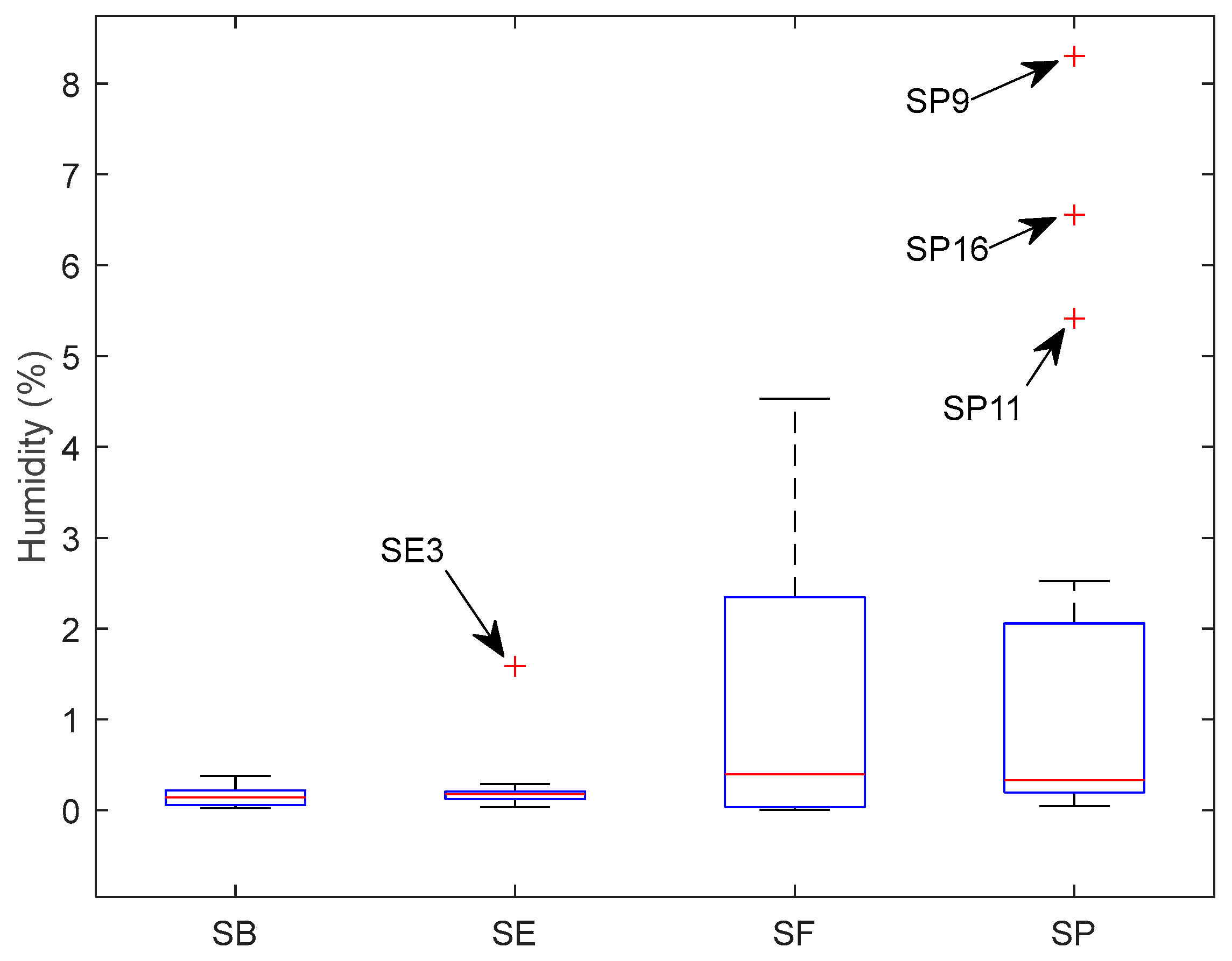
3.1. Humidity

The humidity for each sample is presented in the Supplementary Material (Table S1). Figure 1 shows the box plot to resume humidity variation in the samples for each country. Brazilian salt (SB) and Spain salt (SE) had less variation in humidity than France’s salt (SF) and Portugal’s salt (SP). The median is 0.1444% for SB, 0.1790% for SE, 0.3938% for SF, and 0.3343% for SP. SE had one sample with abnormally high humidity, and SP had three with higher humidity. These three SP samples were flower salt.

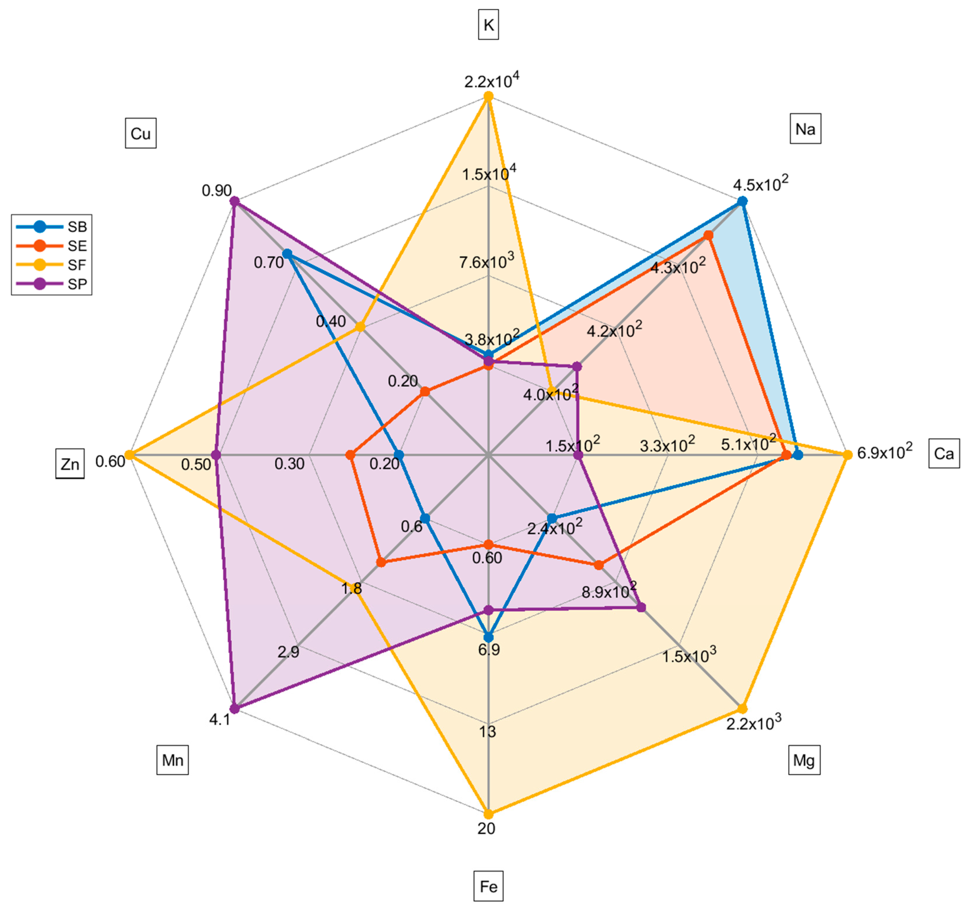
3.2. Flame Atomic Absorption/Emission Spectrometry

The table with eight metals quantified for each sample with FAAS is shown in the Supplementary Material (Table S2). Table 1 presents some descriptive statistics for each metal and country. The high variability for metal content for all countries stands out, as seen in the standard deviation values, variation range, and the difference between the mean and median. Only for potassium and sodium, statistically significant differences (p > 0.05) were not observed between the means of the countries. The sample SF11 (light salt) had an exceptionally high potassium content (about 81 times higher than the SB2, the second sample with the highest potassium content). The potassium concentration determined by FAAS to SF11 followed the potassium content declared in the salt package. The values obtained for the metal profile followed other consulted works [1,2,3].
In Figure 2, the radar plot highlights each country’s metal profile differences. The radar plot indicates that SP generally has a higher content of Cu and Mn and a lower content of Ca than other countries. SF has a higher content of Mg, Fe, and K. However, it is important to highlight the abnormal content of K in sample SF11 (Table S2, Supplementary Material), which raises the mean for France’s salt. Therefore, these differences must be carefully evaluated due to the high variation in the content of metals within samples from the same country.
The autoscaled matrix of the metal content in salt samples was submitted to the PCA. The scree and Pareto plots show that the first four principal components (PC) contributed most to representing the mineral content data (Supplementary Material—Figure S5). Furthermore, according to Figure S5c, PC5 has some information about Mg and PC6 about Zn. Nevertheless, looking at the scores plot for these PCs, there is no relevant separation for the samples, so they were not considered in the analysis. The first four PCs accumulated 79.3% of the total variance, with 34.9% in PC1, 18.6% in PC2, 16.8% in PC3, and 9.0% in PC4. Figure 3 resumes the PCA results obtained for metal content. All samples SE (except SE9) and SB (except SB2) had negative scores for PC1 (Figure 3a). The loadings (Figure 3b) indicate the highest positive weights for Zn, Fe, Mg, and Mn. So, the SE and SB samples have the lowest average contents for these salts, except for iron in the SB samples (see radar plot—Figure 2). In PC2, almost all SP samples had positive scores, while SB, SE, and SF had negative scores. The positive loading (Figure 3c) for the Cu content (highest mean value for SP) and K content (highest mean value for SF) was the main factor for this separation. In PC3, the SP samples had negative scores due to the lowest calcium content compared to other countries. The PC4 represents the difference in potassium content, and the light salt samples had positive scores. In Figure 3, it is possible to observe that some samples separated from the other salts. SF11, as mentioned before, had the highest level of potassium. SF12 had the highest level of magnesium. The light salt from Brazil was separated from other samples from this country due to its potassium content.
The DD-SIMCA [19] was employed to build OCC models for the metal content matrix, and the acceptance plots for each country are presented in Figure 4. In the acceptance plot, each sample is plotted using the score distance (h) and the orthogonal distance (v). The values h0 and v0 are scaling factors found during the model calibration step [22]. The autoscaled matrix was used for all OCC models due to the difference in the scale observed for the metal content matrix. In each model, the smallest number of PCs was used to allow adequate separation of the samples. For SB salt (Figure 4a,b), two samples of SE were misclassified (100% sensitive and 95.8% specific). For SE, one false negative was observed, and two samples of SB were misclassified (93.8% sensitive and 95.3% specific); for SF, two samples of SB were misclassified (100% sensitive and 95.3% specific); and for SP, one sample of SE was misclassified (100% sensitive and 97.8% specific). Considering the samples’ variability, the OCC models achieved good performance (seven false positives and one false negative). Therefore, the metal content could be used as a fingerprint to identify the country of origin for salt samples.

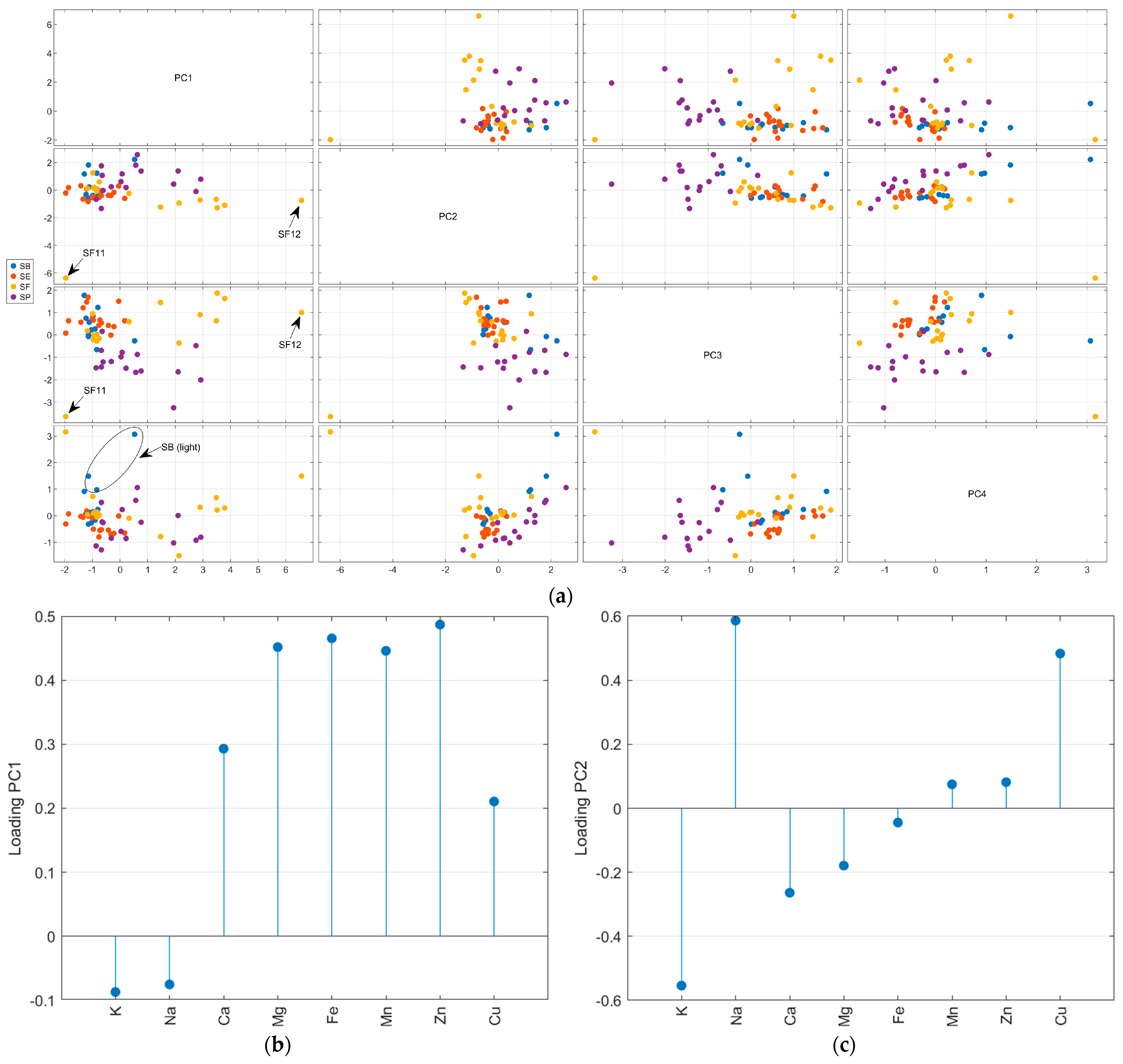
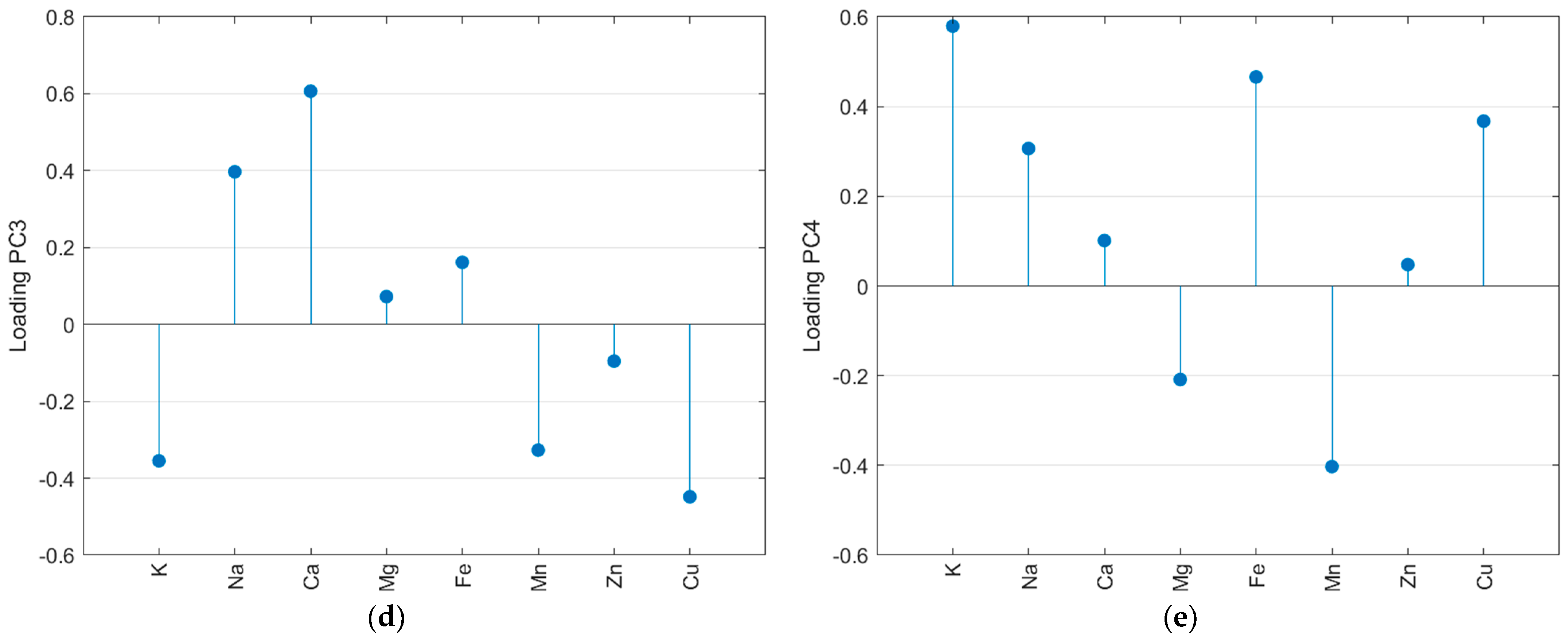
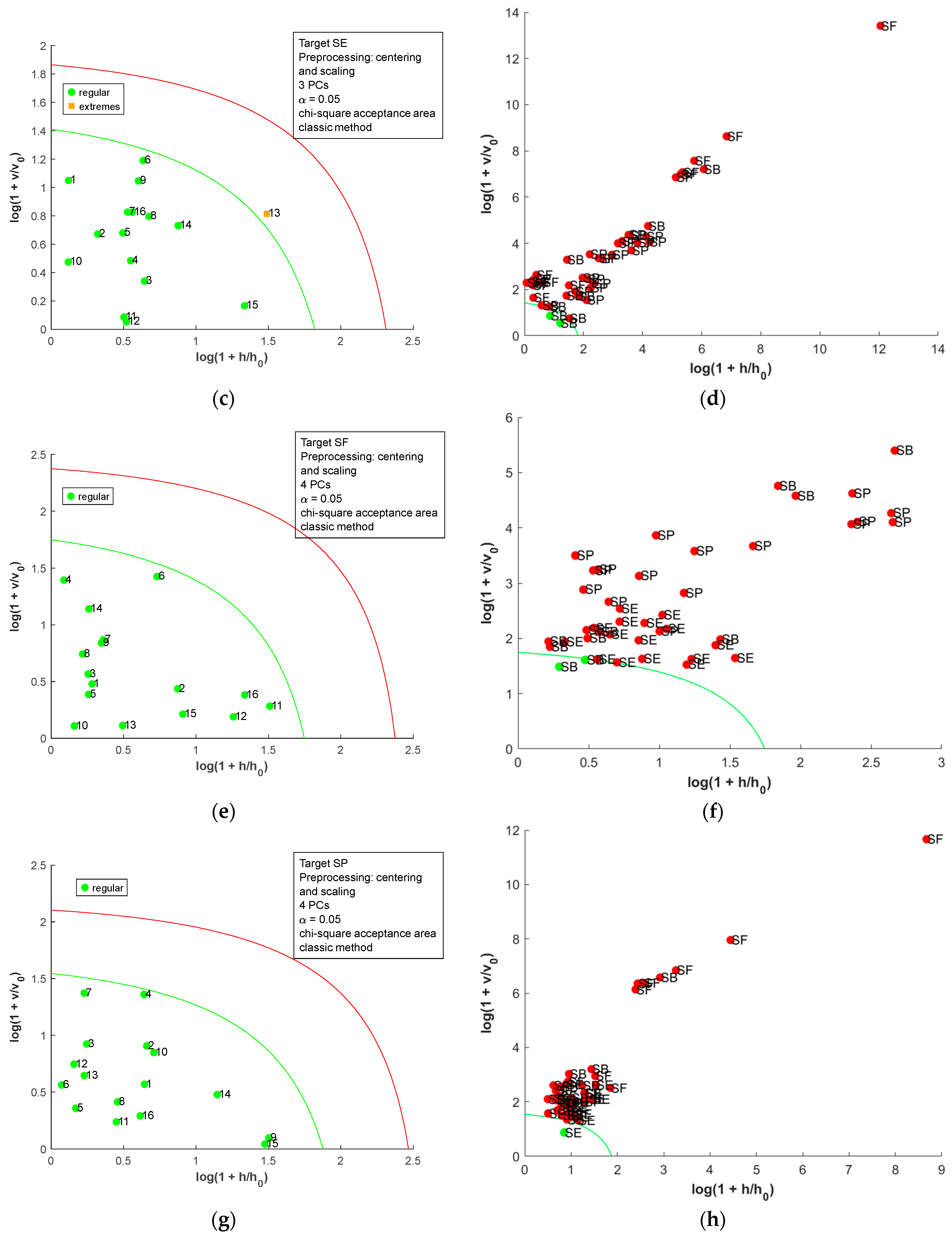
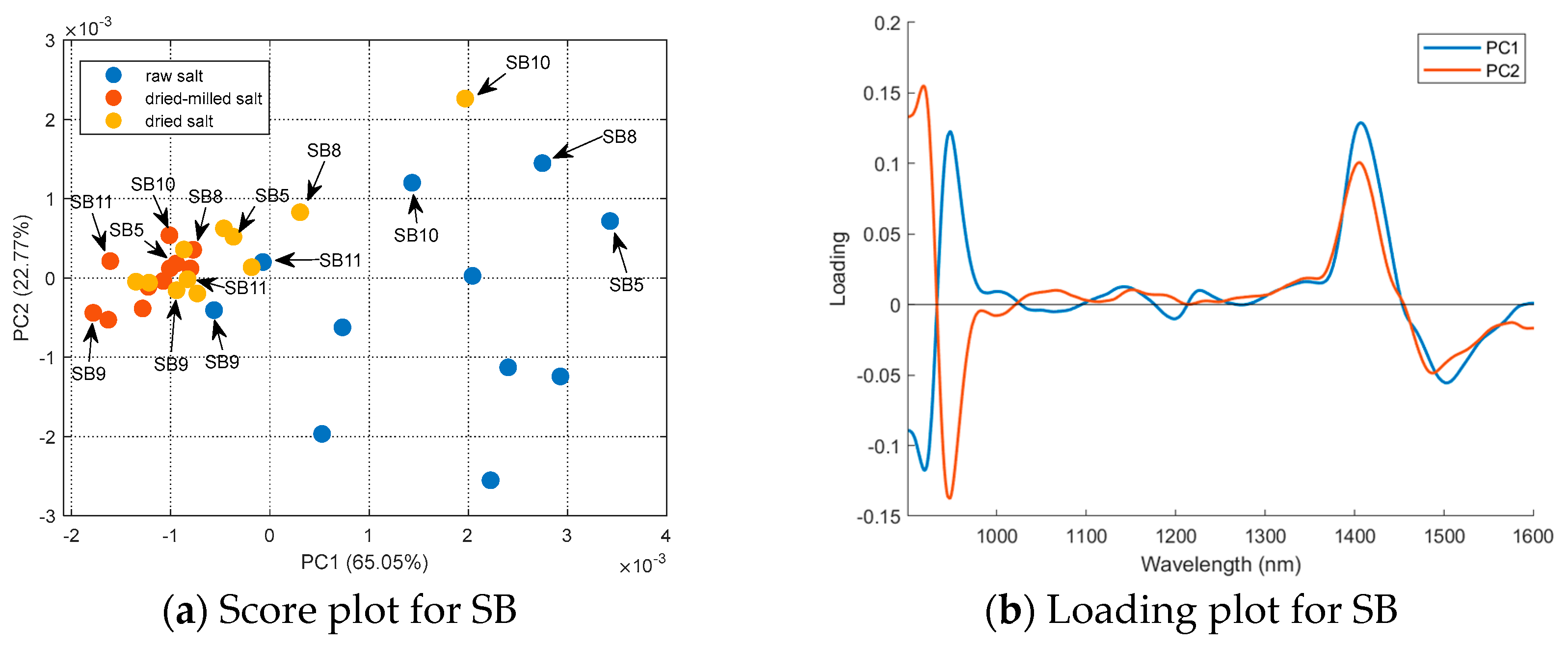
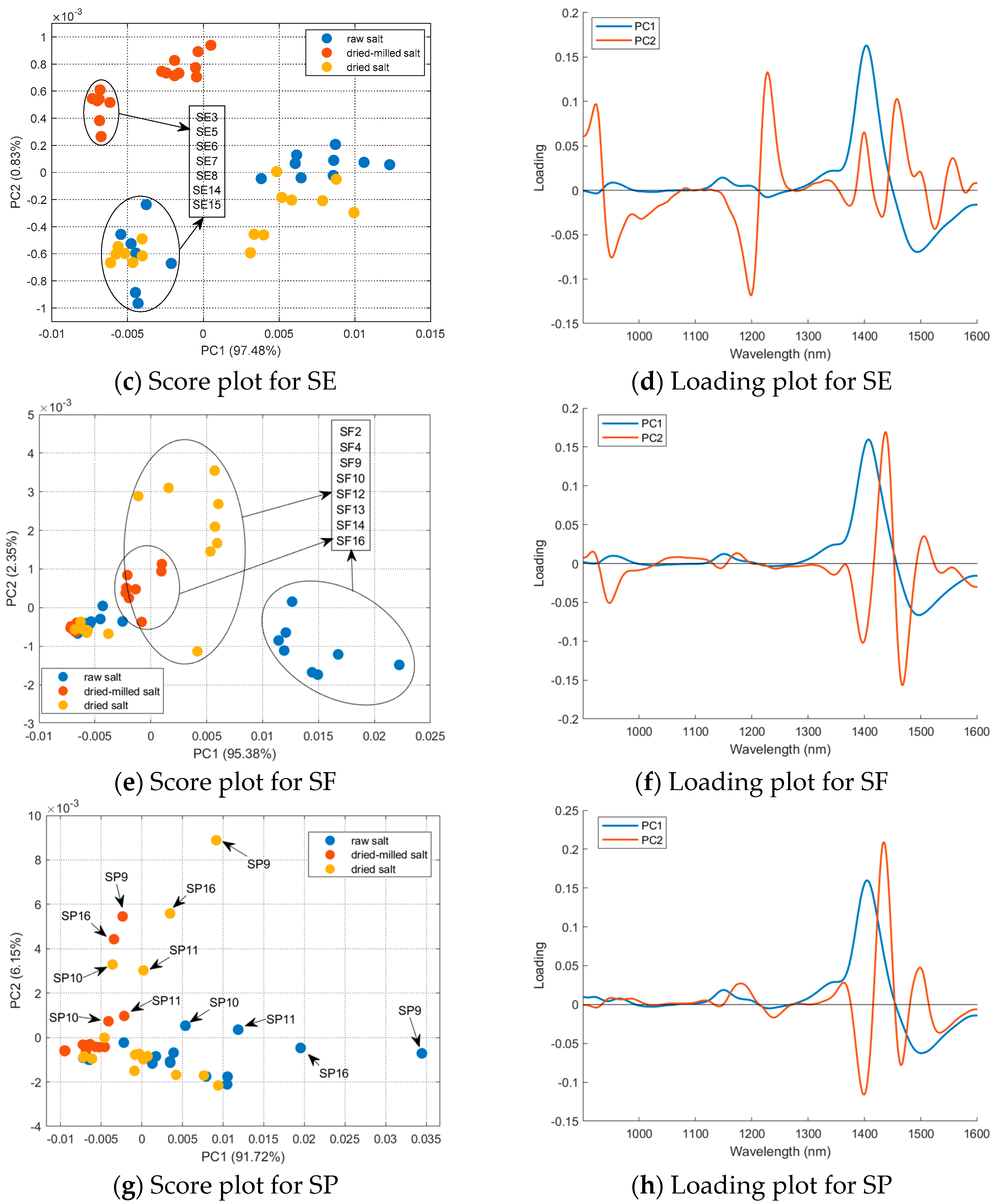
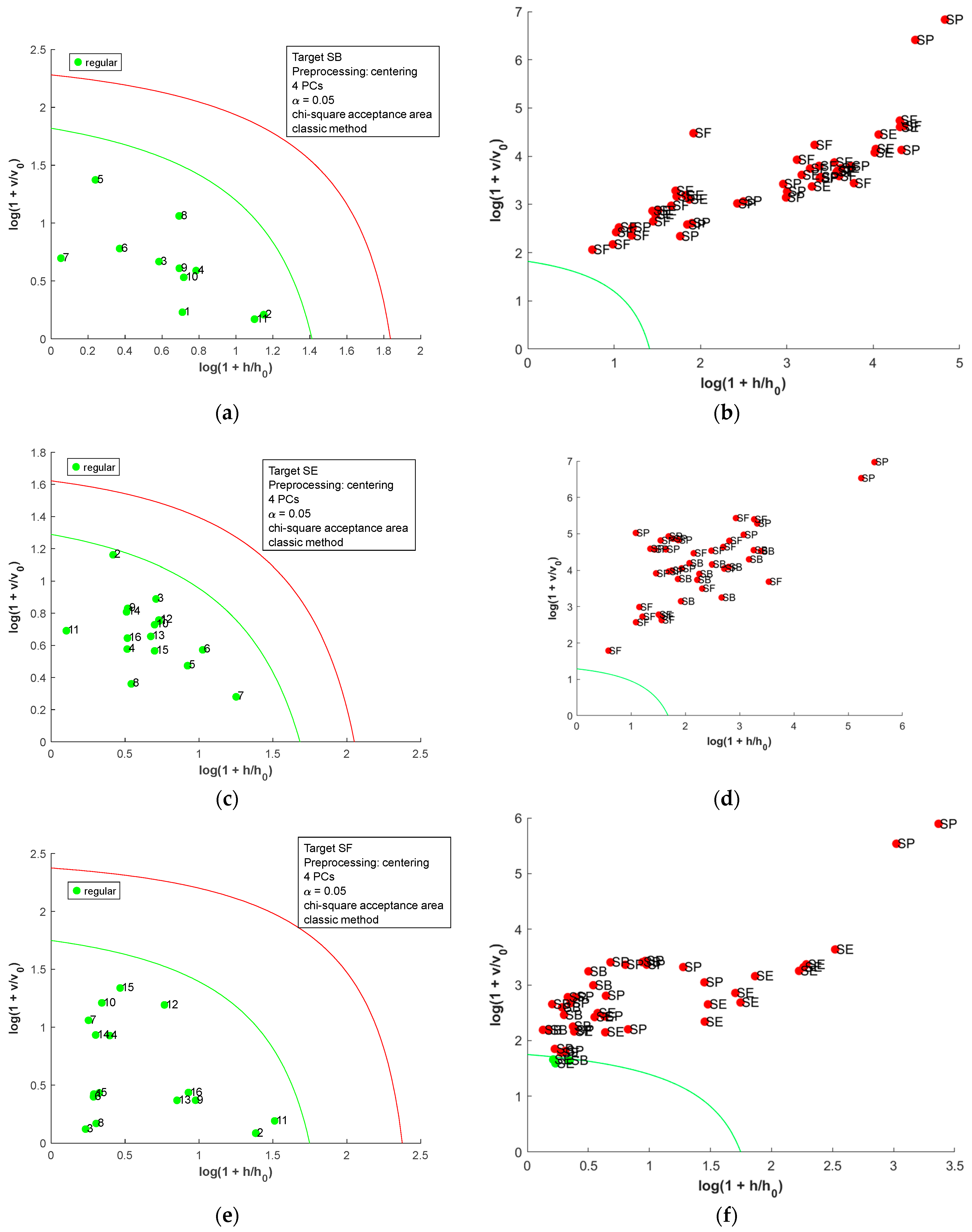
3.3. Near-Infrared Spectrometry

Figure 5a shows the effect of the sample preparation on the NIR spectra. Water content and particle–size distribution are two factors that directly influence the NIR spectrum [14]. Therefore, the effect of these two factors on the table salt classification is first discussed. The major differences occur in the 1300–1600 nm region, which contains the second overtone for water. It is possible to observe minor changes in the third overtone water region below 1000 nm. The effect of the salt origin on the spectra could be observed for raw, dried, and dried-milled salt, as presented in Figure 3b–d. The spectra profile is similar to other works [2,7].
A PCA (mean center matrix) of the sample’s spectra obtained for each country was performed to better understand the effect of sample treatment, and the results are summarized in Figure 6. For Brazilian salt (Figure 6a), the raw salt samples had positive scores in PC1 (except SB9 and SB11); the dried and dried-milled samples had negative scores in PC1 (except SB10 and SB8 for dried salt). Sample SB11 presented the lowest humidity (0.0246%); however, sample SB5 had the highest humidity (0.3771%) considering the Brazilian salt. Samples SB8 and SB10 were coarse salt; only after milling were these samples grouped with other Brazilian samples. The loading plot (Figure 6b) shows that regions 1300–1600 nm and below 1000 nm had a major influence on the separation observed in PC1. As mentioned before, these regions are related to the second and third water overtone, respectively. The distribution of the samples in the PC2 is maintained with the treatments applied to the salt samples. For example, SB9 always had negative scores in PC2, independent of the treatment used before NIR spectrum acquisition. On the other hand, SB10 or SP10 always had positive scores. For SF and SE, it is possible to see that samples were divided into two groups, which were the same regardless of the treatment used before NIR spectrum acquisition. Therefore, PC2 contains spectral information about the samples’ composition independent of granulometry or humidity.
For Spain, the circled and boxed groups are the same samples listed but for different treatments of the table salt (Figure 6c). The dried-milled salt samples form a separate group, and raw and dried salt samples form another group. Furthermore, SE samples were split into two groups. This separation is maintained regardless of the treatment applied to the samples. Comparing these two groups’ humidity and metal profiles (Table S3), it is possible to see a great difference between Mg and Mn. The separation between these two groups is mainly represented in PC1. The loading plots show that the 1350–1550 nm region has a higher weight for the distribution of the samples in PC1. Water can be associated with salts even after drying in an oven as saline hydrates. The water of hydration or crystallization refers to water found in the crystalline framework of a salt. The determination of salt by NIR is based on the behavior of the water component in the spectrum due to changes in hydrogen bonding, resulting in band shifts (aquaphotomic) [14]. When the salt-induced changes in the water spectrum can be isolated from other spectral variations, salt detection could be improved [23]. Thus, after eliminating humidity and granulometry standardization, the NIR spectra highlighted the absorption bands associated with water in saline hydrates. We acquired some spectra of magnesium chloride hexahydrate, manganese chloride tetrahydrate, sodium chloride, and mixtures to test this hypothesis (Figure S6). Before the spectra acquisition, the same procedure was used for salt preparation (drying and milling steps). These spectra confirmed that hydrate salts had bands in the 1300–1600 nm region. The spectra for SE12 (highest manganese content in SE samples) and SE13 (highest magnesium content in SE samples) were also plotted for comparison. Previous work also related these effects in near-infrared spectra [2].
Salt samples from France showed similar behavior to that observed for salt from Spain, separating into two groups regardless of the treatment applied. The circled and boxed groups are the same samples listed, but for different treatments of the table salt (Figure 6e). Comparing the other evaluated properties (Table S3) for these two groups, we observed variability in humidity, which is eliminated after drying. The metal profile showed major differences for potassium, calcium, magnesium, iron, and manganese. Figure S6c shows the NIR spectra for calcium chloride dihydrate and iron (III) chloride hexahydrate with absorption bands in the 1300–1600 nm region. Potassium chloride does not have water of hydration, so its spectrum is similar to sodium chloride. The spectra for SF2 (highest calcium content in SF samples) and SF13 (highest iron content in SF samples) were also plotted to compare with the hydrate salts.
Samples SP9, SP10, SP11, and SP16 were separated from the others for Portugal. These four samples were flower salt, which had more humidity, potassium, calcium, and magnesium (Table S3). Once again, NIR spectra separated salt according to minerals that form hydrates, resulting in a shift in the water band at ~1400 nm.
Considering that the sample’s treatment interferes with the analysis, a PCA for each salt treatment was performed to evaluate the effect of the countries in the salt spectra. For raw salt, it is possible to see in the loading plot (Figure 7b) that the samples’ distribution in PC1 is due to the 1350–1550 nm region, which contains the second overtone for water. The samples SP9, SF12, and SP16, highlighted in Figure 7a, had a higher positive score in PC1 and humidity (Table S1). There is a correlation between PC1 scores and sample humidity (r = 0.58, p-value = 1.43 × 10⁻⁶). Figure S7 confirms that higher correlations between the spectra’ first derivative and humidity occur in the 1350–1550 nm region. This correlation is not observed in PC2 (r = 0.19, p-value = 0.15). Otherwise, PC2 separates SB (positive scores) and SE (negative scores). The loading plot (Figure 7b) indicates the region below 1000 nm and between the range 1350 and 1500 nm, with a major contribution to this separation. Comparing the mean and median values for metal profile (Table 1) for SB and SE suggests that Fe, Cu, Mg, and Mn were the most important differences. However, PC2 scores (Figure 7a) did not present a higher correlation with the values for these metals (rMg = 0.09, pMg = 0.48, rFe = 0.32, pFe = 0.01, rMn = −0.22, pMn = 0.10, rCu = 0.38, pCu = 3.00 × 10⁻³). In the correlation plots between the raw salt spectra’ first derivative and metal content (Figure S8), Mn content correlated with the regions below 1000 nm and 1350–1500 nm, Mg and Fe contents correlated only with the last region, and Cu did not have important correlations. The DD-SIMCA was applied to the first derivative of NIR spectra for raw salt (Figure S9 and Table S5). Four PCs were necessary for better results, but nineteen samples were misclassified. Only SB was successfully classified; for SE, two samples of SP were misclassified; for SF, four samples of SE, two samples of SP, and one sample of SB were misclassified; for SP, ten samples of SE were misclassified.
For dried salt (Figure 7c), the distribution of the samples in PC1 and PC2 was related to the mineral content, as previously discussed. The granulometry differences may interfere with the distribution, but it is not easy to establish a relation between the grain size and PCA distribution. The DD-SIMCA using the dried salt spectra (Figure S10 and Table S5) performs the worst compared to other salt treatments and FAAS data, with twenty-three misclassifications. For SB, one sample of SE and one sample of SP were misclassified; for SE, one sample of SP and one sample of SB were misclassified; for SF, five samples of SE, one sample of SP, and one sample of SB were misclassified; for SP, six samples of SE and six samples of SB were misclassified.
For dried-milled salt (Figure 7e), it is possible to see (PC1) the same distribution in two groups for SE, SF, and SP, as previously in Figure 6. The SB samples remain grouped considering the PC1 and PC2 axes. Table 2 presents the correlations between the scores (PCA for dried-milled salt) and the metal content determined via FAAS.
The PC1 had significant correlations with Mg, Mn, and Cu; a negative correlation with Ca was observed. The samples with higher scores for PC1 (SP9, SF12, SF16, and others) also have higher values for Mg (Table S2). Otherwise, samples with lower scores for PC1 (for example, SF1 and SF15) have lower levels of Mg. The same behavior is presented for the other metals, with significant correlations with PC1, but it is less evident than the trend for Mg. The loadings for PC1 (Figure 6f) indicate that the 1300–1600 nm region had more weight for the observed distribution of the samples. As previously discussed, this region is related to the OH bond from the salts’ water of hydration, the aquaphotomic effect [14]. The correlation plot between the dried-milled salt spectra’ first derivative and metal contents (Figure S11) confirms that this region had higher correlations with Mg and Mn.
The PC2 mainly separates the SP9 and SP16 samples from the others. The correlations with PC2 scores indicate a relationship with Cu, Mg, and Mn. The loadings for PC2 have higher values for the region between 1350–1550 nm, near 1200 nm, and below 1000 nm. The first region correlates more with Mg and Mn, and the second and third regions correlate more with Cu (Figure S11).
The acceptance plots for the DD-SIMCA model using the first derivative of the dried-milled salt NIR spectra are presented in Figure 8. Only three misclassifications, false positives, were observed; two SE (SE7 and SE8, labeled as sea salt) and one SB (SB10, labeled refined salt) samples were classified as SF. Therefore, DD-SIMCA models reached 100% sensitivity and were 100% specific for SB, SE, and SP. For SF, the DD-SIMCA model was 100% sensitive and 93.0% specific. A comparison between all DD-SIMCA models was provided in Table S5 in the Supplementary Material. The classification performance for NIR spectra of the dried-milled salt was superior to that for FAAS data. Furthermore, the NIR has less sample preparation, cost, and time consumption than FAAS.
It is important to highlight that possible correlations between the elements quantified using FAAS and the NIR spectra were analyzed. However, other elements different from those quantified may also interfere with the water of hydration and, consequently, with the NIR spectrum of the sample. Thus, better classification performance was obtained with the NIR spectra because other unidentified elements may be contributing to differentiating the origin of the different table salts analyzed.

4. Conclusions

The FAAS spectroscopy showed differences between the mineral content of the salts from Brazil, Spain, France, and Portugal, with major differences for Ca, Mg, Fe, Mn, and Cu. A large variation in the amount of minerals was also observed for samples from the same country. The DD-SIMCA model, using the FAAS data, separated the salt according to the country of origin with few misclassifications.
The granulometry and humidity were important parameters that interfered with the NIR spectra. The NIR spectra presented absorption bands related to the humidity in the salt and with water of hydration from some salts. After drying, the NIR spectra for salt samples showed a higher correlation with Mg, Mn, and Cu contents. The DD-SIMCA model using the spectra for dried-milled samples had a similar performance (three misclassifications) compared to the FAAS data.
Both FAAS and NIR spectroscopy identified the origin of the salt samples, but NIR is a simpler and faster analysis that produces results equivalent to FAAS. Our results demonstrate a great variability in the composition of table salt from different countries. These data reinforce the importance of using accurate analytical methods, such as FAAS and alternative instruments, and portable NIR, to authenticate the origin or detect possible fraud in table salt. In future work, it will be important to analyze more samples, including more countries and products with fraud, and verify the possibility of using other machine learning algorithms to interpret and model the data obtained.

Supplementary Materials

The following supporting information can be downloaded at: https://www.mdpi.com/article/10.3390/chemosensors13070231/s1, Table S1: Humidity for salt samples (SB—Brazilian salt; SE—Spain salt; SF—France salt; and SP—Portugal salt); Table S2: Metals quantified (dry basis) using flame atomic absorption spectrometry (FAAS); Table S3: Comparison between the mean humidity and content of metals between samples with positive scores in PC2 and the negative scores in PC2; Table S4: Calibration curves for quantification of mineral composition; Table S5: Comparison between all DD-SIMCA models; Figure S1: Raw salt from Brazil; Figure S2: Raw salt from Spain; Figure S3: Raw salt from France; Figure S4: Raw salt from Portugal; Figure S5: PCA of the autoscaled matrix of the mineral content: (a) Pareto plot with the variance and accumulated variance; (b) Scree plot with eigenvalues; (c) Bar plot with variance extract for each variable in each principal component. Figure S6: Comparison between NIR spectra of some salt samples, magnesium chloride hexahydrate, manganese chloride tetrahydrate, iron (III) chloride hexahydrate, calcium chloride dihydrate, sodium chloride, potassium chloride, and mixtures. Figure S7: Correlation between the raw salt spectra’ first derivative and humidity represented with colors in the mean first derivative plot. Figure S8: Correlation between the raw salt spectra’ first derivative and metal content represented with colors in the mean first derivative plot: (a) Mg, (b) Fe, (c) Mn, and (d) Cu. Figure S9: Acceptance plots for DD-SIMCA using the first derivative of NIR spectra from raw salt: (a) target class SB; (b) test class SE, SF, and SP; (c) target class SE; (d) test class SB, SF, and SP; (e) target class SF; (f) test class SB, SE, and SP; (g) target class SP; (h) test class SB, SE, and SF. Figure S10: Acceptance plots for DD-SIMCA using the first derivative of NIR spectra from dried salt: (a) target class SB; (b) test class SE, SF, and SP; (c) target class SE; (d) test class SB, SF, and SP; (e) target class SF; (f) test class SB, SE, and SP; (g) target class SP; (h) test class SB, SE, and SF. Figure S11: Correlation between the dried-milled salt spectra’ first derivative and metal content represented with colors in the mean first derivative plot: (a) K, (b) Na, (c) Ca, (d) Mg, (e) Fe, (f) Mn, (g) Zn, and (h) Cu.

Author Contributions

All authors contributed to the study’s conception and design. Material preparation, data collection, and analysis were performed by E.B., L.R.Z.L., L.D.d.S., I.T., D.C., F.L.M., L.G.D., L.E., and E.B. wrote the first draft of the manuscript, and all authors commented on previous versions. All authors have read and agreed to the published version of the manuscript.

Funding

This work was supported by Conselho Nacional de Desenvolvimento Científico e Tecnológico (CNPq)—grant numbers 312595/2021-2, 310446/2020-1, INCT-FNA 464898/2014-5; Foundation for Science and Technology (FCT, Portugal) for financial support through national funds FCT/MCTES (PIDDAC) to CIMO (UIDB/00690/2020 and UIDP/00690/2020) and SusTEC (LA/P/0007/2020).

Data Availability Statement

The datasets generated and analyzed during the current study are available from the corresponding authors upon reasonable request.

Acknowledgments

The authors are thankful for the support in the measurements of UTFPR, Central Analítica Multiusuário at UTFPR Campus Campo Mourão (CAMulti-CM).

Conflicts of Interest

The authors declare no conflicts of interest.

References

  1. Kuhn, T.; Chytry, P.; Souza, G.M.S.; Bauer, D.V.; Amaral, L.; Dias, J.F. Signature of the Himalayan Salt. Nucl. Instrum. Methods. Phys. Res. B 2020, 477, 150–153. [Google Scholar] [CrossRef]
  2. Galvis-Sánchez, A.C.; Lopes, J.A.; Delgadillo, I.; Rangel, A.O.S.S. Fourier Transform Near-Infrared Spectroscopy Application for Sea Salt Quality Evaluation. J. Agric. Food Chem 2011, 59, 11109–11116. [Google Scholar] [CrossRef] [PubMed]
  3. Da-Col, J.A.; Bueno, M.I.M.S.; Melquiades, F.L. Fast and Direct Na and K Determination in Table, Marine, and Low-Sodium Salts by X-Ray Fluorescence and Chemometrics. J. Agric. Food Chem. 2015, 63, 2406–2412. [Google Scholar] [CrossRef] [PubMed]
  4. Galiga, H.F.; Sevilla, F.B. Smartphone-Based Optical Transduction for the Rapid Microscale Assessment of Iodate in Table Salt. Talanta 2021, 232, 122450. [Google Scholar] [CrossRef] [PubMed]
  5. Hassoun, A.; Siddiqui, S.A.; Smaoui, S.; Ucak, İ.; Arshad, R.N.; Bhat, Z.F.; Bhat, H.F.; Carpena, M.; Prieto, M.A.; Aït-Kaddour, A.; et al. Emerging Technological Advances in Improving the Safety of Muscle Foods: Framing in the Context of the Food Revolution 4.0. Food Rev. Int. 2024, 40, 37–78. [Google Scholar] [CrossRef]
  6. Soylak, M.; Murat, I. Determination of Copper, Cobalt, Lead, and Iron in Table Salt by FAAS After Separation Using Violuric Acid and Multiwalled Carbon Nanotubes. Food Anal. Methods 2012, 5, 1003–1009. [Google Scholar] [CrossRef]
  7. Gowen, A.A.; Marini, F.; Tsuchisaka, Y.; De Luca, S.; Bevilacqua, M.; O’Donnell, C.; Downey, G.; Tsenkova, R. On the Feasibility of near Infrared Spectroscopy to Detect Contaminants in Water Using Single Salt Solutions as Model Systems. Talanta 2015, 131, 609–618. [Google Scholar] [CrossRef] [PubMed]
  8. Fodor, M.; Matkovits, A.; Benes, E.L.; Jókai, Z. The Role of Near-Infrared Spectroscopy in Food Quality Assurance: A Review of the Past Two Decades. Foods 2024, 13, 3501. [Google Scholar] [CrossRef]
  9. Spoladore, S.F.; Brígida dos Santos Scholz, M.; Bona, E. Genotypic Classification of Wheat Using Near-Infrared Spectroscopy and PLS-DA. Appl. Food Res. 2021, 1, 100019. [Google Scholar] [CrossRef]
  10. Francielli Vieira, T.; Makimori, G.Y.; Scholz, M.B.; Zielinski, A.; Bona, E. Chemometric Approach Using ComDim and PLS-DA for Discrimination and Classification of Commercial Yerba Mate (Ilex paraguariensis St. Hil.). Food Anal. Methods 2020, 13, 97–107. [Google Scholar] [CrossRef]
  11. de Andrade, J.C.; Galvan, D.; Effting, L.; Lelis, C.; Melquiades, F.L.; Bona, E.; Conte-Junior, C.A. An Easy-to-Use and Cheap Analytical Approach Based on NIR and Chemometrics for Tomato and Sweet Pepper Authentication by Non-Volatile Profile. Food Anal. Methods 2023, 16, 567–580. [Google Scholar] [CrossRef]
  12. Galvan, D.; Lelis, C.A.; Effting, L.; Melquiades, F.L.; Bona, E.; Conte-Junior, C.A. Low-Cost Spectroscopic Devices with Multivariate Analysis Applied to Milk Authenticity. Microchem. J. 2022, 181, 107746. [Google Scholar] [CrossRef]
  13. Frost, V.J.; Molt, K. Analysis of Aqueous Solutions by Near-Infrared Spectrometry (NIRS) III. Binary Mixtures of Inorganic Salts in Water. J. Mol. Struct. 1997, 410–411, 573–579. [Google Scholar] [CrossRef]
  14. Pasquini, C. Near Infrared Spectroscopy: A Mature Analytical Technique with New Perspectives—A Review. Anal. Chim. Acta 2018, 1026, 8–36. [Google Scholar] [CrossRef] [PubMed]
  15. Março, P.; Bona, E.; Valderrama, P. Chapter 4—Chemometrics Applied to Food Control. In Food Control and Biosecurity; Academic Press: Cambridge, MA, USA, 2018. [Google Scholar]
  16. Galvan, D.; Aquino, A.; Effting, L.; Mantovani, A.C.G.; Bona, E.; Conte-Junior, C.A. E-Sensing and Nanoscale-Sensing Devices Associated with Data Processing Algorithms Applied to Food Quality Control: A Systematic Review. Crit. Rev. Food Sci. Nutr. 2022, 62, 6605–6645. [Google Scholar] [CrossRef] [PubMed]
  17. Granato, D.; Putnik, P.; Kovačević, D.B.; Santos, J.S.; Calado, V.; Rocha, R.S.; Da Cruz, A.G.; Jarvis, B.; Rodionova, O.Y.; Pomerantsev, A. Trends in Chemometrics: Food Authentication, Microbiology, and Effects of Processing. Compr. Rev. Food Sci. Food Saf. 2018, 17, 663–677. [Google Scholar] [CrossRef] [PubMed]
  18. Rodionova, O.Y.; Titova, A.V.; Pomerantsev, A.L. Discriminant Analysis Is an Inappropriate Method of Authentication. TrAC Trends Anal. Chem. 2016, 78, 17–22. [Google Scholar] [CrossRef]
  19. Zontov, Y.V.; Rodionova, O.Y.; Kucheryavskiy, S.V.; Pomerantsev, A.L. DD-SIMCA—A MATLAB GUI Tool for Data Driven SIMCA Approach. Chemom. Intell. Lab. Syst. 2017, 167, 23–28. [Google Scholar] [CrossRef]
  20. Pomerantsev, A.L.; Rodionova, O.Y. Concept and Role of Extreme Objects in PCA/SIMCA. J. Chemom 2014, 28, 429–438. [Google Scholar] [CrossRef]
  21. Instituto Adolfo Lutz. Métodos Físico-Químicos Para Análise de Alimentos; Zenebon, O., Pascuet, N.S., Tiglea, P., Eds.; Instituto Adolfo Lutz: Sao Paulo, Brazil, 2008.
  22. Kucheryavskiy, S.; Rodionova, O.; Pomerantsev, A. A Comprehensive Tutorial on Data-Driven SIMCA: Theory and Implementation in Web. J. Chemom. 2024, 38, e3556. [Google Scholar] [CrossRef]
  23. Burns, D.A.; Ciurczak, E.W. Handbook of Near-Infrared Analysis, 3rd ed.; CRC Press: Boca Raton, FL, USA, 2007; ISBN 9780429123016. [Google Scholar]
Figure 1. Box plot for humidity variation according to each country.
Chemosensors 13 00231 g001
Figure 2. Radar plot for each mean metal content (mean values) based on the country of the salt. For sodium concentration, the unit is mg g−1. For the other metals, the concentration unit is µg g−1.
Chemosensors 13 00231 g002
Figure 3. Principal component analysis of the autoscaled mineral content matrix: score plot for the first four PCs (a), loadings for PC1 (b), PC2 (c), PC3 (d), and PC4 (e).
Chemosensors 13 00231 g003aChemosensors 13 00231 g003b
Figure 4. Acceptance plots for DD-SIMCA using the metal content table: (a) target class SB; (b) test class SE, SF, and SP; (c) target class SE; (d) test class SB, SF, and SP; (e) target class SF; (f) test class SB, SE, and SP; (g) target class SP; and (h) test class SB, SE, and SF. The green line is the acceptance border, and the red line is the outlier border.
Chemosensors 13 00231 g004aChemosensors 13 00231 g004b
Figure 5. The first derivative of the NIR spectra: effect of the salt preparation in the spectra (a); effect of the country of origin in the spectra of raw salt (b), dried salt (c), and dried-milled salt (d).
Chemosensors 13 00231 g005
Figure 6. PCA for the mean-centered first derivative of the spectra for the raw, dried, and dried-milled samples of each country: (a) score plot and (b) loading plot for SB; (c) score plot and (d) loading plot for SE; (e) score plot and (f) loading plot for SF; and (g) score plot and (h) loading plot for SP.
Chemosensors 13 00231 g006aChemosensors 13 00231 g006b
Figure 7. PCA of the mean-centered first derivative of the spectra of the four countries for each salt treatment: (a) score plot and (b) loading plot for raw salt; (c) score plot and (d) loading plot for dried salt; and (e) score plot and (f) loading plot for dried-milled salt.
Chemosensors 13 00231 g007
Figure 8. Acceptance plots for DD-SIMCA using the first derivative of NIR spectra from dried-milled salt of each country: (a) target class SB; (b) test class SE, SF, and SP; (c) target class SE; (d) test class SB, SF, and SP; (e) target class SF; (f) test class SB, SE, and SP; (g) target class SP; (h) test class SB, SE, and SF. The green line is the acceptance border, and the red line is the outlier border.
Chemosensors 13 00231 g008aChemosensors 13 00231 g008b
Table 1. Descriptive statistics for metals quantified using FAAS.
CountryMinimumMaximumMedian *Mean **Standard Deviation
K (µg g−1)
SB1694.22 × 103251 a1.21 × 103 a1.66 × 103
SE1261.23 × 103356 a379 a242
SF36.93.42 × 105770 a2.20 × 104 a8.54 × 104
SP65.04.03 × 103296 a711 a1.04 × 103
Na (mg g−1)
SB341648421 ab451 a94.7
SE382557418 b441 a51.3
SF134601400 a398 a89.9
SP177606415 ab404 a121
Ca (µg g−1)
SB3471.05 × 103540 b593 b203
SE97.21.08 × 103610 b569 b274
SF1131.81 × 103355 b692 b596
SP0.6221.23 × 10377.7 a154 a299
Mg (µg g−1)
SB77.9635132 a236 a174
SE35.21.45 × 103867 b719 a530
SF21.87.28 × 1031.61 × 103 ab2.20 × 103 b2.37 × 103
SP4.176.06 × 103580 b1.16 × 103 ab1.56 × 103
Fe (µg g−1)
SB0.28653.31.80 b7.09 ab15.4
SE0.0272.340.127 a0.579 a0.854
SF0.01871050.869 abc19.5 b31.6
SP1.708.795.09 c5.17 ab2.01
Mn (µg g−1)
SB0.1111.110.545 a0.616 a0.327
SE0.01262.691.86 b1.42 a1.00
SF0.01116.551.16 ab1.89 a1.95
SP1.527.083.81 c4.08 b1.58
Zn (µg g−1)
SB0.1030.2700.192 a0.193 a0.0480
SE0.008930.6010.229 a0.267 a0.152
SF0.2081.200.562 b0.602 b0.227
SP0.07900.8530.506 b0.471 b0.242
Cu (µg g−1)
SB0.3571.930.445 bc0.737 bc0.564
SE0.06630.4250.196 a0.186 a0.0941
SF0.1250.7750.444 b0.445 ab0.136
SP0.2661.540.942 c0.948 c0.383
* Median values with different letters are statistically different (p-value < 0.05) in Wilcoxon’s rank sum test. ** Mean values with different letters are statistically different (p-value < 0.05) in Tukey’s test.
Table 2. Correlations between PC1 and PC2 scores (dried-milled salt) and the metal content of the samples.
MetalPC1PC2
K−0.12300.0572
Na−0.1350−0.0019
Ca−0.3409 *−0.0396
Mg0.7503 *0.2969 *
Fe0.22140.0444
Mn0.6573 *0.2701 *
Zn0.3896 *0.2155
Cu0.05820.4787 *
* Statistically significant correlations (p < 0.05).
Disclaimer/Publisher’s Note: The statements, opinions and data contained in all publications are solely those of the individual author(s) and contributor(s) and not of MDPI and/or the editor(s). MDPI and/or the editor(s) disclaim responsibility for any injury to people or property resulting from any ideas, methods, instructions or products referred to in the content.

