Abstract
Visible near-infrared (Vis-NIR) spectroscopy is widely used for rapid soil element detection, but calibration models are often limited by instrument-specific constraints, including varying laboratory conditions and sensor configurations. To address this, we propose a novel calibration transfer method that eliminates the conventional requirement of designating ‘master’ and ‘slave’ devices. Instead, spectral data from two spectrometers are fused to create a master spectrum, while independent spectral data serve as slave spectra. We developed an ensemble stacking model, incorporating partial least squares regression (PLSR), support vector regression (SVR), and ridge regression (Ridge) in the first layer, with BoostForest (BF) as the second layer, trained on the fused master spectrum. This model was further integrated with three calibration transfer methods: direct standardization (DS), piecewise direct standardization (PDS), and spectral space transfer (SST), to enable seamless application across slave spectra. Applied to soil total nitrogen (TN) detection, the method achieved an R2P of 0.842, RMSEP of 0.017, and RPD of 2.544 on the first slave spectrometer, and an R2P of 0.830, RMSEP of 0.018, and RPD of 2.452 on the second. These results demonstrate the method’s ability to simplify calibration processes while enhancing cross-instrument prediction accuracy, supporting robust and generalizable cross-instrument applications.
1. Introduction
Soil is a critical, complex ecosystem intersecting the Earth’s atmosphere, lithosphere, hydrosphere, and biosphere. It forms the essential base for food production and is central to sustainable development [1]. Soil fertility, crucial for crop growth, yield, and quality, is influenced by factors including organic matter, organic carbon, pH, and levels of phosphorus, potassium, and especially total nitrogen (TN), a key indicator of fertility [2]. However, the lack of real-time data on soil TN often leads farmers to over-apply fertilizers to ensure crop productivity. This practice not only burdens the environment and escalates economic costs but also has adverse effects on ecosystems, particularly when fertilizers run off into water systems, damaging ecosystem services [3]. Accurate, timely knowledge of soil TN is vital for precise fertilizer application.
Traditional soil testing methods are laboratory-based and, while accurate, are time-consuming and resource-intensive. These methods fail to provide real-time, continuous soil data, which is crucial for informed decision-making in modern agriculture [4]. Thus, there is a pressing need for new methodologies that offer quick, economical, and reasonably accurate soil property predictions. Visible near-infrared (Vis-NIR) spectroscopy has recently emerged as an effective tool for soil analysis [5]. The physical and chemical properties of soil interact with energy in the Vis-NIR range, producing characteristic absorption features in the spectrum. These absorption features correspond to specific soil minerals and organic components. Therefore, by analyzing spectral data, it is possible to conduct quantitative analysis of certain soil characteristics, including organic carbon, TN, and others [6]. For example, in the case of TN, the C=O, C–H, O–H, and N–H bonds in the Vis-NIR spectral range are highly correlated with TN in soils [7]. However, the Vis-NIR spectrum cannot be visually analyzed and interpreted with ease. Coupled with advanced machine learning techniques, Vis-NIR has become a viable alternative to traditional lab analyses for assessing soil properties [8]. This technology is employed to measure soil organic carbon [9], pH [10], total phosphorus [11], total potassium [12], and TN [13], among other properties. Vis-NIR spectroscopy is fast and non-destructive and reduces the need for sample pre-treatment and chemical processes, thereby diminishing environmental impacts. It can assess multiple soil properties in a single scan, showcasing its versatility and adaptability in both laboratory and field settings [14].
When employing Vis-NIR spectroscopy for soil analysis, calibration models are typically tailored to specific spectrometers, designed by various researchers. However, discrepancies in wavelength and spectral response among instruments can hinder the transferability of these models across different devices [15]. This limitation restricts the universal applicability of a model, as adapting a model for a new spectrometer can be both costly and time-consuming, slowing the adoption of Vis-NIR spectroscopy. To overcome these challenges, chemometric techniques such as calibration transfer methods are utilized. These methods facilitate the alignment of instrument differences, thereby enabling the cross-instrument application of models [16]. They designate the original spectrometer as the ‘master’ and the new spectrometer as the ‘slave’. Techniques such as direct standardization (DS) [17], piecewise direct standardization (PDS) [17], and spectral space transfer (SST) [18] are employed to harmonize the slave’s spectra with that of the master, allowing the direct use of pre-established spectral models on the slave device [19].
Additionally, the integration of spectral data from multiple sensors through a multi-sensor spectral data fusion approach enhances the robustness and accuracy of the models. This technique aggregates complementary information from various data sources, enriching the model’s input and improving prediction capabilities when combined with advanced machine learning algorithms [20,21]. However, the application of spectral data fusion in conjunction with calibration transfer methods for soil analysis in the Vis-NIR spectrum has not been widely documented, and the effects of such integrations on model transferability remain to be explored.
Moreover, the ensemble stacking model, an advanced machine learning strategy, has been shown to enhance predictive performance by leveraging the unique strengths of various models. This method amalgamates different model outputs to produce more precise and reliable results [22]. Recent studies suggest that combining Vis-NIR spectroscopy with an ensemble stacking model yields more accurate soil element predictions than traditional calibration models alone [23,24]. Currently, most calibration transfer methods in soil testing primarily focus on transferring classical partial least squares regression (PLSR) models [25,26]. Further research is required to determine whether ensemble stacking can serve as an effective transfer model to improve prediction accuracy on new instruments.
Therefore, the objectives of this study are as follows: (1) to collect spectral data from a consistent batch of standard soil samples using two different Vis-NIR spectrometers to establish calibration models for soil TN separately, (2) to evaluate the effectiveness of different calibration transfer methods in transferring the TN calibration model from the original spectrometer (master) to a new spectrometer (slave), (3) to investigate the potential of enhancing model transfer by combining spectral data fusion with calibration transfer methods, and (4) to develop an ensemble stacking model to serve as a transfer model, leveraging multiple calibration models to improve prediction accuracy.
2. Materials and Methods
2.1. Soil Samples and Total Nitrogen Measurement
A total of 168 soil samples were collected for the study, comprising 118 samples from Zhejiang Province and 50 from Jiangxi Province in China. Soil samples were placed in sealed bags and brought back to the laboratory. The collected soil samples were air-dried, ground, and sieved through a 60-mesh screen in the laboratory. Each sample was then divided into four portions in Petri dishes: three portions were used to collect Vis-NIR spectra for calculating the average spectrum, while the remaining portion was analyzed by flow injection to determine soil TN content [27]. Soil TN content was measured by a professional testing agency to ensure the accuracy and reliability of the experimental data. The agency information is detailed in the Supplementary Materials.
2.2. Vis-NIR Spectra Collection and Data Pre-Processing
This section details the collection and pre-processing of Vis-NIR spectral data for soil sample analysis. Spectral data from 168 soil samples were obtained using two different spectrometers: the Oceanhood OFS spectrometer (Oceanhood Opto-electronics Technology Co., Ltd., Shanghai, China) and the Optosky ATP9110 spectrometer (Optosky Technology Co., Ltd., Xiamen, China). The Oceanhood spectrometer captures wavelengths from 342 nm to 2504 nm. The instrument’s built-in interpolation algorithm outputs spectral wavelengths spaced at 1 nm intervals, resulting in 2163 variables. For the spectral range of 342 nm to 900 nm, the spectral resolution is 2.5 nm, and the signal-to-noise ratio (SNR) is 500:1. For the range of 900 nm to 2504 nm, the spectral resolution is 8 nm, and the SNR is 2000:1. Conversely, the Optosky spectrometer records wavelengths ranging from 282.36 nm to 2529.431 nm, encompassing 2325 variables. For the spectral range of 282.36 nm to 1000 nm, the spectral resolution is 2.429 nm, and the SNR is 800:1. For the range of 1000 nm to 2529.431 nm, the spectral resolution is 7.687 nm, and the SNR is 16,000:1. To harmonize the data from both devices for model transfer, Cubic Spline Interpolation was applied to standardize spectral intervals at 1 nm across the entire wavelength range. Both instruments were set with an integration time of 8 milliseconds and a sampling interval of 1000 milliseconds. They performed 50 smoothing and averaging scans. Calibration with black and white reference plates was conducted after every 15 sample collections. For each soil sample, reflectance values were averaged from three parallel measurements to determine the final spectrum. In terms of data pre-processing, noise at the beginning and end of the spectra was removed, narrowing the analysis range to 400 nm to 2450 nm, which standardized the resolution and reduced the variable count to 2051. The spectra were smoothed using Savitzky–Golay (SG) smoothing, employing a second-order polynomial fit and an 11-point window [28]. We performed the aforementioned preprocessing on the spectra to enhance the SNR of the spectral data. This step was performed using Unscrambler X 10.4 software (CAMO Software AS, Oslo, Norway). For clarity in further discussions, the Oceanhood and Optosky spectrometers are henceforth referred to as Spectrometer No. 1 and Spectrometer No. 2, respectively.
2.3. Spectral Data Fusion
The methodology for spectral data fusion used in our study aims to create a comprehensive dataset by integrating spectral information from multiple sources [29]. Our focus is on data-layer fusion, a method that involves the statistical analysis of raw observations from each sensor. This approach is designed to maintain a high degree of the original data’s integrity by emphasizing the correlation among raw datasets. In our experiment, we applied data-layer fusion to combine data from two distinct Vis-NIR spectrometers. The spectral data from these instruments were fused into what we term the ‘master spectrum’, which is used for model transfer while maintaining them as ‘slave spectra’ to minimize spectral variability between the datasets. This fusion process involves assigning specific weights to the spectral data from each spectrometer before summing them to form a new master spectrum. This technique allows the fused master spectrum to retain substantial information from both original datasets, thereby significantly reducing the spectral differences between the master and the slave spectra.
2.4. Calibration Models
In this study, we used the Kennard–Stone method [30] to segment the data from Spectrometer No. 2 into calibration and prediction sets, 70% for calibration and 30% for prediction. The same division strategy was applied to the data from Spectrometer No. 1 to maintain consistency across both instruments. The distribution of TN content, corresponding to the calibration and prediction sets, is detailed in Table 1. The close proximity of the mean and standard deviation values between the calibration and prediction sets indicates that these sets are well represented.

Table 1.
Statistics of measured soil total nitrogen content for the calibration and prediction sets.
We constructed a TN calibration model on the master spectrometer using an ensemble stacking approach and transferred the model to the slave spectrometer. This involved integrating three classical algorithms: PLSR, support vector regression (SVR), and ridge regression (Ridge), each serving as a foundational layer within the ensemble model.
2.4.1. PLSR
This method is effective in handling the challenges of multidimensionality among predictor variables, operating under the assumption of a linear relationship between predictors and responses. More details of this model can be found in [31]. The PLSR model is implemented using the PLSRegression function from the Scikit-learn library in Python 3.10.9, and the development environment is Jupyter Notebook (Project Jupyter, Berkeley, CA, USA).
2.4.2. SVR
Originating from supervised classification tasks, SVR is now extensively used in regression problems. It constructs an optimal hyperplane in a high-dimensional space to distinguish between closely related classifications. More details of this model can be found in [32]. The SVR model is implemented using the SVR function from the Scikit-learn library in Python 3.10.9, and the development environment is Jupyter Notebook.
2.4.3. Ridge
This method extends the least squares estimation by incorporating a penalty on the size of coefficients to address collinearity among predictor variables, thereby enhancing the reliability of regression coefficients. More details of this model can be found in [33]. The Ridge model is implemented using the Ridge function from the Scikit-learn library in Python 3.10.9, and the development environment is Jupyter Notebook.
2.4.4. Ensemble Stacking Model
In our research, we implemented an ensemble stacking model to enhance the accuracy of model transfers in soil detection using Vis-NIR spectroscopy. This model combines multiple machine learning algorithms, structured in two layers: the base models and the meta-model.
Base Models (First Layer): The first layer comprises three base models: PLSR, SVR, and Ridge. These models serve as the initial analytical step, providing preliminary predictions.
Meta-Model (Second Layer): The second layer uses a meta-model called BoostForest (BF), which is an innovative combination of Boosting and Bagging principles. BoostForest incorporates a novel decision tree approach, BoostTree, where each node in the tree houses a regression model. This model classifies inputs to a specific leaf and then aggregates the outputs from all nodes along the input’s path to generate a final prediction. BoostTree benefits from a unique parameter tuning strategy via random parameter pool sampling, simplifying hyperparameter adjustments compared to traditional methods. Using bootstrapping, BoostForest trains multiple BoostTrees on various copies of the original calibration set, enhancing model robustness and accuracy [34].
The establishment process of an ensemble stacking model is as follows. The calibration set is subdivided into five parts for 5-fold cross-validation, ensuring that each subset serves as a calibration set four times and a validation set once. For each fold, PLSR, SVR, and Ridge models are trained on four subsets and validated on the fifth, producing predictions for both the validation subset and the full prediction set. The predictions from the validation subsets are compiled into a new training dataset, while predictions from the prediction set are averaged to form a new predicted dataset. BoostForest, consisting of ten BoostTree models, is trained on this newly formed training dataset and subsequently used to predict the outcomes based on the new prediction set. This methodology minimizes overfitting and leverages the strengths of diverse predictive algorithms. Both the ensemble stacking model and the BoostForest model were implemented using Python 3.10.9, with the development environment being Jupyter Notebook, utilizing the StackingCVRegressor function from the mlxtend library and the BoostForestRegressor function from the BoostForest library, respectively. The structural and operational details of this model are illustrated in Figure 1, which demonstrates the comprehensive procedure from data division to final prediction aggregation, ensuring clarity in our model’s application and efficacy.
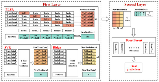
Figure 1.
The structure of our ensemble stacking model.
2.4.5. Hyperparameter Tuning
In our research, the process of hyperparameter tuning was meticulously structured to optimize the performance of the models employed in our ensemble stacking framework.
Latent Variables (LVs) in PLSR: We employed 5-fold cross-validation to ascertain the optimal number of LVs for the PLSR model. This approach helps in determining the most effective number of LVs to maximize model accuracy.
Parameter Optimization in SVR and Ridge Models: For the SVR and Ridge models, parameters were fine-tuned using Bayesian optimization, also within a 5-fold cross-validation framework [35]. Bayesian optimization is a strategy that seeks the best parameter settings to minimize the cross-validated mean square error. This method efficiently narrows down the most effective parameters by constructing a probabilistic model that maps parameter choices to their likely predictive performance.
BoostForest Meta-Model Tuning: Similarly, the meta-model BoostForest underwent parameter tuning through Bayesian optimization. This optimization was conducted on a new calibration set generated by the initial stacking and cross-validation of base models. This step ensures that the parameters selected contribute to an ensemble model that robustly predicts new data while minimizing error.
Iterative Optimization and Reproducibility: The number of iterations for the Bayesian optimizations was set to 50. After these iterations, the parameter set that yielded the lowest negative mean square error was chosen to construct each model. Additionally, to ensure consistency and reproducibility of the tuning process, a random seed was fixed at 42. Through this systematic approach to hyperparameter tuning, each model within our ensemble stacking architecture was optimized for maximum predictive performance, laying a robust foundation for accurate soil analysis using advanced spectroscopic techniques. The parameters of each model and the search range are as follows: SVR uses a regularization parameter C ranging from 10−2 to 102 and an error tolerance epsilon from 10−2 to 1 and employs the radial basis function (RBF) kernel. Ridge’s regularization strength alpha varies from 10−15 to 102. BoostForest sets max_leafs between 5 and 15, min_sample_leaf_list from 5 to 50 in increments of 5, and L1 regularization reg_alpha_list from 10−5 to 1. These parameters help control model complexity and regularization to enhance model performance.
2.5. Calibration Transfer Methods
To establish a link between spectra acquired by two different Vis-NIR spectrometers, we chose three classical calibration transfer methods: DS, PDS, and SST, which establish a transformation matrix F between the spectra through the corresponding spectra of the standard samples acquired on the master and slave. This matrix represents the difference between the spectra acquired by the master and slave and can be expressed in the form of multiplication of the slave spectra Xs with the transformation matrix F to obtain the master spectra Xm, which in turn enables the predicted result calibration.
Xm = XsF
DS is a method for directly solving the transformation matrix using the standard spectra of the master and the slave spectrometers using the principle of least squares. More details of this method are given in [17]. The DS method was implemented using PLS_Toolbox version 9.3 (Eigenvector Research Inc., Wenatchee, WA, USA) based on MATLAB R2022a (The Mathworks Inc., Natick, MA, USA).
To minimize errors due to regional variations in spectral differences, PDS utilizes localized spectra within a window for model transfer. Since spectral variations are usually limited to small regions, the window size is important for the performance of the PDS. If the value of the window size is too large, it retains too much redundant information. Conversely, the spectra in the window do not retain enough structural information [36]. More details of this method are given in [17]. We set the window size to an odd number in the range of 1 to 31 and select the most appropriate window size through the prediction results transferred by the PLSR model. The PDS method was implemented using PLS_Toolbox version 9.3 based on MATLAB R2022a.
SST is an algorithm for model transfer using standard spectra to construct a difference spectral projection space, the PCA loadings are utilized to develop the calibration transfer method. More details of this method are given in [18]. The SST method was implemented by writing functions using MATLAB 2022a.
2.6. Calibration Transfer Flowchart
A comparison between the standard calibration transfer method and our novel approach is depicted in Figure 2. Both methods are designed to transfer spectral models for soil analysis using Vis-NIR spectroscopy. Below is a streamlined description of the process, ensuring clarity and coherence in the presentation of methods.
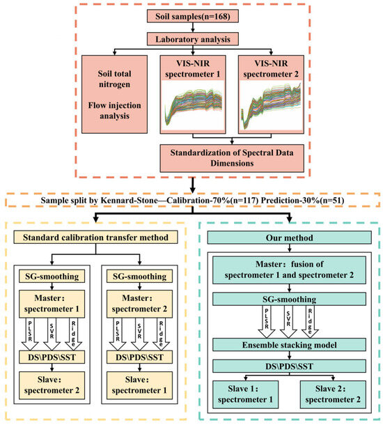
Figure 2.
Comparison flowchart depicting the standard calibration transfer method versus our novel approach. In the two spectra, the same color of the spectral lines means that they are from the same sample. The higher-resolution spectra are provided in the Supplementary Materials.
Initially, the TN content in soil samples was determined using flow injection analysis. Spectra from these samples were then acquired using two different spectrometers, labeled Spectrometer No. 1 and Spectrometer No. 2. To harmonize these datasets, the collected spectra underwent interpolation and truncation, standardizing them to identical dimensions for comparative analysis. Utilizing the Kennard–Stone algorithm, these spectral data were systematically segmented into calibration and prediction sets.
In the standard method, both the calibration and prediction sets from the two spectrometers are processed with SG smoothing. One spectrometer is designated as the master, and the other as the slave. Calibration models, such as PLSR, SVR, and Ridge, are constructed on the master. These models are then adapted to the slave using calibration transfer methods DS, PDS, and SST. This adaptation involves computing a transformation matrix between the master’s calibration set and the slave’s calibration set, which is then applied to the slave’s prediction set, aiming to achieve spectral consistency between the master and the slave.
Our proposed method simplifies the transfer process by eliminating the need to designate master and slave devices. Instead, the calibration data from both spectrometers are weighted and aggregated to create a composite ‘fusion spectral calibration set’, which is then subjected to SG smoothing. A transformation matrix is calculated between this fused calibration set and the calibration set for each spectrometer separately. We applied the corresponding matrices to the prediction sets of both spectrometers, ensuring that the ensemble stacking model built on the fused calibration set can be effectively applied to both spectrometers for prediction.
This new method enhances the robustness and transferability of the calibration models across different spectrometric setups without the complexity of selecting and designating master and slave spectrometers.
2.7. Model Performance Evaluation
To assess the difference between the master and slave spectra, the average value of the spectral correlation coefficient [37] was calculated to analyze the degree of agreement between the master spectra and the transformed slave spectra from DS, PDS, and SST. The values are close to 1, indicating good performance of the calibration transfer method.
In evaluating the performance of our calibration models, we employed several critical statistical metrics that collectively gauge the prediction accuracy of the models. These metrics include the coefficient of determination (R2), root mean square error (RMSE), and residual prediction deviation (RPD). The R2 serves as a fundamental indicator of the model’s fit to the data. A higher R2 value suggests a stronger correlation between observed and predicted values, indicating the model’s effectiveness in explaining the variability in the dataset. In contrast, RMSE quantifies the average magnitude of the prediction errors—the differences between observed and predicted values. A lower RMSE signifies greater predictive accuracy, highlighting the model’s precision in estimating soil characteristics. Additionally, the residual prediction deviation (RPD) measures the model’s predictive power. An RPD value greater than 2 is indicative of excellent model performance, values between 1.4 and 2 suggest average performance, and values below 1.4 denote a model that may be considered unreliable for predictive purposes [38]. These metrics are integral to our comprehensive assessment, providing a multi-faceted evaluation of the model’s accuracy and reliability in soil detection using Vis-NIR spectroscopy.
3. Results and Discussion
3.1. Calibration Models Analysis
3.1.1. Vis-NIR Spectra Analysis
We analyzed the Vis-NIR spectra of 168 soil samples collected using two spectrometers, employing principal component analysis (PCA) for this assessment. The first and second PCA scores for spectra from both spectrometer No. 1 and spectrometer No. 2 are presented in Figure 3. The results highlight notable differences between the spectra obtained from the two devices, so, when the calibration model is transferred directly from the master to the slave, this may make the calibration model invalid. The PCA highlighted above underscores the importance of meticulous considerations when transferring models between different spectrometry devices to ensure the reliability and accuracy of soil analysis. It emphasizes the critical need for calibration transfer methods, which are essential to mitigate discrepancies arising from instrument variations and ensure the consistency and comparability of spectral data across different analytical platforms.
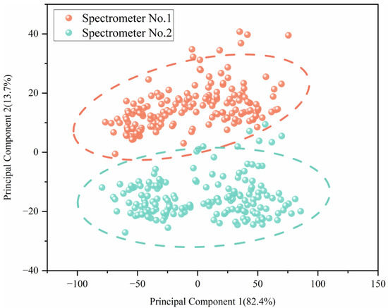
Figure 3.
The PCA chart of spectra from two spectrometers.
3.1.2. Calibration Model Comparison
Firstly, we developed calibration models for each of the two spectrometers to predict total soil nitrogen content, utilizing these predictions as a reference baseline. To facilitate effective calibration model transfer between two spectrometers, we initially preprocessed the spectral data to standardize spectral resolution. Utilizing this preprocessed data from Spectrometer No. 1 and No. 2, we constructed calibration models using three algorithms, PLSR, SVR, and Ridge, to predict soil TN content. The prediction performance of these models is detailed in Table 2.
Table 2.
Prediction performance of soil total nitrogen by PLSR, SVR, and Ridge algorithms on two spectrometers.
Despite notable differences in the spectra, the PLSR model exhibited robust prediction capabilities on both spectra. On the prediction set of Spectrometer No. 1, the model achieved an R2P of 0.779 and an RMSEP of 0.020%, closely matching its performance on Spectrometer No. 2, where it reached an R2P of 0.806 and RMSEP of 0.019%. Both models displayed RPDs exceeding 2.1. Similarly, the Ridge model showed consistency with PLSR under conditions of high covariance [39]. The addition of L2 regularization contributed to model stability, yielding predictive performances of R2P = 0.797 and RMSEP = 0.020% for Spectrometer No. 1, and R2P = 0.795 and RMSEP = 0.020% for Spectrometer No. 2, with both RPDs exceeding 2.2. In contrast, the nonlinear SVR model demonstrated variability in performance due to its sensitivity to the spectral range’s nonlinear features. The SVR model was significantly more effective on Spectrometer No. 2 (R2P = 0.856, RMSEP = 0.017%, RPD = 2.660) compared to Spectrometer No. 1 (R2P = 0.660, RMSEP = 0.025%, RPD = 1.732), indicating Spectrometer No. 2 may contain more nonlinear features, making it more suitable for SVR modeling.
Based on these analyses, we established Spectrometer No. 1 and No. 2 as master and slave, respectively. However, direct model transfer between the spectrometers was found to be unsuccessful based on our preliminary experiments. The significantly low R2P, RPD, and high RMSEP values highlight the profound impact of hardware differences on model performance, indicating the need for further investigation into model transfer techniques to prevent model failure and the necessity for recalibration.
3.2. Standard Calibration Transfer Method
In our study, we designated Spectrometer No. 1 and No. 2 as master and slave, respectively, and employed three calibration transfer methods: DS, PDS, and SST, to modify the spectral data of the slave so that it resembled the spectral morphology of the master. Subsequently, we applied the master’s calibration model to the slave’s prediction set. To assess the effectiveness of these methods, we conducted a comprehensive evaluation, including the average spectral correlation coefficients between the master and slave spectral prediction sets, as well as the performance metrics of the models. This integrated analysis aims to evaluate the feasibility of each calibration transfer method.
The average spectral correlation coefficients between the prediction sets of two spectrometers are presented in Figure 4, demonstrating a significant improvement in correlation when calibration transfer methods are applied. Specifically, with Spectrometer No. 1 as the master and No. 2 as the slave, the correlation of the slave’s transformed data to the master’s data improved markedly—from 0.9566 in untransformed data to 0.9989 for both DS and SST and 0.9988 for PDS. Despite the high performance of the PDS, its spectral correlation was slightly lower compared to DS and SST. This can be attributed to the limitations of the PDS’s moving-window approach, which does not adapt window widths across different wavelengths, potentially reducing the effectiveness of the transformation. Conversely, when roles were reversed with Spectrometer No. 2 as the master and No. 1 as the slave, all three methods effectively enhanced the spectral correlation to the master’s data, achieving coefficients of 0.9995 for both DS and SST and 0.9993 for PDS. This variation highlights how the choice of master and slave influences the effectiveness of the calibration transfer methods.
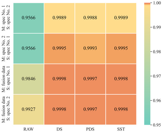
Figure 4.
Average spectral correlation coefficients between the master (M) spectral prediction set and the raw, DS, PDS, SST transformed slave (S) spectral prediction set.
The changes in the predictive performance of the calibration models post-transfer are detailed in Table 3. When Spectrometer No. 1 is the master and No. 2 is the slave, the models, DS-PLSR, PDS-SVR, and DS-Ridge demonstrate significant improvements in predictive performance compared to direct transfer. Specifically, DS-PLSR transitions from an R2P of 0.779, RMSEP of 0.020%, and RPD of 2.149 in the master to 0.545, 0.029%, and 1.497 in the slave. Similarly, PDS-SVR changes from R2P 0.660, RMSEP 0.025%, and RPD 1.732 in the master to R2P 0.497, RMSEP 0.031%, and RPD 1.424 in the slave. DS-Ridge shows a decline from R2P 0.797, RMSEP 0.020%, and RPD 2.244 in the master to R2P 0.540, RMSEP 0.030%, and RPD 1.489 in the slave. Although there is a significant improvement in accuracy compared to direct transfer, the models transferred to the slave still fall short of meeting the requirements for soil TN detection. When Spectrometer No. 2 is designated as the master and Spectrometer No. 1 as the slave, the models DS-PLSR, DS-SVR, and DS-Ridge exhibit strong predictive performance. Specifically, DS-PLSR shows a decrease from an R2P of 0.806 and RMSEP of 0.020% in the master to 0.729 and 0.023% in the slave, with the RPD reducing from 2.233 to 1.940. Similarly, DS-SVR transitions from an R2P of 0.856 and RMSEP of 0.017% to 0.837 and 0.018%, with the RPD decreasing from 2.660 to 2.505. DS-Ridge shows a decline from R2P 0.795, RMSEP 0.020%, and RPD 2.233 in the master to R2P 0.771, RMSEP 0.021%, and RPD 2.111 in the slave. These results demonstrate that when Spectrometer No. 2 serves as the master, there is a relatively minor degradation in model performance post-transfer compared to the scenarios where Spectrometer No. 1 is the master. Notably, the DS-SVR model maintains high predictive accuracy, achieving an RPD greater than 2.5 in the slave configuration. The overall performance of the DS and SST transfer methods are closely matched, with DS marginally outperforming SST. However, PDS achieves optimal results only when combined with the SVR model.
Table 3.
Results of the standard calibration transfer (CT) methods. PDS-PLSR and PDS-Ridge predictions when spectrometer No. 1 is the master and spectrometer No. 2 is the slave are underperforming and are not shown.
These findings underscore that the choice of master and slave spectrometers significantly impacts the effectiveness of model transfer. Although the DS-SVR model exhibits excellent prediction accuracy across both devices when spectrometer No. 2 is used as the master and spectrometer No. 1 is used as the slave, thereby supporting cross-device model generalization, the process of selecting master and slave configurations is both labor-intensive and time-consuming. Furthermore, the results may not always align with specific model transfer requirements. For instance, if the goal is to transfer a model developed on Spectrometer No. 1 to Spectrometer No. 2, the current experimental outcomes may fall short. Additionally, the traditional calibration transfer process encounters increased complexity with multiple spectrometers. As the number of spectrometers grows, so does the complexity of potential master–slave configurations, necessitating numerous experiments. Each additional spectrometer makes the model’s transfer scenarios more complex, complicating the calibration process and making the development of a universally applicable model more challenging. Consequently, there is a pressing need to develop innovative methods that can simplify this process and ensure robust model generalizability across different instruments.
3.3. Data Fusion Combined with Calibration Transfer
In our study, we combined the spectral data from Spectrometers No. 1 and No. 2 to create a master spectrum through a data fusion method, which involved averaging the spectra where each was weighted equally at 50%. The individual spectra from these two spectrometers were then used as the slave spectra. The calibration model established using the master’s fused spectrum was subsequently applied to the slave’s prediction set via three calibration transfer methods: DS, PDS, and SST.
It is shown in Figure 4 that the average spectral correlation coefficients of DS and SST reach 0.9998, and the average spectral correlation coefficient of PDS is slightly lower at 0.9997, indicating a strong similarity between the two transferred slave spectra and the master spectrum. Our fusion approach enhances the calibration transfer outcomes by incorporating characteristics from both slave spectra, thereby minimizing the differences between the master and slave. This is reflected in the performance metrics where the transferred models, utilizing different combinations of DS, PDS, and SST with algorithms like PLSR, SVR, and Ridge, show consistently good results across both spectrometers. The performance disparity observed in previous studies, where the slave’s results significantly lagged behind the master’s, was not evident here. For instance, it is shown in Figure 5 that an R2P of 0.821 and an RMSEP of 0.018% were achieved by the DS-Ridge model on Spectrometer No. 1, which closely aligns with its performance on Spectrometer No. 2, where an R2P of 0.783 and an RMSEP of 0.020% were showcased.
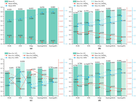
Figure 5.
The prediction performance of the models on the (a) master’s calibration set, and the slave prediction sets after (b) DS, (c) PDS, and (d) SST transformations.
Although the results are promising and balanced across both devices, there is a noticeable decrease in performance compared to the DS-SVR used when Spectrometer No. 2 was serving as the master device, as described in Section 3.2. This indicates a need for further refinement in our calibration transfer approach to enhance model accuracy post-transfer while reducing the labor and resource expenditure associated with selecting different master–slave configurations. Thus, developing a method that both simplifies the master–slave setup and ensures the practical usability of the transferred model is crucial.
3.4. Ensemble Model Transfer
In this section of our paper, we delve into the effectiveness of ensemble model transfer strategies to enhance the robustness and accuracy of model predictions across different devices in soil detection using Vis-NIR spectroscopy. We construct an ensemble stacking model by integrating outputs from three calibration models: PLSR, SVR, and Ridge. This ensemble model aims to leverage the combined strengths of these models to maintain high prediction accuracy and stability during the transfer to a new device.
The ensemble stacking model utilizes PLSR, SVR, and Ridge as its base models, all of which have been previously developed using fusion spectra. The outputs from these base models serve as inputs to a simpler meta-model, multiple linear regression (MLR), to avoid overfitting, as recommended in prior studies [40]. Additionally, we compare MLR with a more complex meta-model, BoostForest, to assess which offers superior transfer performance. Empirical results, detailed in Figure 5, indicate that combining the ensemble stacking method with calibration transfer methods such as DS and SST markedly improves model transfer effectiveness. Both MLR and BoostForest show similar performance levels on the master’s calibration set; however, BoostForest generally provides better results upon model transfer to new devices. For instance, the ensemble model with BoostForest as the meta-model, combined with DS, delivers excellent predictive performance, achieving an R2P of 0.858, RMSEP of 0.016%, and RPD of 2.684 for slave No. 1. For slave No. 2, the performance slightly diminishes, with an R2P of 0.823, RMSEP of 0.018%, and RPD of 2.403. The superior generalization ability of BoostForest, particularly in the context of differing data distributions and feature combinations encountered on different instruments, underscores its utility in ensemble model transfers. While the ensemble model with MLR is effective, the more complex BoostForest model outperforms MLR in most scenarios, demonstrating the potential benefits of using sophisticated meta-models in calibration transfer processes.
However, it is important to note that the effectiveness of the ensemble stacking approach can vary. Poor performance of a single base model or significant discrepancies between the performance of base models can diminish the efficacy of the ensemble model. For example, the ensemble stacking model combined with PDS does not improve the results on both slaves compared to the base model. This underlines the need for careful selection and optimization of base models and their integration strategies to ensure effective model transfer.
In our study, we developed an ensemble stacking model that utilizes DS to enhance prediction accuracy across different devices, referred to as slave No. 1 and slave No. 2. While the model showed promising results on both devices, we observed a significant variance in prediction accuracies between the two. To address this, our objective was to refine the model for more balanced performance across both devices. When the spectra from both spectrometers are equally weighted at 50% for fusion, the model performs better on the test set of slave No. 1. This indicates that the transformation matrix obtained under this weight combination setting can more effectively convert the test set of slave No. 1 into the form of the fused spectrum. To achieve a more balanced result, we attempted to increase the weight of the spectra from slave No. 2 during fusion. We believe that by doing so, the fused spectrum incorporates more characteristics of slave No. 2, making the spectra of the master and slave No. 2 more similar. Consequently, the transformation matrix established between the fused spectrum and slave No. 2 can better convert the test set of slave No. 2 into the fused spectral form. This allows the model built on the fused spectrum to perform more excellently on the transformed test set of slave No. 2. To verify this idea, we set up three groups of fusion weights with increments and decrements of 10%. We tested three different weight combinations: weight combination No. 1: averaging of the two spectra; weight combination No. 2: 40% of spectrometer No. 1’s spectra fused with 60% of spectrometer No. 2’s spectra; and weight combination No. 3: 30% of the spectra of spectrometer No. 1 fused with 70% of the spectra of spectrometer No. 2. The outcomes of these adjustments are illustrated in Table 4. Increasing the spectral contribution from spectrometer No. 2 consistently improved the model’s performance on slave No. 2, albeit at a slight detriment to its performance on slave No. 1. The improvement in the model’s predictive performance on Slave No. 2 when adjusting from weight combination No. 2 to weight combination No. 3 was already very minimal. Therefore, we have set the final results at weight combination No. 3. Weight combination No. 3, which slightly enhanced the model’s predictive accuracy on slave No. 2 without substantially impacting the results on slave No. 1. This adjustment minimized the spectral differences between the master and slave No. 2, facilitating a more effective transformation of slave spectra to the master spectra profile. Consequently, the adjusted model incorporating more features from spectrometer No. 2 displayed improved generalization across the devices.
Table 4.
Effect of adjusting fusion spectral weights on model transfer.
Ultimately, this nuanced adjustment led to an optimized model performance, achieving an R2P of 0.842, RMSEP of 0.017%, and RPD of 2.544 on slave No. 1, and an R2P of 0.830, RMSEP of 0.018%, and RPD of 2.452 on slave No. 2. These results suggest that the model, with adjusted spectral weights, offers a more consistent and generalizable performance across different instruments.
3.5. Discussion
3.5.1. Comparison with Previous Studies
Calibration transfer methods are increasingly adopted in Vis-NIR spectroscopy, notably for measuring soil TN. Typically, the spectrometer that yields the best modeling results is selected as the master, as outlined in Section 3.2 of our study. This choice requires preliminary experiments to determine the most suitable master spectrometer. For instance, one study [41] transferred a calibration model from a standard Vis-NIR spectrometer to a hyperspectral Vis-NIR camera. The model’s performance on the slave device showed an R2P of 0.722 and an RMSEP of 0.399%. Another instance [42] involved multiple instruments, where a laboratory benchtop Vis-NIR spectrometer with superior modeling accuracy served as the master. The model was then adapted to three smaller, less expensive Vis-NIR spectrometers, significantly lowering the cost of soil TN detection. The transferred model achieved RMSEPs of 0.177%, 0.177%, and 0.150% on these devices. In contrast to these approaches, our method eliminates the need to designate master and slave spectrometers. The ensemble stacking model we developed using a master fusion spectrum showed prediction accuracies that were comparable to the aforementioned studies, underscoring the effectiveness of our methodology.
3.5.2. Discussion of Results
Our experimental results demonstrate that using spectrometer No. 2 as the master and spectrometer No. 1 as the slave, the SVR model enhanced by the DS method delivers excellent prediction accuracy on the slave. This outcome underscores that effective model transfer can be achieved by appropriately selecting and pairing the master and slave devices with standard calibration transfer methods. However, achieving the best master–slave configuration requires preliminary independent experiments with each spectrometer, which proves to be both time-consuming and labor-intensive. This complexity runs counter to the primary goal of calibration transfer, which aims to streamline processes. To simplify the calibration transfer and lessen the resource and workload demands, we suggest employing fused spectra as the master spectra. By developing an ensemble stacking model on this master and subsequently transferring it to each slave spectrometer for prediction, we streamline the entire process. Upon adjusting the fusion weights, our method achieved prediction outcomes comparable to those of standard calibration transfer methods across both slave devices. This approach not only enhances efficiency but also maintains high prediction quality.
In practical applications, when dealing with spectra from soil samples with unknown TN content, our method does not require re-creating the fused spectrum using spectral data from both spectrometers and re-modeling on the fused spectrum. Whether using Spectrometer No. 1 or Spectrometer No. 2, after collecting the spectra of the unknown soil samples, the spectra are preprocessed as described in Section 2.2, including interpolation, retaining spectra at 400–2450 nm, and applying SG smoothing. Subsequently, the transformation matrix obtained from our experiments is used to convert the preprocessed spectra. After these steps, the established fused model can be directly applied to predict the TN content of the unknown soil samples. However, our method also has limitations. Due to the limited number and variety of soil samples used for modeling, the representativeness is insufficient, and the spectral features learned by the model are limited. As a result, the model may exhibit poor robustness and decreased performance when dealing with some soil samples.
3.5.3. Research Prospects
From a practical application perspective, we will illustrate the potential application scenarios of our method with examples. In an experimental team, there may be multiple Vis-NIR devices. Our method can achieve parallel measurement across multiple devices. In traditional methods, models need to be established separately based on the spectra of each instrument, which is not only time-consuming and labor-intensive but also results in inconsistent prediction accuracies from multiple models. By establishing a universal model, prediction results can be shared across different devices, improving the efficiency and reliability of measurements. In another scenario, different experimental teams may have laboratory hardware differences, with some only able to purchase low-cost, convenient miniaturized Vis-NIR spectrometers. Models constructed based on spectra collected from miniaturized Vis-NIR devices may be less accurate than those from desktop devices. By applying our method, spectra collected from miniaturized devices can be transformed and used with a universal model for prediction, which helps to improve the detection accuracy of miniaturized devices and facilitates the sharing of Vis-NIR spectral analysis models across different instruments, promoting the dissemination of Vis-NIR devices.
Looking forward, while the establishment of a common model across two spectrometers has demonstrated the potential of our method, we aim to extend this approach to include more spectrometers. This expansion would further test the scalability and applicability of our method in scenarios involving multiple spectrometers. Additionally, although we manually adjusted the weights in the fused spectra to tune the model performance effectively, this process proved to be labor-intensive. Moving forward, we plan to develop an automated weight adjustment mechanism, which could streamline the calibration process and enhance the practical utility of our method in real-world applications. Lastly, in future research, we plan to include a broader variety of soil types to allow the model to learn a wider range of spectral characteristics. This will help us develop a more versatile model with broader applicability.
4. Conclusions
To simplify the traditional calibration transfer process, we introduced a novel approach that utilizes a fused spectrum as the master spectrum. This method involves constructing an ensemble stacking model based on the fused master spectrum and then applying it to predictions for two slave spectrometers using the DS method. Effective predictions of soil TN were achieved, with an R2P of 0.842, RMSEP of 0.017%, and RPD of 2.544 on one spectrometer, and an R2P of 0.830, RMSEP of 0.018%, and RPD of 2.452 on the other spectrometer. Our experimental results validate this approach, showing that it circumvents the need for specific master and slave designations, thereby reducing the effort and resources typically required for master–slave configurations. This method not only simplifies the calibration process but also ensures robust and balanced prediction performance across different spectrometers, achieving effective cross-instrument generalization.
Supplementary Materials
The following supporting information can be downloaded at: https://www.mdpi.com/article/10.3390/chemosensors13020057/s1. Figure S1: Reflectance spectra obtained on both spectrometers; Figure S2: Comparison chart of mean reflectance between the two spectrometers (400–2450 nm). Table S1: The information of the testing agency.
Author Contributions
Conceptualization, Z.T., F.L. and W.K.; methodology, Z.T., X.L., F.L. and W.K.; software, Z.T. and Y.L.; validation, Y.L. and X.L.; investigation, A.T.; resources, A.T.; data curation, Y.L.; writing—original draft preparation, Z.T.; writing—review and editing, F.L. and W.K.; supervision, A.T. and W.K.; project administration, A.T., F.L. and W.K.; funding acquisition, A.T., F.L. and W.K. All authors have read and agreed to the published version of the manuscript.
Funding
This research was funded by the National Natural Science Foundation of China (32371986), the Ningbo Science and Technology Bureau (2024S099), the Science and Technology Department of Shenzhen (CJGJZD20210408092401004), and the Zhejiang Provincial Education Department Scientific Research Project (Y202352714).
Institutional Review Board Statement
Not applicable.
Informed Consent Statement
Not applicable.
Data Availability Statement
The datasets presented in this article are not readily available because they contain proprietary information specific to our research project.
Acknowledgments
The authors gratefully acknowledge the instrumental support provided by Oceanhood Opto-electronics Technology Co., Ltd. (Shanghai, China) and Optosky Technology Co., Ltd. (Xiamen, China).
Conflicts of Interest
The authors declare no conflicts of interest.
References
- Lehmann, J.; Bossio, D.A.; Kogel-Knabner, I.; Rillig, M.C. The concept and future prospects of soil health. Nat. Rev. Earth Environ. 2020, 1, 544–553. [Google Scholar] [CrossRef] [PubMed]
- Bünemann, E.K.; Bongiorno, G.; Bai, Z.; Creamer, R.E.; De Deyn, G.; de Goede, R.; Fleskens, L.; Geissen, V.; Kuyper, T.W.; Mäder, P.; et al. Soil quality—A critical review. Soil Biol. Biochem. 2018, 120, 105–125. [Google Scholar] [CrossRef]
- Grell, M.; Barandun, G.; Asfour, T.; Kasimatis, M.; Collins, A.S.P.; Wang, J.; Güder, F. Point-of-use sensors and machine learning enable low-cost determination of soil nitrogen. Nat. Food 2021, 2, 981–989. [Google Scholar] [CrossRef]
- Fan, Y.; Wang, X.; Funk, T.; Rashid, I.; Herman, B.; Bompoti, N.; Mahmud, M.S.; Chrysochoou, M.; Yang, M.; Vadas, T.M.; et al. A critical review for real-time continuous soil monitoring: Advantages, challenges, and perspectives. Environ. Sci. Technol. 2022, 56, 13546–13564. [Google Scholar] [CrossRef]
- Barra, I.; Haefele, S.M.; Sakrabani, R.; Kebede, F. Soil spectroscopy with the use of chemometrics, machine learning and pre-processing techniques in soil diagnosis: Recent advances–A review. TrAC Trends Anal. Chem. 2021, 135, 116166. [Google Scholar] [CrossRef]
- Ge, Y.; Wadoux, A.; Peng, Y. A Primer on Soil Analysis Using Visible and Near-Infrared (vis-NIR) and Mid-Infrared (MIR) Spectroscopy; FAO: Rome, Italy, 2022. [Google Scholar] [CrossRef]
- Tang, R.; Jiang, K.; Li, C.; Li, X.; Wu, J. Modeling to Correct the Effect of Soil Moisture for Predicting Soil Total Nitrogen by Near-Infrared Spectroscopy. Electronics 2023, 12, 1271. [Google Scholar] [CrossRef]
- Morellos, A.; Pantazi, X.-E.; Moshou, D.; Alexandridis, T.; Whetton, R.; Tziotzios, G.; Wiebensohn, J.; Bill, R.; Mouazen, A.M. Machine learning based prediction of soil total nitrogen, organic carbon and moisture content by using VIS-NIR spectroscopy. Biosyst. Eng. 2016, 152, 104–116. [Google Scholar] [CrossRef]
- Conforti, M.; Castrignanò, A.; Robustelli, G.; Scarciglia, F.; Stelluti, M.; Buttafuoco, G. Laboratory-based Vis-NIR spectroscopy and partial least square regression with spatially correlated errors for predicting spatial variation of soil organic matter content. Catena 2015, 124, 60–67. [Google Scholar] [CrossRef]
- Wan, M.; Qu, M.; Hu, W.; Li, W.; Zhang, C.; Cheng, H.; Huang, B. Estimation of soil pH using PXRF spectrometry and Vis-NIR spectroscopy for rapid environmental risk assessment of soil heavy metals. Process Saf. Environ. Prot. 2019, 132, 73–81. [Google Scholar] [CrossRef]
- Xu, S.; Zhao, Y.; Wang, M.; Shi, X. Comparison of multivariate methods for estimating selected soil properties from intact soil cores of paddy fields by Vis-NIR spectroscopy. Geoderma 2018, 310, 29–43. [Google Scholar] [CrossRef]
- Xu, D.; Ma, W.; Chen, S.; Jiang, Q.; He, K.; Shi, Z. Assessment of important soil properties related to Chinese Soil Taxonomy based on vis-NIR reflectance spectroscopy. Comput. Electron. Agric. 2018, 144, 1–8. [Google Scholar] [CrossRef]
- Liu, Y.; Jiang, Q.; Shi, T.; Fei, T.; Wang, J.; Liu, G.; Chen, Y. Prediction of total nitrogen in cropland soil at different levels of soil moisture with Vis/NIR spectroscopy. Acta Agric. Scand. Sect. B Soil Plant Sci. 2014, 64, 267–281. [Google Scholar] [CrossRef]
- Soriano-Disla, J.M.; Janik, L.J.; Viscarra Rossel, R.A.; Macdonald, L.M.; McLaughlin, M.J. The performance of visible, near-, and mid-Infrared reflectance spectroscopy for prediction of soil physical, chemical, and biological properties. Appl. Spectrosc. Rev. 2013, 49, 139–186. [Google Scholar] [CrossRef]
- Ge, Y.; Morgan, C.L.S.; Grunwald, S.; Brown, D.J.; Sarkhot, D.V. Comparison of soil reflectance spectra and calibration models obtained using multiple spectrometers. Geoderma 2011, 161, 202–211. [Google Scholar] [CrossRef]
- Li, L.; Huang, W.; Wang, Z.; Liu, S.; He, X.; Fan, S. Calibration transfer between developed portable Vis/NIR devices for detection of soluble solids contents in apple. Postharvest Biol. Technol. 2022, 183, 111720. [Google Scholar] [CrossRef]
- Wang, Y.; Veltkamp, D.J.; Kowalski, B.R. Multivariate instrument standardization. Anal. Chem. 1991, 63, 2750–2756. [Google Scholar] [CrossRef]
- Du, W.; Chen, Z.-P.; Zhong, L.-J.; Wang, S.-X.; Yu, R.-Q.; Nordon, A.; Littlejohn, D.; Holden, M. Maintaining the predictive abilities of multivariate calibration models by spectral space transformation. Anal. Chim. Acta 2011, 690, 64–70. [Google Scholar] [CrossRef] [PubMed]
- Fearn, T. Standardisation and calibration transfer for near infrared instruments: A review. J. Near Infrared Spectrosc. 2001, 9, 229–244. [Google Scholar] [CrossRef]
- Li, X.; Pan, W.; Li, D.; Gao, W.; Zeng, R.; Zheng, G.; Cai, K.; Zeng, Y.; Jiang, C. Can fusion of vis-NIR and MIR spectra at three levels improve the prediction accuracy of soil nutrients? Geoderma 2024, 441, 116754. [Google Scholar] [CrossRef]
- Song, J.; Shi, X.; Wang, H.; Lv, X.; Zhang, W.; Wang, J.; Li, T.; Li, W. Combination of feature selection and geographical stratification increases the soil total nitrogen estimation accuracy based on vis-NIR and pXRF spectral fusion. Comput. Electron. Agric. 2024, 218, 108636. [Google Scholar] [CrossRef]
- Breiman, L. Stacked regressions. Mach. Learn. 1996, 24, 49–64. [Google Scholar] [CrossRef]
- Biney, J.K.M.; Vašát, R.; Bell, S.M.; Kebonye, N.M.; Klement, A.; John, K.; Borůvka, L. Prediction of topsoil organic carbon content with Sentinel-2 imagery and spectroscopic measurements under different conditions using an ensemble model approach with multiple pre-treatment combinations. Soil Tillage Res. 2022, 220, 105379. [Google Scholar] [CrossRef]
- Tavakoli, H.; Correa, J.; Sabetizade, M.; Vogel, S. Predicting key soil properties from Vis-NIR spectra by applying dual-wavelength indices transformations and stacking machine learning approaches. Soil Tillage Res. 2023, 229, 105684. [Google Scholar] [CrossRef]
- Pittaki-Chrysodonta, Z.; Hartemink, A.E.; Sanderman, J.; Ge, Y.; Huang, J. Evaluating three calibration transfer methods for predictions of soil properties using mid-infrared spectroscopy. Soil Sci. Soc. Am. J. 2021, 85, 501–519. [Google Scholar] [CrossRef]
- Sanderman, J.; Gholizadeh, A.; Pittaki-Chrysodonta, Z.; Huang, J.; Safanelli, J.L.; Ferguson, R. Transferability of a large mid-infrared soil spectral library between two Fourier-transform infrared spectrometers. Soil Sci. Soc. Am. J. 2023, 87, 586–599. [Google Scholar] [CrossRef]
- Ranger, C.B. Flow injection analysis: Principles, techniques, applications, design. Anal. Chem. 1981, 53, 20A–32A. [Google Scholar] [CrossRef]
- Savitzky, A.; Golay, M.J.E. Smoothing and differentiation of data by simplified least squares procedures. Anal. Chem. 1964, 36, 1627–1639. [Google Scholar] [CrossRef]
- Xu, D.; Chen, S.; Xu, H.; Wang, N.; Zhou, Y.; Shi, Z. Data fusion for the measurement of potentially toxic elements in soil using portable spectrometers. Environ. Pollut. 2020, 263, 114649. [Google Scholar] [CrossRef]
- Kennard, R.W.; Stone, L.A. Computer aided design of experiments. Technometrics 1969, 11, 137–148. [Google Scholar] [CrossRef]
- Wold, H. Soft modelling by latent variables: The non-Linear iterative partial least squares (NIPALS) approach. J. Appl. Probab. 2017, 12, 117–142. [Google Scholar] [CrossRef]
- Sain, S.R.; Vapnik, V.N. The nature of statistical learning theory. Technometrics 1996, 38, 409. [Google Scholar] [CrossRef]
- Hoerl, A.; Kennard, R. Ridge regression: Applications to nonorthogonal problems. Technometrics 1970, 12, 69–82. [Google Scholar] [CrossRef]
- Zhao, C.; Wu, D.; Huang, J.; Yuan, Y.; Zhang, H.T.; Peng, R.; Shi, Z. BoostTree and BoostForest for ensemble learning. IEEE Trans. Pattern Anal. Mach. Intell. 2023, 45, 8110–8126. [Google Scholar] [CrossRef] [PubMed]
- Snoek, J.; Larochelle, H.; Adams, R.P. Practical bayesian optimization of machine learning algorithms. Adv. Neural Inf. Process. Syst. 2012, 25, 2951–2959. [Google Scholar] [CrossRef]
- Chen, L.; Liu, D.; Zhou, J.; Bin, J.; Li, Z. Calibration transfer for near-Infrared (NIR) spectroscopy based on neighborhood preserving embedding. Anal. Lett. 2020, 54, 947–965. [Google Scholar] [CrossRef]
- Ding, J.G.; Li, X.B.; Huang, L.Q. A novel method for spectral similarity measure by fusing shape and amplitude features. J. Eng. Sci. Technol. Rev. 2015, 8, 172–179. [Google Scholar] [CrossRef]
- Chang, C.W.; Laird, D.A.; Mausbach, M.J.; Hurburgh, C.R. Near-Infrared reflectance spectroscopy–Principal components regression analyses of soil properties. Soil Sci. Soc. Am. J. 2001, 65, 480–490. [Google Scholar] [CrossRef]
- Frank, L.E.; Friedman, J.H. A statistical view of some chemometrics regression tools. Technometrics 1993, 35, 109–135. [Google Scholar] [CrossRef]
- Wu, T.; Zhang, W.; Jiao, X.; Guo, W.; Alhaj Hamoud, Y. Evaluation of stacking and blending ensemble learning methods for estimating daily reference evapotranspiration. Comput. Electron. Agric. 2021, 184, 106039. [Google Scholar] [CrossRef]
- Li, X.Y.; Ren, G.X.; Fan, P.P.; Liu, Y.; Sun, Z.L.; Hou, G.L.; Lv, M.R. Study on the calibration transfer of soil nutrient concentration from the hyperspectral camera to the normal spectrometer. J. Spectrosc. 2020, 2020, 8137142. [Google Scholar] [CrossRef]
- Shi, Z.L.; Ren, Z.X.; Yang, Z.L.; Cai, L.W.; Huang, Y.P.; Ge, C.J.; Han, L.J. Deployment strategy of multiple miniaturized near-infrared spectrometers based on spectral transfer for characterizing soil organic matter and nitrogen. Spectrochim. Acta Part A 2024, 320, 124620. [Google Scholar] [CrossRef] [PubMed]
Disclaimer/Publisher’s Note: The statements, opinions and data contained in all publications are solely those of the individual author(s) and contributor(s) and not of MDPI and/or the editor(s). MDPI and/or the editor(s) disclaim responsibility for any injury to people or property resulting from any ideas, methods, instructions or products referred to in the content. |
© 2025 by the authors. Licensee MDPI, Basel, Switzerland. This article is an open access article distributed under the terms and conditions of the Creative Commons Attribution (CC BY) license (https://creativecommons.org/licenses/by/4.0/).