Article

Detection of Harmful H2S Concentration Range, Health Classification, and Lifespan Prediction of CH4 Sensor Arrays in Marine Environments

1
National Key Laboratory of Advanced Micro and Nano Manufacture Technology, Shanghai Jiao Tong University, Shanghai 200240, China
2
Department of Micro/Nano Electronics, School of Electronic Information and Electrical Engineering, Institute of Marine Equipment, Shanghai Jiao Tong University, Shanghai 200240, China
*
Authors to whom correspondence should be addressed.
Chemosensors 2024, 12(9), 172; https://doi.org/10.3390/chemosensors12090172
Submission received: 16 July 2024 / Revised: 14 August 2024 / Accepted: 22 August 2024 / Published: 29 August 2024
(This article belongs to the Special Issue Functional Nanomaterial-Based Gas Sensors and Humidity Sensors)

Abstract

:
Underwater methane (CH4) detection technology is of great significance to the leakage monitoring and location of marine natural gas transportation pipelines, the exploration of submarine hydrothermal activity, and the monitoring of submarine volcanic activity. In order to improve the safety of underwater CH4 detection mission, it is necessary to study the effect of hydrogen sulfide (H2S) in leaking CH4 gas on sensor performance and harmful influence, so as to evaluate the health status and life prediction of underwater CH4 sensor arrays. In the process of detecting CH4, the accuracy decreases when H2S is found in the ocean water. In this study, we proposed an explainable sorted-sparse (ESS) transformer model for concentration interval detection under industrial conditions. The time complexity was decreased to O (n logn) using an explainable sorted-sparse block. Additionally, we proposed the Ocean X generative pre-trained transformer (GPT) model to achieve the online monitoring of the health of the sensors. The ESS transformer model was embedded in the Ocean X GPT model. When the program satisfied the special instructions, it would jump between models, and the online-monitoring question-answering session would be completed. The accuracy of the online monitoring of system health is equal to that of the ESS transformer model. This Ocean-X-generated model can provide a lot of expert information about sensor array failures and electronic noses by text and speech alone. This model had an accuracy of 0.99, which was superior to related models, including transformer encoder (0.98) and convolutional neural networks (CNN) + support vector machine (SVM) (0.97). The Ocean X GPT model for offline question-and-answer tasks had a high mean accuracy (0.99), which was superior to the related models, including long short-term memory–auto encoder (LSTM–AE) (0.96) and GPT decoder (0.98).

1. Introduction

Marine combustible ice is an ideal energy source for low-carbon societies [1,2,3] because its combustion produces ten times more energy than gasoline, coal, or natural gas [4,5,6,7]; so, coastal countries compete to develop combustible ice resources. Methane (CH4) gas formed after the mining of marine combustible ice can be transported by laying submarine pipelines, and pipeline safety monitoring has become an important work during transportation. Once the CH4 pipeline leaks, it will not only cause damage to the natural environment but also directly affect the energy supply problem and even cause social panic. Therefore, it is of great theoretical value and practical significance to strengthen research on underwater CH4 sensor arrays technology [8,9] and solve technical problems such as underwater CH4 pipeline leakage monitoring and positioning. In addition, hydrothermal activities of submarine “hot springs” and submarine volcanic activities will also release CH4 gas, and the monitoring of the CH4 information also requires underwater CH4 sensor arrays. In the process of underwater CH4 detection, hydrogen sulfide (H2S) gas is often present, which is harmful for the performance of the CH4 sensor [10,11] and seriously affects the health and life of the CH4 sensor arrays.
H2S gas and other sensors’ fault situations affect CH4 detection accuracy [12,13,14,15,16]. To study whether or not the CH4 sensor works properly, the accurate concentration of H2S gas in the external environment should be determined at first. Different concentrations of H2S gas have different effects on CH4 sensor poisoning; therefore, the different levels of H2S gas poisoning can assess the risk of the detection mission and promote the smooth execution of the mission. To detect the working conditions of sensor arrays, health management decision-making is essential. A solution must be established to ensure that the health status of all sensors in the system is clear and that the system is stable.
Data acquisition, failure detection and diagnosis, failure recovery and prediction, health evaluation, and maintenance decision-making are featured in the prognostics and health management (PHM) decision synthesis technique [17,18,19,20]. The reliability and safety of these systems can be enhanced for the purpose of making health management decisions [21,22,23,24]. According to collected data, a system’s health status can be predicted and evaluated to make more informed health management decisions [25,26,27,28]. Previous research has been used to complete these types of health evaluations and to monitor conditions [29,30,31,32]. On the basis of this theory and technical applications in previous work, the current health management decision-making method can be divided into three categories: data-based maintenance decision-making, model-based maintenance decision-making, and reliability-based decision-making [25,26,27,28,33]. The environment has a significant effect on sensor systems, which have changeable working conditions and complex structures. Because the baselines of the same concentrations change at various times, the failure range is hard to define. Therefore, to maintain suitable decision-making conditions for these sensor systems, it is essential to develop appropriate models.
D–S evidence theory [33,34,35], Bayes theory [36,37,38,39], and fuzzy set theory [40,41,42,43,44], as the traditional reliability-based methods, have faced significant challenges because of the various data types and information uncertainty. Conflicting evidence has caused results from the D–S evidence theory to differ from the user’s understanding. Using the D–S evidence theory to address conflicting results under system failure remains challenging. The basis of Bayes theory method is prior probability. When a prior probability is known, it is easy to obtain accuracy results; however, when a prior probability is not known, it is difficult to obtain, and the ability to apply this information is limited. When considering maintenance decision-making tasks, because of the logical reasoning of fuzzy set theory, several subjective factors can affect the description of information. As a result, objectivity in the representation and processing of this information will be lacking.
In this study, we found that it was difficult to apply these maintenance decision-making methods. Shen et al. [31] proposed multifunctional sensor health reliability to assess the working state of the sensor. The quantitative description of health information is called health reliability (HRD). The failure of a single sensor was not effectively revealed when too many sensors were used [32]. To enhance the poison concentration, residual life, and health-level information of the sensor’s health, we developed a nested intelligent health management and life prediction system.
An explainable sorted-sparse (ESS) transformer model was proposed for toxic gas concentration interval detection of CH4 sensor arrays in ocean conditions. The proposed model is a data-based supervised-learning method, requiring label data for training and presenting high accuracy for industrial promotion and application. The time complexity can be decreased to O (n logn) using the ESS block. In addition, we propose the Ocean X generative pre-trained transformer (GPT) model for intelligence health management and lifetime prediction of CH4 sensor arrays by embedding the GPT model with ESS transformer models. The proposed model provides a substantial amount of expert information about sensor array failures and electronic noses by text and speech. This concept also used a question-and-answer system framework.
(1)
To limit the time complexity to O (n logn), we changed the traditional self-attention mechanism to ESS attention. The proposed model used the idea of sorting the product weights of the query and the key value from high to low. Using the original distribution of the training data, we retained the first third and sparse the rest with an explainable mask.
(2)
We enhanced the attention of the Ocean X GPT model with a Rotary Position Embedding (RoPE) attention mechanism. This attention not only had RoPE position information but also retained the original information. Applying the idea of a residual network, we added the original data to the query and key, which were mapped by RoPE. Then, we mapped the total return data into the RoPE again. For the question-and-answer task, the model obtained the position information between the question and the answer from the first RoPE operation. Then, we increased the accuracy of the answer according to the second RoPE operating by combining the question and the target answer.
(3)
We proposed a real-time interactive health management and life prediction system. The basic framework was the Ocean X GPT model with an ESS transformer model embedded inside. When performing the task, according to the keyword in the question, the program jumped into the ESS transformer model and waited for input data. After we entered random validation data x into the trained toxic gas concentration interval detection model (ESS transformer), the model returned the corresponding concentration information, poisoning grade, and remaining life information as a voice broadcast.

2. Theoretical Fundamentals

2.1. ESS Mask

Figure 1 shows the proposed method, which was the result of the ESS mask of temporal and spatial dimensions in a factorized self-attention model [45]. We called the proposed factorized attention “fixed attention”, as shown in Figure 1a. Fixed attention has two mechanisms (FA1 and FA2), where FA1 represents the triangular region (light blue), and FA2 represents the vertical fixed region (sky blue) with L-separated distances. For each current token (deep blue), it is possible to traverse to its left (light blue) until encountering the first token selected by FA2 (sky blue). We called the factorized attention “strided attention”, as shown in Figure 1b. Strided attention has two mechanisms (SA1 and SA2), where SA1 represents the galaxy-shaped region (light blue), and SA2 represents the hackly bar-shaped region (sky blue). In SA1, each token can focus only on the L tokens adjacent to the left. In SA2, each token can focus only on the token to its left. We selected these attended tokens by counting them to the left of their position, and there was one token for every L. L equaled 3 from the original model. Based on this model and the decoder mask shown in Figure 1c, we proposed the explainable sorted–fixed mask shown in Figure 1d.
To map a matrix of input embeddings X to an output matrix, we used a self-attention layer. We parameterized this layer according to a connectivity pattern T = { T 1 ,   ,   T n } , where Ti is the set of indices of the input vectors to which the ith output vector attends. We used a weighted sum of transformations of the input vector for the output vector, as follows:
A t t e n d X ; T = a x i ; T i i ϵ 1 ,   ,   l
where a ( x i ; T i ) denotes the traditional attention score; T i = { j : j i } denotes the full self-attention for autoregressive models, which enabled each element to attend to its own position as well as each of the previous positions.
More precisely, the set Ti is divided into p non-overlapping subsets, and the subset m is represented as A i ( m ) T i , m = 1 , , p ; so, the maximized path of the output situation i and random j is p + 1. For example, if (j, c, d, e, …, i) is the index path of i and j, j A c 1 , c A d 2 , d A e 3 .
We defined the two sparse patterns shown in Figure 1d: (1) one head attended to the previous l locations, and (2) the other head attended to every lth location, where l reflects the stride and was close to n (called “strided attention”). If the data had a structure that was naturally aligned with the stride (e.g., some types of music), this proved to be a convenient formula. For Equation (2), l = 6 corresponds to the number of sensor arrays:
A i ( 1 ) = k , k + 1 , , i
where k is the maximum of (0, il).
A i ( 2 ) = j : ( i j )   m o d l = 0
For the second pattern called “fixed attention”, we propagated the summary of previous locations to all future cells as follows:
A i ( 1 ) = j : j l = j l ,   w h e r e   k = max 0 , i l
where k denotes the maximum of (0, il).
A i ( 2 ) = j : j   m o d   k k c , , k 1
where c is a hyperparameter.
In fixed attention, it is important to pay attention to tokens in other locations regardless of the current token location. This kind of attention gives more attention to the global weight information, where c = 5 corresponds to the number of sensor arrays.
Another concept of this sparse mask includes the probability distribution information of the device array data used in this study, which required a tedious derivation of its formula to verify results (see Section 2.2).

2.2. ESS Attention

Inspired by the prob-sparse self-attention mechanism from Informer [45], we apply ESS attention as our basic model. We observed the same relationship between function detection and self-attention with the prob-sparse self-attention mechanism (see details in Supplementary Materials).
The original attention can be defined as follows:
A q i , k , v = j k q i , k j l k q i , k l V j = D p k j | q i V j
where p ( k j | q i ) = k ( q i , k j ) / l k ( q i , k l ) , and k ( q i , k j ) selects the asymmetric exponential kernel exp q i , k j T / n .
We proposed the max-mean measurement to replace the previous methods. The specific proof method is given in the Supplementary Materials. Calculating the sparsity score for each query would result in additional computation, and that assumption can present the dot-product results following a long-tail distribution. Therefore, each query sparsity score can be calculated with only some of the sampled keys. Therefore, under the long-tail distribution, it was only necessary to compute M by randomly sampling the set of dot-product pairs and by filling the other pairs with 0 values. Sparse Top-U was selected as Q; and for M, the max-operator was stable and insensitive to 0.
N ¯ q i , k = max j q i , k j T d 1 L K j = 1 L K q i , k j T d
d e f max j { q i , k j T } mean j { q i , k j T }
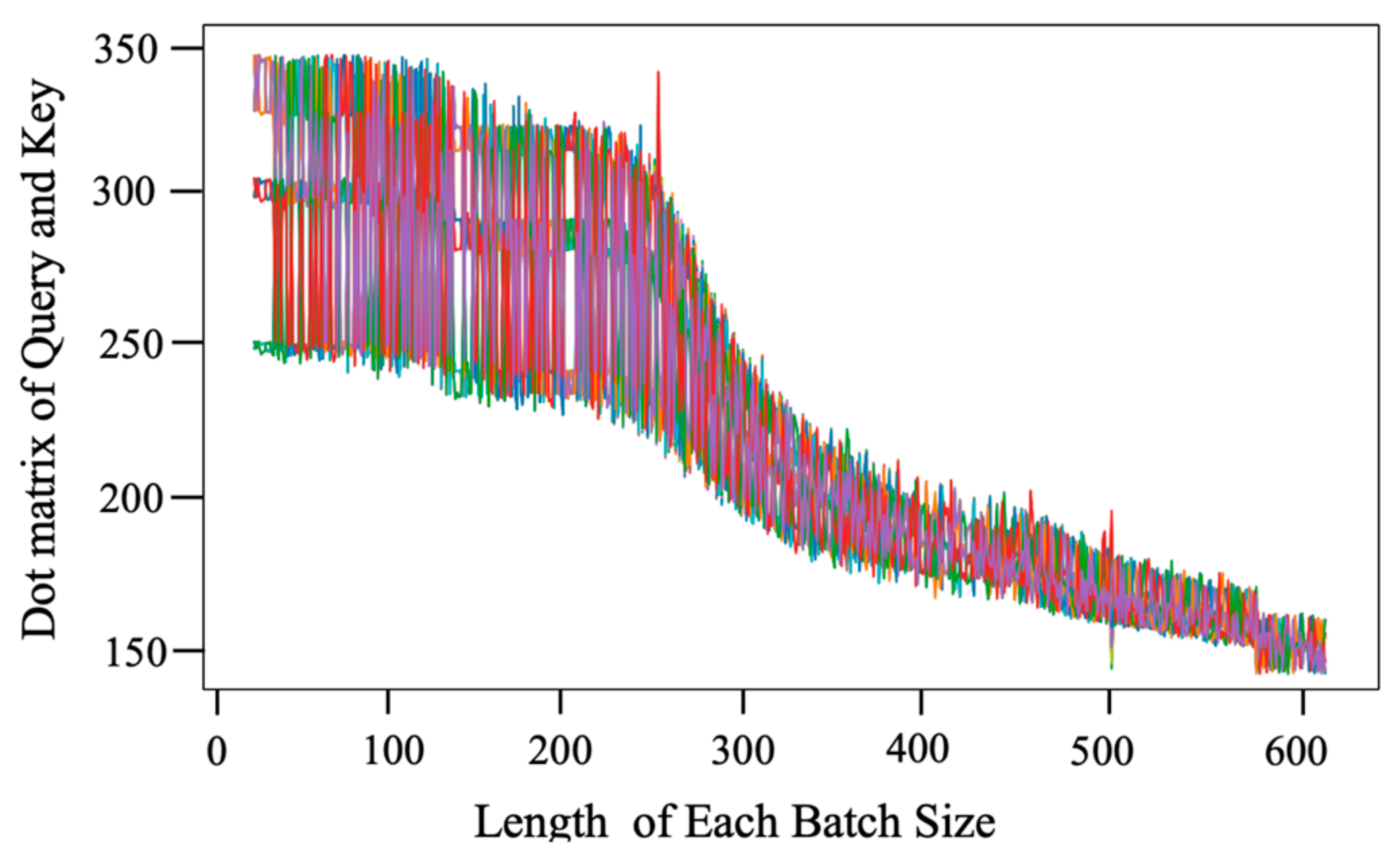
According to the max-mean method, the result of multiplying the query and key matrix is shown in Figure 2. From Figure 2, the total data were N ¯ q i , k , where i is from 1 to 607. By comparing the results shown in Figure 2 with the following data, we observed that the first third of the data had a larger value range, which helped the model distinguish among the different types of data. This distinction information among different classifications was mostly in this area. Therefore, we only kept the first third and took the average value later. Compared with Figure 1d, we retained one-third of the whole 25 × 25 mask.
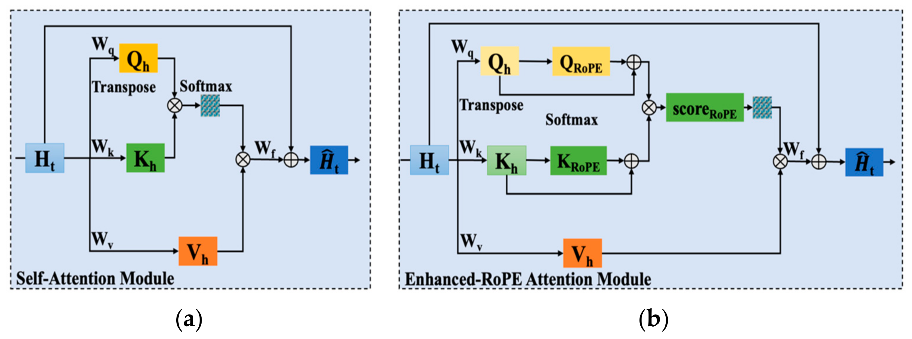
We identify a significant difference between the original and proposed models (Figure 3). Specifically, the matrix product of the query and key matrix did not directly calculate the score. We first multiply Q by the sorted-sparse mask and then by K, thus limiting the time complexity to O (n logn). The pseudocode of ESS attention is given in Algorithm 1.
Algorithm 1 ESS Attention
FunctionESS Attention (Xinput)
Q, K ← Xinput
Q ,   K   (Batch, Head, 608, 25)
K ← Randint (len(X) = 25)
QK_sample ← Q ∗ K
M_top ← Sort (QK_sample)
Visualized (M_top)
QSortedSparse ← Q ∗ Mask
Score = QSortedSparse ∗ KT
End
For the QK_sample, the output is as follows:
Q K s a m p l e = Q K
where Q and K are from the Xinput.
Then, the sorted of QK_sample is as follows:
S o r t e d Q K s a m p l e = N ¯ q i , k
where i is from 1 to 607.
The visualization of M_top is shown in Figure 2. After analyzing the information in Figure 2, we confirmed that only the first third of the data was taken. We combined it with the ESS mask, and then we made the last mask. The sorted-sparse query is as follows:
Q s o r t e d   s p a r s e = Q m a s k

2.3. Enhanced Rotary Positional Embedding Attention

Typically, using a self-attention mechanism, the position information of individual tokens can be leveraged through the use of transformer-based language modeling [46]. On the basis of this original mechanism, q m T k n typically allows for knowledge to be shared among tokens at various locations. To add the relative location information, we used a function g to formulate the inner product of query qm and key kn, which considered their relative position m − n and the word embeddings xm, xn as the input variables. We proposed the inner product to encode only the relative form of the location information as follows:
f q x m , m , f k ( x n , n ) = g ( x m , x n , m n )
To solve the functions fq (xm; m) and fk (xn; n), we looked to align the previous relationship using a similar encoding mechanism.
We used a dimension d = 2 to define a simple case. Accordingly, we used a two-dimensional (2D) plane for the geometric property of the vectors as follows:
f q x m , m = W q x m e i m θ
f k x n , n = ( W k x n ) e i n θ
g x m , x n , m n = R e [ W q x m W k x n e i ( m n ) θ ]
where Re[·] denotes the real part of a complex number; (Wk xn)* denotes the conjugate complex number of (Wk xn); and θR denotes a preset nonzero constant. We then calculated f{q, k} in a multiplication matrix as follows:
f { q , k } x m , m = c o s   m θ s i n   m θ s i n   m θ c o s   m θ W q , k 11 W q , k 12 W q , k 21 W q , k 22 x m 1 x m 2
where ( x m ( 1 ) , x m ( 2 ) ) is the expression of xm in the 2D coordinates; g denotes the matrix and solves Equation (11) under the 2D case. Specifically, the relative position embedding was straightforward: we rotated the affine-transformed word-embedded vector according to the number of angle multiples of its location index and thus interpreted the RoPE intuition.
To simplify the 2D results to any x i R d , where d is even, we divided the d-dimension space into d/2 subspaces and combined them in the merit of the linearity of the inner product, transforming f{q, k} as follows:
f { q , k } x m , m = R Θ , n l W q , k x m
where the rotary matrix with preset parameters Θ = { θ i = 10,000 2 i 1 d , I [ 1 , 2 , , d / 2 ] } is as follows:
R Θ , n l c o s   n θ 1 s i n   n θ 1 0 0 0 0               s i n   n θ 1 c o s   n θ 1 0 0 0 0               0 0 c o s   n θ 2 s i n   θ 2 0 0                 0 0 s i n   n θ 2 c o s   n θ 2 0 0                                           0 0 0 0 c o s   n θ l / 2 s i n   n θ l / 2               0 0 0 0 s i n   n θ l / 2 c o s   n θ l / 2
The original attention can be represented as follows:
q m T k n = R Θ , m l W q x m T R Θ , n l W k x n = x T W q R Θ , n m l W k x n
where R Θ , n m l = ( R Θ , m l ) T R Θ , n l .
For a computationally efficient realization of the multiplication of R Θ l and x R d , we took advantage of the sparsity of R Θ , n l in Equation (15) as follows:
R Θ , n l   = x 1 x 2 x 3 x 4 x l 1 x l         c o s   n θ 1 c o s   n θ 1 c o s   n θ 2 c o s   n θ 2 c o s   n θ l 2 c o s   n θ l 2         +         x 2 x 1 x 4 x 3 x l 1 x l         s i m   n θ 1 s i m   n θ 1 s i n   n θ 2 s i n   n θ 2 s i n   n θ l / 2 s i n   n θ l / 2
The RoPE principal formula derivation and the relationship with relative position embedding are given in Figure S1. According to the RoPE mechanism, we proposed an enhanced-RoPE mechanism in our model to improve the question-and-answer position information to increase accuracy. The enhanced-RoPE attention is shown in Figure 4.
As shown in Figure 4, we proposed an enhanced-RoPE mechanism. The specific operation applied the residual network. To solve the problem of gradient explosion and disappearance with an increase in the number of model layers, we developed the residual network. Image processing and other traditional neural networks often feature a lot of pooling and convolutional layers. Because each layer extracts features from the previous layer, degradation generally occurs as the number of layers increases and other problems emerge. To avoid these types of problems caused by deep neural networks, we adopted the jump connection method for the residual network, which we defined as follows:
y = F x , W i + x
where y denotes the output of the module, x denotes the input of the module, and F x , W i represents the learned residual mapping.
We multiplied x by a linear map Ws so that F and Ws x had the same dimension in Equation (18).
y = F x , W i + W s x
The identity mapping mitigated the degradation problem and could be simple, where Ws is used only to match the dimension of x. In this study, we used a one-layer residual network that was similar to a linear fully connected layer residual network. Algorithm 2 shows how it works.
Algorithm 2 Enhanced-RoPE Attention
FunctionEnhanced-RoPE Attention (Xinput)
Q, KXinput
QRoPE R θ , n l · Q, KRoPE R θ , n l · K
Score = (QRoPE + Q) ∗ (KRoPE + K) T
ScoreRoPE R θ , n l ·Score
End
In Algorithm 2, we first applied something like a residual network to the query and key entered into the RoPE:
Q R o P E = x W q R Θ , m l
K R o P E = x W k R Θ , n l
We added operations like residual networks to Q R o P E and K R o P E . Then, we calculated the score of attention:
S c o r e = F x q , W i + W s x q F x k , W j + W s x k T
where F x q , W i ,   x W q R Θ , m l , and x W k R Θ , n l , respectively.
We operated RoPE operation again on the score. The ScoreRoPE was proposed to be combined with the Value as follows:
S c o r e R o P E = x s c o r e W s c o r e R Θ , n m l

2.4. Ocean X GPT Question-Answering System with Embodied Intelligence

Decoder: A stack of identical layers (N = 3) was included in the decoder. The decoder inserted a third sublayer as well as two sublayers in each encoder layer. This enabled the decoder to perform multi-head attention over the encoder stack’s output. Around each sublayer, we employed residual connections followed by layer normalization, similar to the encoder. For the structural part of the model, see the legend in the Supplementary Materials.
Algorithm 3 shows the Ocean X GPT question-and-answer system with embodied intelligence.
Algorithm 3 Ocean X GPT Question-and-Answer System with Embodied Intelligence
          Question ← “Input:”
          While True:
                              temp_sentence == input (“…”)
                              Question ← temp_sentence
          If Question == “The environment outside”
          |   b ← model. Predict (XRandom_inside). Argmax (−1)
          |   If b == 0:
          |     | a == “answer 0”
          |   elif b == 1:
          |    |               a == “answer 1”
          |   elif b == 2:
          |     |              a == “answer 2”
          |   elif b == 3:
          |      |   a == “answer 3”
          else a ← GPT.answer (Question)
Return a
Algorithm 3 integrates the concept of embodied intelligence into the system. Based on the data collected by the external sensor, it broadcasts the working status and environment of the sensor in real time. This function’s health management concept made strong engineering sense.
The proposed health management system was based on a question-and-answer dialog model. First, we entered the questions into the model in text form. When the content of questions contained the “outside environment”, the model would jump into the ESS transformer model and return the output result based on the external data. Because the input result in this part was random, we created dynamic data, which could be combined well with various situations under real working conditions. The sensor arrays would know the corresponding gas concentration and remaining working time according to external data by the pre-training model. These judgments enabled the sensor arrays to make corresponding decisions and create embodied intelligence. When the question did not contain the keywords (e.g., the “outside environment”), the model would output the question in the form of a voice broadcast according to the trained offline question-and-answer corpus, which helped the questioner learn the knowledge of the deep-sea CH4 detection.

2.5. Encoder and Decoder Stacks

Encoder: A stack of identical layers (N = 4) was included in the encoder for the toxic gas concentration detection task shown in Figure S2a. All layers had two sublayers. The first layer featured a multi-head sorted-sparse attention mechanism. The second layer featured a simple, position-wise fully connected feed-forward network. We employed a residual connection to surround each sublayer after layer normalization. Each sublayer output was Layer–Norm (x + Sublayer(x)), where Sublayer(x) was implemented by the sublayer. All model sublayers, as well as the embedded layers, produced outputs of dimension dmodel = 16 to facilitate these residual connections.
Decoder: A stack of identical layers (N = 6) was included in the decoder for the Ocean X GPT model shown in Figure S2b. In each encoder layer, the decoder had a third sublayer in addition to the two sublayers. This encoder applied multi-head attention over the encoder stack’s output. We used residual connections around the sublayers like the encoder after layer normalization. Table S1 lists parameters used in the interval detection task for toxic gas concentration. We considered the complexity of the toxic gas data and decreased the parameter head to three to ensure that sufficient attention was provided to determine the relationship among data in the training process. We used the classic transformer model without changes in the middle layer. To avoid overfitting during training, we used the dropout operation in Layers 3 and 4, which caused the test set to perform poorly. Table S2 lists the parameters used in the Ocean X GPT model. We set the number of layers to six and the parameter head to eight.

3. Experiment, Results and Discussion

3.1. Setup of Experiment

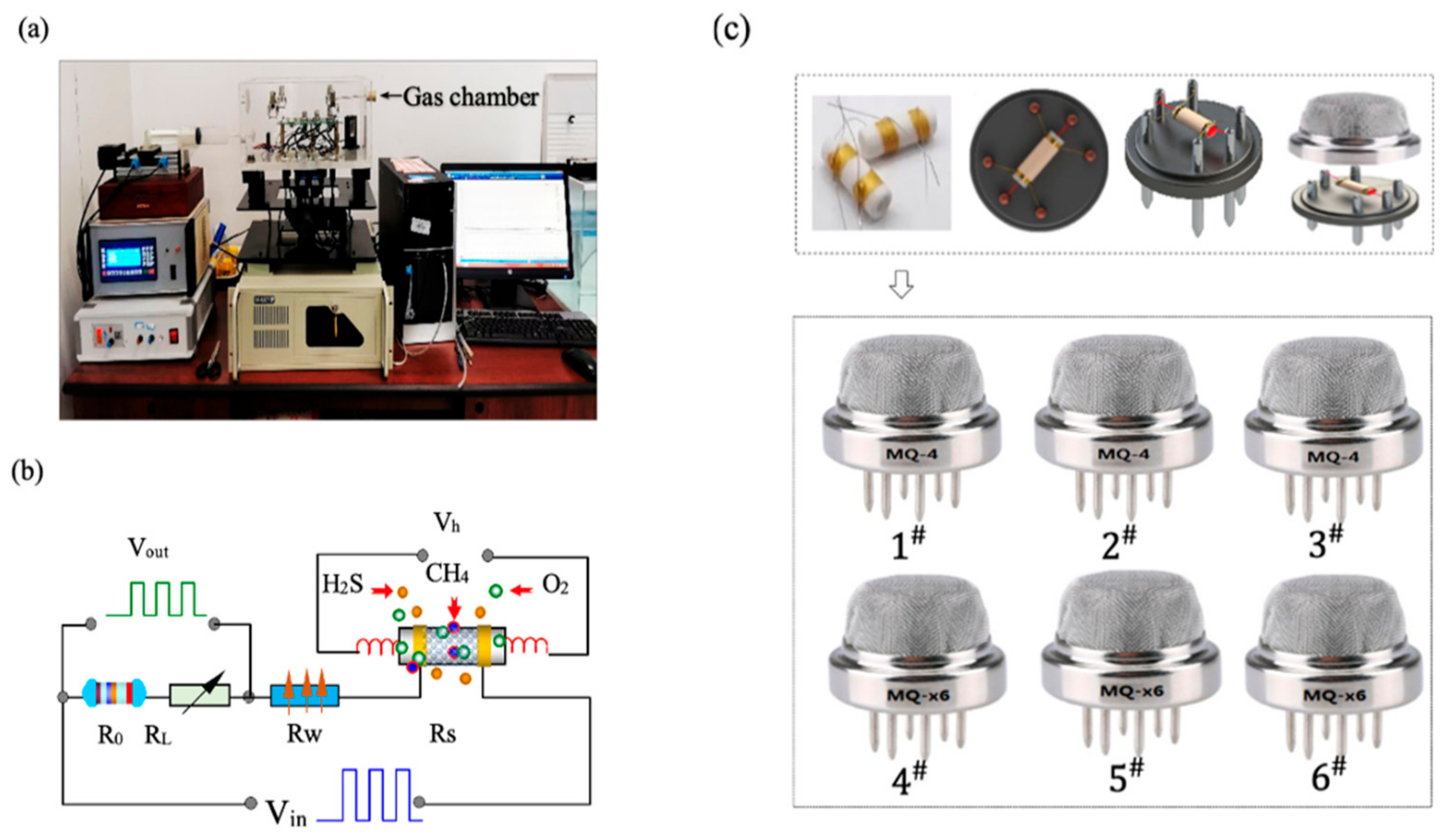
The experimental system provided all the data in this study. Figure 5a illustrates the CH4 sensor array diagram. This experimental system featured the following six parts: (1) the air chamber and gas circuit parts, (2) the communication module, (3) the host computer, (4) the air path, (5) the air chamber, and (6) the environmental stress simulator. The vibration stress amplitude ranges from ±1.5 mm and the frequency ranges from 0 to 120 Hz. The angle range of the sway stress was ±15°. The temperature increase ranged from 0 to 10 °C.
After testing and training, the sensor array studied in this paper will be installed on the underwater robot, and the underwater methane detection will be carried by the robot. In practical engineering, the robot is driven by a propeller, and the propeller is controlled by a motor. When the motor works, it will produce vibration stress (noise) in a certain frequency range. We use the vibration motor to load it on the gas chamber to simulate the vibration stress generated by the robot working, with amplitude ±1.5 mm and frequency 0–120 Hz. When diving, the impact of ocean current will also cause the underwater robot to sway. We use the sway motor to pull the gas chamber sway to simulate the robot sway, and the sway Angle is ±15°. The temperature of sea water will also change. A heating wire is installed in the gas chamber as a heater to make the temperature change in the gas chamber to simulate the change in an underwater temperature environment. The change in the temperature environment is 0–10 °C.
Loading environmental factors, such as vibration, sway, and heating, into the test enables the examination of whether the sensor array can work normally and fail under complex working conditions. Due to the applied vibration and sway stress, although it will cause periodic interference to the sensor array, the interference signal is superimposed on the sensor output and has little impact on the detection accuracy, so it is not discussed in detail. In addition, the heating factor is loaded into the test, which is also to examine whether the sensor array can work normally under variable temperature conditions. Although the applied temperature stress will also cause interference to the sensor array, the normal working temperature of the sensor is about 450 °C, and small temperature changes will not have a great impact on the detection accuracy, so this paper does not focus on the analysis.
The sensing transmitter is composed of a sensing resistor RS, a fixed sampling resistor R0, an adjustable potentiometer RL, a programmed potentiometer RW, a heating voltage Vh, and a working voltage Vin. Two-way communication and data transmission enabled communication with the host computer. The primary platform of the test system was the host computer. It sent down control commands and received temperature, air pressure, humidity, sway, vibration, and gas concentration detection information from the communication module. It also collected output signals from the sensor arrays and extracted characteristic information. Figure 5b shows the sensor signal pickup circuit structure. Figure 5c shows the MQx6 and MQ4 gas sensor cylinder core structure. Pattern recognition is realized by using a 2 × 3 array composed of two types of sensors: MQx6 and MQ4. We used Windows 10 on a 2.8 GHz Intel CPU with 16 GB RAM.
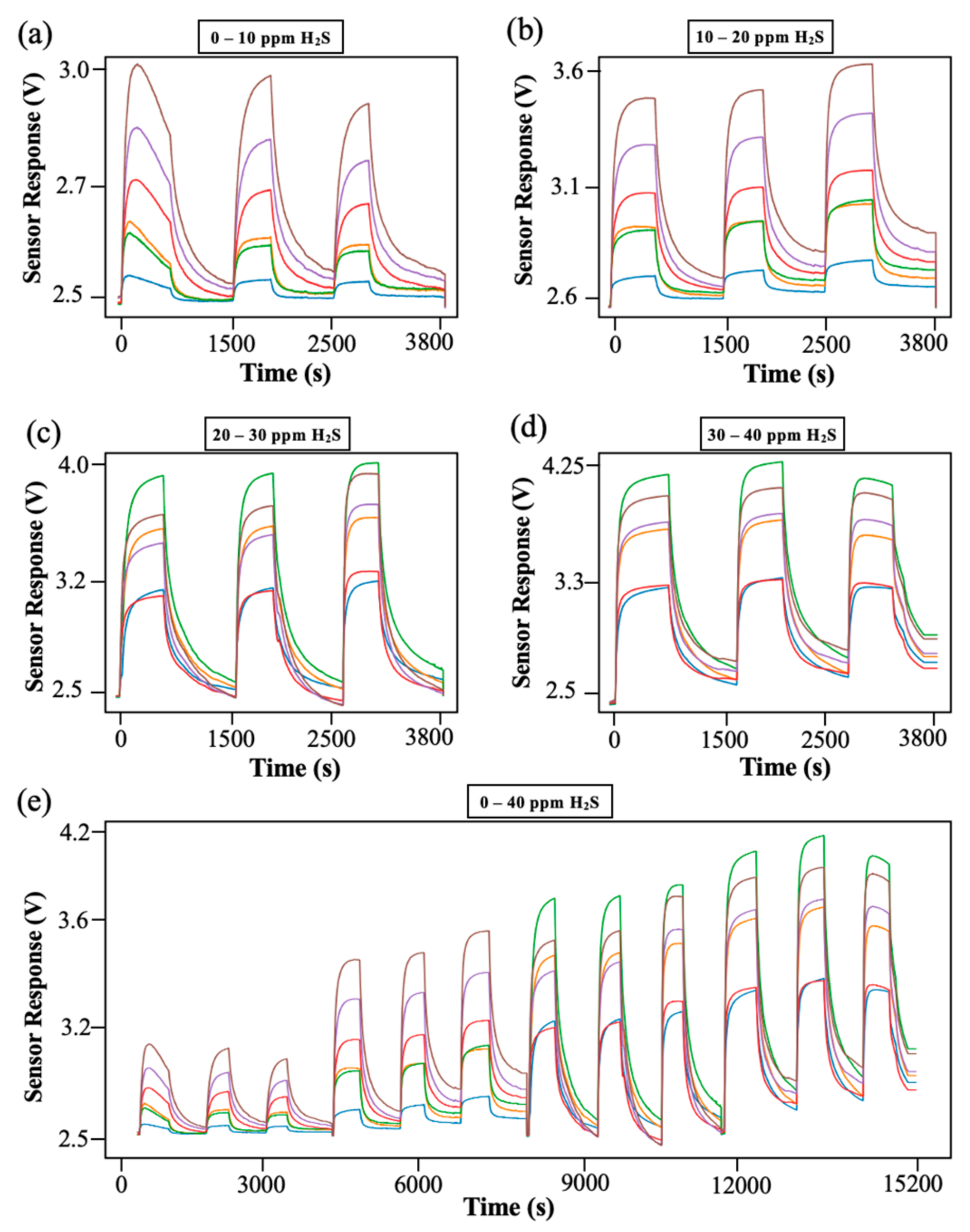
In this research work, the gas static test method is used, and the experimental system in Figure 5a is used for gas concentration test. The specific method is to use the standard air bag to take high-purity (99.99%) H2S Gas and high-purity (99.99%) CH4 gas, and then use the standard syringe to take the measured gas from the air bag and inject it into the air chamber of the experimental system so that the standard concentration of H2S gas and standard concentration of CH4 gas can be prepared. Then, the experiment of the methane sensor array placed in the air chamber is realized. The designed volume of the air chamber used in our test is 13.6 L. Under normal circumstances, the air chamber is filled with air. Since the consumption of O2 is very small in the test process, it can reach a degree of neglect, so the influence of O2 is not deeply discussed in this paper.The yellow, green, and blue curves are MQx6 sensors; purple, red, and brown are MQ4 class sensors. A 2 × 3 sensor array is formed. Figure S3 shows the relationship of toxic gas concentration interval detection.
In Figure 6a, the hydrogen sulfide concentrations are 8 ppm, 6 ppm, and 4 ppm. In Figure 6b, the hydrogen sulfide concentrations are 14 ppm, 16 ppm, and 18 ppm. In Figure 6c, the hydrogen sulfide concentrations are 24 ppm and 25 ppm. In Figure 6d, the hydrogen sulfide concentrations are 35 ppm, 38 ppm, and 34 ppm. The methane background concentration is 10 ppm (8 ppm). The sensor array consists of three MQ4 sensors and three MQx6 sensors. For methane gas, the sensitivity of the MQ4 sensor is higher than that of the MQx6 sensor. For H2S gas, the sensitivity of the MQx6 sensor is higher than that of the MQ4 sensor.

3.2. Flowchart of Question-and-Answer Health Management Systems with Embodied AI

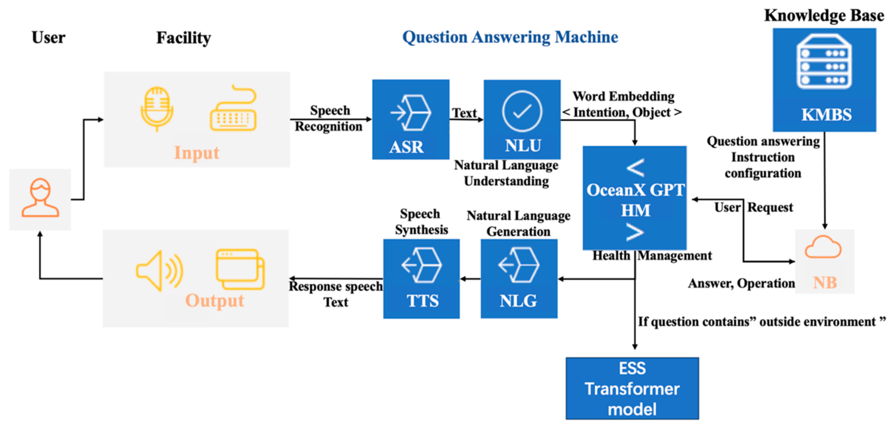
To develop the Ocean X GPT model, we created an AI model based on multi-sensor data under changing operating conditions to support a question-and-answer health management system. Figure 7 shows the experimental method’s flowchart.
The health management process featured the following three steps:
Step 1: For the input, the model used the voice signal from the user and converted it to a text signal, which was entered into the trained model to be processed. Some of these previously designed questions contained the external environment information, and the corresponding answers to these questions had an impact on the working instrument. Based on the sensor array information that was returned, we observed the current external environment information. According to the trained ESS transformer model, we calculated the health condition and remaining working time of the machine, which enabled the corresponding engineering decisions. This concept of making hardware decisions through software algorithms is called embodied AI.
Step 2: In the Ocean X GPT health management section, the model translated text into machine language by word embedding. The model iterated the corresponding answer through the information from the knowledge base. When the problem included the keyword “external environment, etc.”, it jumped to the ESS transformer model to return the value y. The operation of connecting the ESS transformer model and Ocean X GPT model enabled the health management system to be an online monitoring system. Each x entered the model randomly, which simulated the random situation in a real working condition and returned the corresponding y value, which corresponded to the answer for that health management level.
Step 3: In the answer part, the model converted the answer into text by NLG, and then converted it into speech through speech synthesis to complete the broadcast. We used python’s speech-to-text conversion plug-in to implement the dialog system. The machine also provided feedback to the answer for the user through a voice broadcast, which replicated human–computer interaction.

3.3. Validation of Anomaly Detection Method and Inference

3.3.1. Toxic Gas Concentration Interval Detection Evaluation Metrics

We evaluated metrics of the toxic gas concentration interval detection methods. We used precision rate in Equation (23), recall rate in Equation (24), F measure in Equation (25), and accuracy rate (Acc) in Equation (26):
P r e c i s i o n = T P T P + F P
R e c a l l = T P T P + F N
F 1 s c o r e = 1 + x 2 × P r e c i s i o n × R e c a l l α 2 × P r e c i s i o n × R e c a l l
A c c = T P + T N T P + T N + F P + F N
where FP and FN are the false positives and false negatives, respectively. TP and TN are the true positives and true negatives, respectively, and α = 1.
For indicators of model performance, we adopted the mean squared error (MSE), mean absolute error (MAE), and root mean squared error (RMSE) of the predicted and true targets. For MAE, MSE, and RMSE, the corresponding calculations are given in the following equations:
M A E = 1 n i = 1 n y _ t e s t y p r e
M S E = 1 n i = 1 n y _ t e s t y _ p r e 2
R M S E = 1 n i = 1 n y _ t e s t y _ p r e 2
where y pre denotes the predicted tool wear value in the dataset, y test represents the true tool wear value in the dataset, and n is the number of test samples.

3.3.2. ESS Transformer Toxic Gas Concentration Interval Detection Results and Discussion

We trained 50 iterations in the ESS transformer model. We set the batch size to two in the training process. We set the dynamic learning rate to 0.001. As the number of training epochs rose, the learning rates dropped every 10 epochs by 0.0005, which enabled the model to find the global optimum more quickly. The training and validation loss of the toxic gas concentration interval detection model is shown in Figure S4.
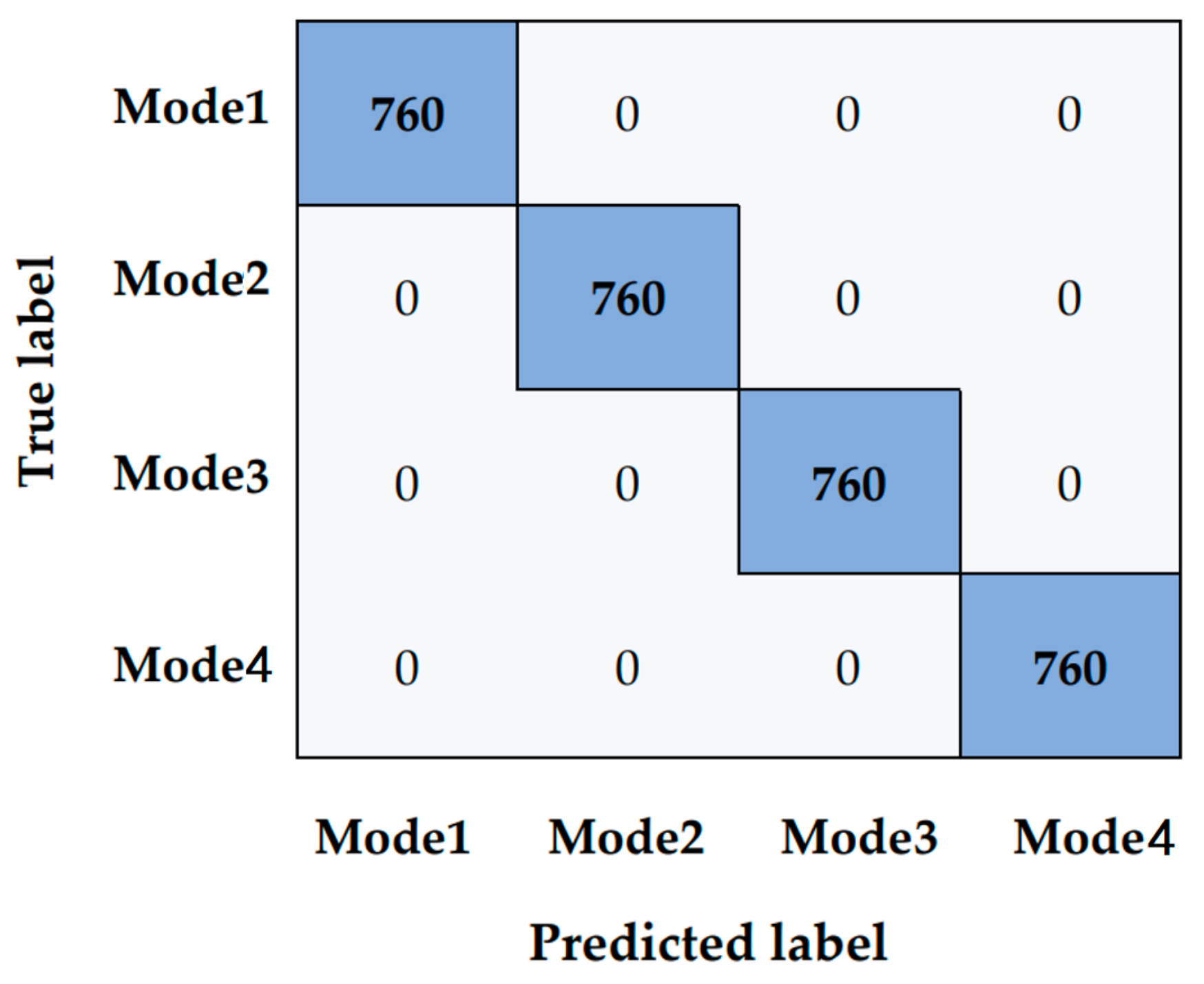
The confusion matrix of the toxic gas concentration interval detection task result is shown in Figure 8. We used a 10-fold validation method to test the results and set the number of verifications to 760. As shown in Figure 8, the accuracy rate was close to 100%. Mode 1 corresponded to the 0–10 ppm toxic gas interval, and Mode 4 corresponded to the 30–40 ppm toxic gas.
To compare toxic gas concentration interval detection accuracy and assess the method’s performance, we used two related methods. The comparative methods were convolutional neural networks (CNNs) + support vector machine (SVM) transformer encoder and ESS transformer. Table 1 lists the results for each of these methods. The CNN + SVM method had the lowest training time (480 s). Because of the transformer’s high parallel computing ability, the transformer encoder model had the highest training time (600 s). The proposed model had a higher recall score of 99% and a higher accuracy of 99.9%.

3.3.3. Health Levels and Lifetime Prediction Results and Discussion

As shown in Figure 9, the establishment of system health is closely related to prior knowledge of the sensor’s life. Therefore, we connected the four classification results for toxic gas concentration detection to the remaining lifetime of the CH4 sensor with toxic gas and broadcast the speech through the Ocean X GPT model.
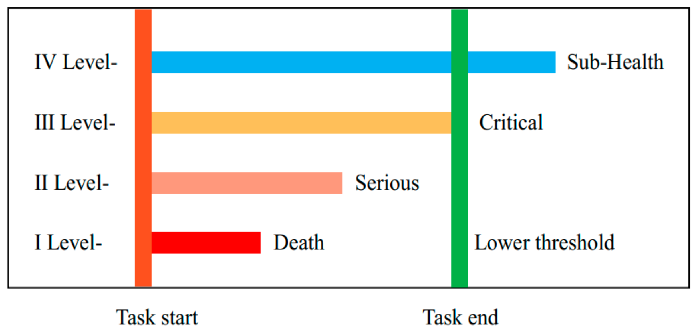
The mechanism of H2S poisoning of CH4 sensors is a complex chemical process. It is considered to be a chemical reaction between sensitive materials and sulfur and is specifically manifested as catalyst sulfur poisoning and sensitive material sulfur poisoning [10]. This poisoning affects the three most important indicators of activity, selectivity, and life of the CH4 sensors [11]. The phenomenon of CH4 sensor poisoning caused by H2S can be understood as the adsorption of poison at the surface’s active center and further conversion to more stable surface compounds. This action leads to the active site being passivated or permanently occupied. On the one hand, H2S gas makes the active component of the precious metal catalyst become inactive metal sulfide or sulfate. On the other hand, the sulfurization or sulfation of SnO2-sensitive materials makes it lose its role of supporting the active component and regulating the microstructure of the active component. The degree of CH4 sensor poisoning caused by H2S gas can be expressed by a grading system. The assessment is based on the remaining time that the sensor continues to work after the poisoning has occurred. According to the requirement of the one-time working time of the sensor for CH4 detection, we classified the H2S poisoning phenomenon into four grades. Figure 10 shows the H2S poisoning level of the CH4 sensor.
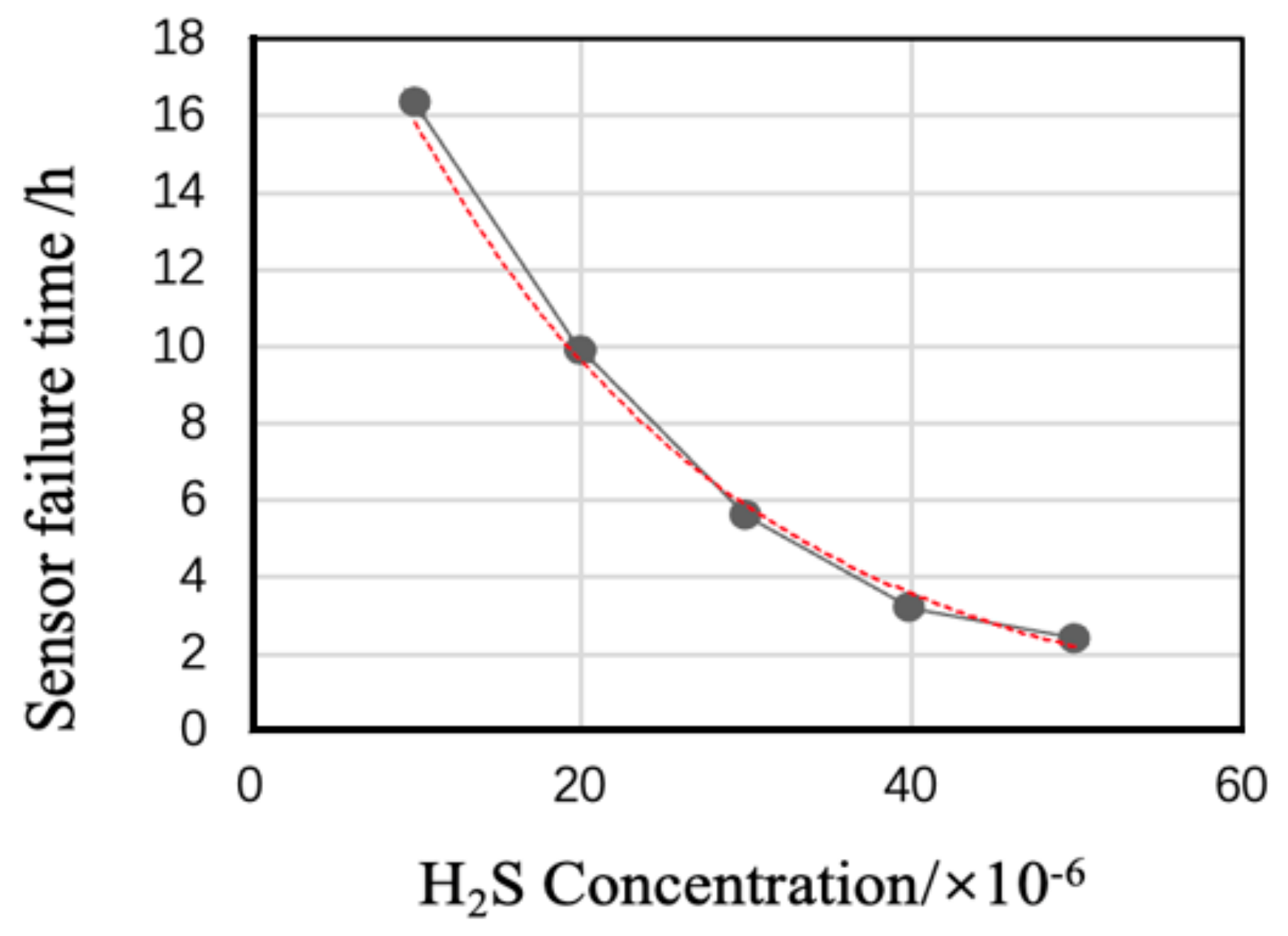
According to the general technical standards of gas sensors and specific engineering application requirements, we selected deviation from the CH4 detection value ±10% as the failure criterion of the CH4 sensor. After a qualified aging screening, we extracted and divided 10 MQ4 sensor samples (MQ4 and MQx6) into five groups for testing. We similarly assumed that the performance of the ten sensor arrays used for life calibration experiments to that of six sensor arrays in the toxic gas concentration internal detection experiment in real working conditions. We conducted the test under normal atmospheric conditions. To simulate real working conditions, we loaded environmental factors, such as vibration, rocking, and heating, into the test. We tested the failure time of H2S poisoning of the sensor in a fixed concentration interval according to relevant regulations. Figure 10 shows the relationship between H2S concentration and the failure time of the CH4 sensor. This figure can be used as a health management system reference to classify toxic gas concentration intervals.
As shown in Figure 10, the IV Level was the lowest level, in which case the detection would not be affected. The concentration of toxic gas (H2S) was 0–10 ppm. The III Level was the critical warning, which could cause the sensor detection accuracy to move to the edge of the error band and would not be able to maintain sensor detection accuracy within a specified time. The concentration of toxic gas (H2S) was 10–20 ppm. The II Level was higher, which caused the CH4 sensor to fail to complete the specified task within the specified time, but it could continue to work after recovery. The concentration of toxic gas (H2S) was 20–30 ppm. The I Level was the highest level, which caused fatal damage to the sensor, failed to complete the specified task within the specified time, and whose performance could not be restored. The concentration of toxic gas (H2S) was 30–40 ppm.
Therefore, according to Figure 9 and Figure 10, we obtained the following information about the health of the system:
The concentration of toxic gas internal detection at Mode 0 was 0–10 ppm, the health level was IV Level, and the remaining working time was about over 16 h.
The concentration of toxic gas internal detection at Mode 1 was 10–20 ppm, the health level was III Level, and the remaining working time was about 10–16 h.
The concentration of toxic gas internal detection at Mode 2 was 20–30 ppm, the health level was II Level, and the remaining working time was about 6–10 h.
The concentration of toxic gas internal detection at Mode 3 was 30–40 ppm, the health level was I Level, and the remaining working time was about 3–6 h.

3.3.4. Offline Question-and-Answer System Experimental Results and Discussion

We evaluated questions and answers from the CH4 sensor Wikipedia and model basics. These contents were the key factor affecting the working state of CH4 sensors. We trained the offline question-and-answer task for the health system for 500 iterations. Throughout this process, we set the batch size to two, and set the dynamic learning rate to 0.0001. As the number of training epochs rose, the learning rate dropped every 10 epochs by 0.0005. Therefore, the model was able to find the global optimum more quickly. Figure S5 shows the training and validation loss of the toxic gas concentration interval detection model.
Table 2 provides the accuracy of the offline question-and-answer system by Ocean X GPT. According to the results given in Table 2, the 12 questions were essentially correct, as they pertained to deep-sea CH4 detection (average accuracy was >99%). The question “What is the significance of predicting failure?” had the highest accuracy (99.9%), and the question “What is the mechanism of the sensor poisoning caused by H2S?” had the lowest accuracy (98.7%). These problems basically include all the knowledge points of sensor construction and abnormal fault detection. These questions can make the questioner learn the basic problems of engineering very well, which is of great help to the emergencies that occur in the actual working environment.
Figure S6 provides a visualization of the offline question-and-answer task by the Ocean X GPT model. It shows in detail the original corpus of the model, the trained questions, and the results of the trained answers. It can be seen that the model roughly correctly learns the key information in the original corpus and can accurately answer the questions without grammatical errors. This part combines the abnormal gas detection and the dialog system well, making the model have the concept of embodied intelligence. The model can simulate the real human feedback to the questioner through the external environment.
To compare the accuracy of the offline question-and-answer task and assess model performance, we selected two other models (Table 3). The comparative models were LSTM_Decoder and GPT Decoder (GPT Decoder). Ocean X GPT had the highest mean accuracy (99.4%), and LSTM_Decoder had the lowest accuracy. LSTM was not suitable as a model for discrete tasks. According to the number of tokens, the accuracy rate decreased by increasing the number of tokens, which was easy to understand. When the number of answering words increased, the required computing power increased, and it became more difficult to achieve the same accuracy rate.

3.4. Attention Visualization for Anomaly Detection in the Training Process

The training process included a thermodynamic diagram for the attention mechanism to detect the toxic gas concentration interval as well as an offline question-and-answer task (Figure 11). Figure 11a–d show the toxic gas concentration interval detection task, illustrating a thermodynamic diagram for the attention mechanism after training 50 epochs (MSE 0.07, MAE 0.06), 20 epochs (MSE 0.12, MAE 0.11), 10 epochs (MSE 0.38, MAE 0.32), and 5 epochs (MSE 0.68, MAE 0.41).
The Ocean X GPT task provided a thermodynamic diagram for the attention mechanism after training 500 epochs (CrossEntropy 0.02), 300 epochs (CrossEntropy 0.16), 100 epochs (CrossEntropy 0.84), and 50 epochs (CrossEntropy 1.39).

3.5. Comparison of Model Memory Cost

Table 4 compares similar efforts to limit time complexity. We employed three models for comparison, including Dai et al. (2019) [47], Child et al. (2019) [48], and Kitaev et al. (2020) [49]. The ESS transformer model limited the time complexity to O (nlogn) by using fixed patterns or combinations of fixed patterns. Model performance was not lost, and the effect was elegant.

4. Conclusions

In this study, we proposed two models for industrial conditions. We employed the ESS transformer model, which was used for toxic gas concentration interval detection under marine conditions. Furthermore, we employed the Ocean X GPT model, which embedded the ESS transformer model for intelligent health management and lifetime prediction of the CH4 sensor arrays. The ESS transformer model enhanced the performance of concentration interval detection under marine conditions (accuracy = 0.99). These results were superior to other similar models, including CNN + SVM and transformer encoder. The proposed model had a time complexity of only O (n logn) compared with the time complexity of the original model, which was O (n2). The ESS transformer model offered a beneficial solution for concentration interval detection under marine conditions. It offered high accuracy, high speed, and low computational complexity. The Ocean X GPT model for offline question-and-answer tasks had a high mean accuracy (99.4%), which was superior to other related models, such as LSTM–AE and GPT decoder. It also featured an elegant concept using a question-and-answer system framework.

Supplementary Materials

The following supporting information can be downloaded at: https://www.mdpi.com/article/10.3390/chemosensors12090172/s1, Figure S1: Implementation of rotary position embedding (RoPE); Figure S2: The transformer model for toxic gas concentration interval detection task and methane remote sensor arrays health management task: (a) Encoder; (b) Ocean X GPT; Figure S3: Correlation of toxic gas concentration interval detection data; Figure S4: Training and validation loss of toxic gas concentration interval detection model; Figure: S5: Training and validation loss of Ocean X GPT model; Figure S6: Visualization of offline question-answering task by Ocean X GPT model; Table S1: Parameters of toxic gas concentration interval detection model; Table S2: Parameters of Ocean X GPT model [45,46,50,51,52].

Author Contributions

Conceptualization, K.Z., Y.Z. and J.W.; formal analysis, T.W.; methodology, W.J.; writing—original draft preparation, K.Z.; writing—review and editing, M.Z. and Z.Y.; funding acquisition, M.Z. and Z.Y. All authors have read and agreed to the published version of the manuscript.

Funding

This work was supported by the National Key Research and Development Program of China (2022YFC3104700), the National Natural Science Foundation of China (62371299, and 62301314), and the China Postdoctoral Science Foundation (2023M732198). We also acknowledge analysis support from the Instrumental Analysis Center of Shanghai Jiao Tong University and the Center for Advanced Electronic Materials and Devices of Shanghai Jiao Tong University. The computations in this paper were run on the π 2.0 cluster supported by the Center for High Performance Computing at Shanghai Jiao Tong University.

Institutional Review Board Statement

Not applicable.

Informed Consent Statement

All the participants signed the informed consent and the related information sheet, in which the study was explained, before participating in the experiment.

Data Availability Statement

For privacy reasons, given the sensitive nature of the data, the aggregated data analyzed in this study will not be publicly disclosed but might be available on request from the corresponding author.

Conflicts of Interest

The authors declare no conflicts of interest. The funders had no role in the design of the study; in the collection, analyses, or interpretation of data; in the writing of the manuscript; or in the decision to publish the results.

References

  1. Liu, M.; Xue, M.; Cui, X.; Peng, W. A review on the methane emission detection during offshore natural gas hydrate production. Front. Energy Res. 2023, 11, 12607–12617. [Google Scholar]
  2. Ying, W.; Xu, G.; Hong, Z. Characteristics and emissions of isoprene and other non-methane hydrocarbons in the Northwest Pacific Ocean and responses to atmospheric aerosol deposition. Sci. Total Environ. 2023, 10, 162808. [Google Scholar]
  3. Irina, T.; Ilya, F.; Aleksandr, S. Mapping onshore CH4 seeps in Western Siberian floodplains using convolutional neural network. Remote Sens. 2022, 14, 2611. [Google Scholar]
  4. Itziar, I.; Javier, G.; Daniel, Z. Satellites detect a methane ultra-emission event from an Offshore Platform in the Gulf of Mexico. Environ. Sci. Technol. Lett. 2022, 9, 520–525. [Google Scholar]
  5. Ian, B.; Vassilis, K.; Andrew, R. Simultaneous high-precision, high-frequency measurements of methane and nitrous oxide in surface seawater by cavity ring-down spectroscopy. Front. Mar. Sci. 2023, 10, 186–195. [Google Scholar]
  6. Xuan, Z.; Miaomiao, Z.; Lingbing, B. Simulation and error analysis of methane detection globally using spaceborne IPDA Lidar. Remote Sens. 2023, 15, 3239. [Google Scholar]
  7. Wei, K.; Thor, S. A review of gas hydrate nucleation theories and growth models. J. Nat. Gas Sci. Eng. 2019, 61, 169–196. [Google Scholar]
  8. Abrahamsson, K.; Damm, E.; Björk, G.; Bunse, C.; Sellmaier, S.; Broström, G.; Assmann, V.; Dumitrascu, A.; Maciute, A.; Olofsson, N.; et al. Methane plume detection after the 2022 Nord stream pipeline explosion in the Baltic Sea. Nature 2024, 14, 12848. [Google Scholar] [CrossRef]
  9. Cooper, L.J.; Dubey, A. Hawkes, Methane detection and quantification in the upstream oil and gas sector: The role of satellites in emissions detection, reconciling and reporting. Environ. Sci. Atmos. 2022, 2, 9–23. [Google Scholar] [CrossRef]
  10. Xi-lai, L.; Meng-han, W.; Yong, H. Influences of Impurity Gases in Air on Room-Temperature Hydrogen-Sensitive Pt–SnO2 Composite Nanoceramics: A Case Study of H2S. Chemosensors 2023, 11, 31. [Google Scholar] [CrossRef]
  11. Yuan, Z.; Yang, C.; Meng, F. Strategies for improving the sensing performance of semiconductor gas sensors for high-performance formaldehyde detection: A review. Chemosensors 2021, 9, 179. [Google Scholar] [CrossRef]
  12. Chen, Y.S.; Xu, Y.H. Fault detection, isolation, and diagnosis of status self-validating gas sensor arrays. Rev. Sci. Instrum. 2010, 87, 045001. [Google Scholar] [CrossRef]
  13. Sana, J.; Young, L.; Jungpil, S. Sensor fault classification based on support vector machine and statistical time-domain features. IEEE Access 2017, 5, 8682–8690. [Google Scholar]
  14. Yang, J.; Chen, Y. An efficient approach for fault detection, isolation, and data recovery of self-validating multifunctional sensors. IEEE Trans. Instrum. Meas. 2017, 66, 543–558. [Google Scholar] [CrossRef]
  15. Gao, Z.; Cecati, C.; Ding, S.X. A survey of fault diagnosis and fault tolerant techniques—Part I: Fault diagnosis with model-based and signal-based approaches. IEEE Trans. Ind. Electron. 2015, 62, 3757–3767. [Google Scholar]
  16. Lu, J.; Huang, J.; Lu, F. Sensor fault diagnosis for aero engine based on online sequential extreme learning machine with memory principle. Energies 2017, 10, 39. [Google Scholar] [CrossRef]
  17. Tsui, K.L.; Chen, N. Prognostics and health management: A review on data driven approaches. Math. Probl. Eng. 2015, 6, 793161. [Google Scholar] [CrossRef]
  18. Bai, G.; Wang, P.; Hu, C. A self-cognizant dynamic system approach for prognostics and health management. J. Power Sources 2015, 278, 163–174. [Google Scholar] [CrossRef]
  19. Coble, J.; Ramuhalli, P.; Bond, L. A review of prognostics and health management applications in nuclear power plants. Int. J. Progn. Health Manag. 2015, 6, 1–22. [Google Scholar]
  20. Shen, Z.; He, Z. A monotonic degradation assessment index of rolling bearings using fuzzy support vector data description and running time. Sensors 2012, 12, 10109–10135. [Google Scholar] [CrossRef]
  21. Sohaib, M.; Kim, C.H.A. Hybrid feature model and deep-learning-based bearing fault diagnosis. Sensors 2017, 17, 2876. [Google Scholar] [CrossRef] [PubMed]
  22. Wang, J.; Wang, X.; Wang, L. Modeling of BN lifetime prediction of a system based on integrated multi-level information. Sensors 2017, 17, 2123. [Google Scholar] [CrossRef] [PubMed]
  23. Agarwal, V.; Lybeck, N.J. Development of Asset Fault Signatures for Prognostic and Health Management in the Nuclear Industry; Prognostics and Health Management: Austin, TX, USA, 2015; pp. 1–7. [Google Scholar]
  24. Kumar, S.; Pecht, M. Modeling approaches for prognostics and health management of electronics. Int. J. Perform. Eng. 2010, 6, 222–229. [Google Scholar]
  25. Feng, Z.G.; Wang, Q. Research on health evaluation system of liquid-propellant rocket engine ground-testing bed based on fuzzy theory. Acta Astronaut. 2007, 61, 840–853. [Google Scholar] [CrossRef]
  26. Xia, T.; Xi, L. Dynamic maintenance decision-making for series–parallel manufacturing system based on MAM–MTW methodology. Eur. J. Oper. Res. 2012, 221, 231–240. [Google Scholar] [CrossRef]
  27. Berges, L.; Galar Gustafson, A. Maintenance decision making based on different types of data fusion. Eksploat. I Niezawodn.-Maint. Reliab. 2012, 14, 135–144. [Google Scholar]
  28. Cates, G.L.; Skinner, C.H.; Watson, T.S. Instructional effectiveness and instructional efficiency as considerations for data-based decision making: An evaluation of interspersing procedures. Sch. Psychol. Rev. 2003, 32, 601–616. [Google Scholar] [CrossRef]
  29. Chen, Y.; Jiang, S.; Yang, J. Grey bootstrap method for data validation and dynamic uncertainty estimation of self-validating multifunctional sensors. Chemometr. Intell. Lab. Syst. 2015, 146, 63–76. [Google Scholar] [CrossRef]
  30. Song, K.; Wang, Q. In quantitative measurement of gas component using multi-sensor array and NPSO-based LS-SVR. Instrum. Meas. Technol. Conf. 2013, 80, 1740–1743. [Google Scholar]
  31. Shen, Z.; Wang, Q. Data-driven health evaluation of multifunctional self-validating sensor using health reliability degree. Inf. Technol. J. 2012, 11, 1597–1604. [Google Scholar] [CrossRef]
  32. Shen, Z.; Wang, Q. A novel health evaluation strategy for multifunctional self-validating sensors. Sensors 2013, 13, 587–610. [Google Scholar] [CrossRef] [PubMed]
  33. Aughenbaugh, J.M.; Herrmann, J.W. Reliability-based decision making: A comparison of statistical approaches. J. Stat. Theory Pract. 2009, 3, 289–303. [Google Scholar] [CrossRef]
  34. Wang, A.; Jiang, J.; Zhang, H. Multi-sensor image decision level fusion detection algorithm based on D-S evidence theory. In Proceedings of the Fourth International Conference on Instrumentation and Measurement, Computer, Communication and Control, Harbin, China, 18–20 September 2014; pp. 620–623. [Google Scholar]
  35. He, Z.; Zhang, H.; Zhao, J. Classification of power quality disturbances using quantum neural network and DS evidence fusion. Eur. Trans. Electr. Power 2013, 22, 533–547. [Google Scholar] [CrossRef]
  36. Wang, H.; Lin, D. Research on multi-objective group decision-making in condition-based maintenance for transmission and transformation equipment based on D-S evidence theory. IEEE Trans. Smart Grid 2015, 6, 1035–1045. [Google Scholar] [CrossRef]
  37. Lin, S.; Li, C. The strategy research on electrical equipment condition-based maintenance based on cloud model and grey D-S evidence theory. Intell. Decis. Technol. 2018, 3, 283–292. [Google Scholar] [CrossRef]
  38. Mehta, P.; Werner, A. Condition based maintenance-systems integration and intelligence using Bayesian classification and sensor fusion. J. Intell. Manuf. 2015, 26, 331–346. [Google Scholar] [CrossRef]
  39. Herrle, S.R.; Corbett, E.C. Bayes’ theorem and the physical examination: Probability assessment and diagnostic decision making. Acad. Med. J. Assoc. Am. Med. Coll. 2011, 86, 618. [Google Scholar] [CrossRef]
  40. Lin, P.C.; Gu, J.C.; Yang, M.T. Intelligent maintenance model for condition assessment of circuit breakers using fuzzy set theory and evidential reasoning. IET Gener. Transm. Distrib. 2014, 8, 1244–1253. [Google Scholar] [CrossRef]
  41. Yin, K.; Yang, B.; Li, X. Multiple attribute group decision-making methods based on trapezoidal fuzzy two-dimensional linguistic partitioned bonferroni mean aggregation operators. Int. J. Environ. Res. Public Health 2018, 15, 194. [Google Scholar] [CrossRef]
  42. Chen, S.; Cheng, S.; Chiou, C. Fuzzy multi-attribute group decision making based on intuitionistic fuzzy sets and evidential reasoning methodology. Inf. Fusion 2016, 27, 215–227. [Google Scholar] [CrossRef]
  43. Efe, B. An integrated fuzzy multi criteria group decision making approach for ERP system selection. Appl. Soft Comput. 2016, 38, 106–117. [Google Scholar] [CrossRef]
  44. Joshi, D.; Kumar, S. Interval-valued intuitionistic hesitant fuzzy Choquet integral based TOPSIS method for multi-criteria group decision making. Eur. J. Oper. Res. 2016, 248, 183–191. [Google Scholar] [CrossRef]
  45. Zhou, H.; Zhang, S.; Peng, J.; Zhang, S.; Li, J.; Xiong, H.; Zhang, W. Informer: Beyond efficient transformer for long sequence time-series forecasting. Proc. AAAI Conf. Artif. Intell. 2021, 35, 12. [Google Scholar] [CrossRef]
  46. Su, J.; Ahmed, M.; Lu, Y.; Pan, S.; Bo, W.; Liu, Y. RoFormer: Enhanced transformer with Rotary Position Embedding. Neurocomputing 2024, 568, 127063. [Google Scholar] [CrossRef]
  47. Dai, Z.; Yang, Z.; Yang, Y.; Carbonell, J.; Le, Q.V.; Salakhutdinov, R. Transformer-XL: Attentive language models beyond a fixed-length context. arXiv 2019, arXiv:1901.02860. [Google Scholar]
  48. Child, R.; Gray, S.; Radford, A.; Sutskever, I. Generating long sequences with sparse transformers. arXiv 2019, arXiv:1904.10509. [Google Scholar]
  49. Kitaev, N.; Kaiser, Ł.; Levskaya, A. Reformer: The efficient transformer. Int. Conf. Learn. Represent. 2020, 4, 148–156. [Google Scholar]
  50. Vaswani, A.; Shazeer, N. Attention is all you need. Adv. Neural Inf. Process. Syst. 2017, 4–9, 5998–6008. [Google Scholar]
  51. Katharopoulos, A.; Vyas, A.; Pappas, N.; Fleuret, F. Transformers are RNNs: Fast autoregressive transformers with linear attention. Int. Conf. Mach. Learn. 2020, 119, 5156–5165. [Google Scholar]
  52. Shen, Z.; Zhang, M. Efficient Attention: Attention with Linear Complexities. WACV 2021, 8, 3530–3538. [Google Scholar]
Figure 1. (a) Factorized transformer (fixed), (b) factorized transformer (strided), (c) transformer (decoder mask), and (d) ESS mask.
Chemosensors 12 00172 g001
Figure 2. Query and key matrix multiplication weight sorting results.
Chemosensors 12 00172 g002
Figure 3. (a) Self-attention module and (b) ESS attention module.
Chemosensors 12 00172 g003
Figure 4. (a) Self-attention module and (b) enhanced-RoPE module.
Chemosensors 12 00172 g004
Figure 5. Experimental setups using the gas sensor arrays: (a) experimental system diagram, (b) gas sensor circuit diagram, and (c) MQ4 and MQx6 CH4 gas sensors and internal functional components of sensors.
Chemosensors 12 00172 g005
Figure 6. Different kinds of toxic gas concentration intervals: (a) signal of 0–10 ppm toxic gas; (b) signal of 10–20 ppm toxic gas; (c) signal of 20–30 ppm toxic gas; (d) signal of 30–40 ppm toxic gas; and (e) signal of different combinations of toxic gas (H2S) concentration interval.
Chemosensors 12 00172 g006
Figure 7. Experimental flow charts of the proposed method.
Chemosensors 12 00172 g007
Figure 8. Toxic gas concentration interval detection results from the ESS transformer model. Confusion matrix of classification task result.
Chemosensors 12 00172 g008
Figure 9. Relationship between failure time and H2S concentration.
Chemosensors 12 00172 g009
Figure 10. Severity classification of H2S poisoning by CH4 sensor.
Chemosensors 12 00172 g010
Figure 11. Attention visualization for training data of toxic gas concentration interval detection task and offline question-and-answer task: (a) Epoch 5, MSE 0.68, MAE 0.41; (b) Epoch 10, MSE 0.38, MAE 0.32; (c) Epoch 20, MSE 0.12, MAE 0.11; (d) Epoch 50, MSE 0.07, MAE 0.06, (e) Epoch 50, CrossEntropy 1.39; (f) Epoch 100, CrossEntropy 0.84; (g) Epoch 300, CrossEntropy 0.16; and (h) Epoch 500, CrossEntropy 0.02.
Chemosensors 12 00172 g011
Table 1. Toxic gas concentration detection metrics for the three methods.
ModelTraining Time
(s)
Accuracy
(%)
Recall
(%)
Testing Time
(s)
CNN + SVM48097.5%97%0.1
Transformerencoder60098.3%98%0.2
ESS transformer model52099.9%99%0.2
Table 2. Offline question-and-answer accuracy by Ocean X GPT.
QuestionGenerated Answer TokenCorrectAccuracy Rate
(%)
What are the application areas of CH4 sensors?3799.7%
What are the H2S poisoning phenomena of sensors?4099.4%
What are the hazards of CH4 gas?3999.9%
What is the transformer algorithm?4699.5%
What are the implications of detecting ocean CH4?3799.2%
What are the components of an array sensor?4099.6%
What are the components of the signal collector?
What are the gas identification methods?
41
56

99.3%
98.9%
What is the mechanism of sensor poisoning caused by H2S?5298.7%
What is the degree of poisoning of the CH4 sensor arrays caused by H2S gas?8498.9%
What is the level of H2S?5299.1%
What is the significance of predicting failure?1599.9%
Table 3. Accuracy of offline question-and-answer tasks using three models.
ModelMean
Accuracy
<40
Tokens
40–50
Tokens
>50
Tokens
Prompt
or Not
I Do Not Know Assignment
LSTM-ecoder96.6%97.1%96.5%96.2%No
GPTDecoder98.1%98.3%98.1%97.9%No
Ocean X GPT99.4%99.7%99.5%98.9%No
Table 4. ESS transformer model summary.
Model/PaperComplexityDecodeClass
Trans.-XL (Dai et al., 2019) [47]O(n2) RC
Sparse Trans. (Child et al., 2019) [48] O ( n n ) FP
Reformer (Kitaev et al., 2020) [49]O(nlogn) LP
ESS transformer modelO(nlogn) X FP
Ps: Class abbreviations include FP = Fixed Patterns or Combinations of Fixed Patterns, LP = Learnable Pattern, RC = Recurrence.
Disclaimer/Publisher’s Note: The statements, opinions and data contained in all publications are solely those of the individual author(s) and contributor(s) and not of MDPI and/or the editor(s). MDPI and/or the editor(s) disclaim responsibility for any injury to people or property resulting from any ideas, methods, instructions or products referred to in the content.