1. Introduction
Potato is one of the most important food crops worldwide, ranking just behind rice, wheat, and maize in terms of production volume [
1,
2]. However, potatoes are highly susceptible to microbial invasions, including bacteria and fungi, during storage and transportation, which can lead to rot [
3]. This decay not only affects the quality and market value of the product but also leads to significant economic losses for farmers and other stakeholders throughout the supply chain [
4]. Therefore, effectively detecting and assessing the degree of potato rot, especially distinguishing between different levels of decay, has become a pressing issue that needs to be addressed. In recent years, with the increasing demand for food quality assessment, the automated detection of rot levels has gradually become a research focus with significant practical importance [
5,
6].
Current methods for automatic potato rot detection mainly include computer vision technology, spectroscopic analysis, and electronic nose (e-nose) detection based on odor sensors. Computer vision technology primarily relies on detecting surface visual changes, which limits its ability to identify rot that occurs internally [
7,
8,
9,
10]. Spectroscopic analysis, which can capture the chemical composition and internal structure of samples, improves detection depth to some extent but remains limited in detecting stacked potatoes and requires complex equipment with stringent operating conditions [
11,
12]. In contrast, the e-nose, which mimics the human sense of smell by capturing volatile compounds released during decay, has shown significant potential for potato rot detection. Loulier et al. used an e-nose combined with an SPME-GC/MS platform to detect fungi and oomycetes, and they demonstrated the effectiveness of the e-nose in distinguishing these microorganisms [
13]. Similarly, Biondi et al. showed that the e-nose could effectively detect potato brown rot and ring rot in both laboratory and large-scale applications [
14]. However, current e-nose signal analysis methods primarily rely on linear dimensionality reduction techniques, such as Principal Component Analysis (PCA), or simple statistical analysis, which are insufficient for handling the high-dimensional and nonlinear characteristics of multi-sensor signals [
15,
16,
17].
To address the shortcomings of e-nose signal analysis, some researchers have introduced machine learning techniques for e-nose data processing [
18,
19,
20]. Rutolo et al. applied PCA and Support Vector Machine (SVM) approaches to successfully use e-nose technology for the early detection of soft rot in potatoes, achieving promising results [
21]. Although machine learning methods have improved the processing and analysis of e-nose signals to some extent, they are still highly dependent on the quality and quantity of data, making manual feature extraction complex and incapable of capturing high-order and nonlinear features present in e-nose signals [
3,
22]. In practical applications, highly decayed potatoes are more susceptible to microbial infection, which results in complex changes in the concentration of volatile compounds, such as aldehydes, alcohols, and ketones, thus affecting the response strength of e-nose signals. With traditional machine learning methods, it is challenging for models to accurately differentiate such complex signal characteristics, especially when it comes to distinguishing different rot levels. Therefore, a more accurate assessment of rot severity, beyond just identifying decayed potatoes, is essential.
In recent years, deep learning methods have demonstrated superior performance in automatic feature extraction and complex signal processing [
23,
24,
25,
26]. Lin et al. combined Convolutional Neural Networks (CNNs) to analyze potato rot, showing the potential of deep learning in feature extraction and rot-level prediction [
27]. However, deep learning methods are also prone to overfitting when data samples are insufficient, particularly in complex multi-level rot classification tasks. To alleviate the data scarcity problem and improve the generalization performance of deep learning models, data augmentation techniques have been widely applied, among which Generative Adversarial Networks (GANs) are among the most commonly used due to their superior performance in data generation [
28]. However, directly applying traditional GANs to e-nose signal generation may lead to challenges in maintaining class separability, especially given the complex components and high-dimensional features of e-nose data, where the class boundaries among different rot levels may not be clearly preserved [
29]. Therefore, improved generative methods are needed to better adapt to the characteristics of e-nose signals and enhance the class separability of the generated data.
To address the challenges of fine-level rot detection under environmental interference during potato storage, as well as the problem of data scarcity, this study proposes the following solutions: (1) to design a Gaussian Mixture Embedded Generative Adversarial Network (GMEGAN), which integrates a Variational Autoencoder (VAE), Gaussian Mixture Model (GMM), and GAN to overcome the scarcity of multi-level rot samples and enhance the diversity and class separability of the generated data; (2) to propose a method that combines Conditional Convolutional Neural Networks (Conditional CNNs) with feature-optimized channel attention modules (f-CAM, f-ECA) to improve the feature extraction and prediction accuracy of rot-level classification models; (3) to conduct data augmentation experiments to verify the effectiveness of the generated data and evaluate the impact of the augmented datasets on different machine learning and deep learning classification models, significantly improving the accuracy and robustness of rot-level detection.
2. Materials and Methods
2.1. Sample Preparation
The experimental samples comprised 500 kg of Zhongshu No. 5 potatoes, obtained from the Agricultural Science Institute of Jinhua, Zhejiang Province, China. The potatoes were initially stored in a cool, dark environment at approximately 15 °C for two weeks to allow surface drying and the healing of wounds. Subsequently, diseased potatoes were manually removed, and the remaining potatoes were treated with a chlorpropham sprout suppressant for 48 h. After treatment, all potatoes were then stored in a ventilated chamber at 4–8 °C with approximately 90% relative humidity for four months. Based on the degree of rot, the samples were categorized into three groups: normal, slightly rotten, and severely rotten. Slight rot was characterized by darkened skin, softened tissues, spots, and a slight off-odor; severe rot was characterized by skin damage, white fungal plaques, internal tissue turning into a cotton-like or viscous liquid, and a strong offensive odor.
According to the GB/T 31784-2015 “Classification and Inspection Procedure for Commodity Potatoes” standard, approximately 10 kg of potatoes was randomly selected for test samples, which were further categorized into normal, slightly rotten, and severely rotten, with 120 samples in each category. Specifically, based on the rotting ratio standards for table potatoes (not exceeding 0.5%, 3%, and 5%), we selected the ranges of 0–0.5%, 0.5–3%, and 3–5% to prepare slightly rotten samples with the corresponding weights of rotten potatoes within each sample being 0–50 g, 50–300 g, and 300–500 g, respectively. For each rot degree, 40 samples were prepared for each rotting ratio, resulting in a total of 120 samples for each rot category The normal samples were periodically obtained by selecting 10 healthy potatoes from storage every 12 days for a total of 120 samples. Finally, the total of 360 samples were split into a training set and a testing set .
2.2. Electronic Nose Detection System
The electronic nose detection system self-developed in our lab comprises four main components: the electronic nose device, client terminal, MQTT server, and environmental monitoring module [
27], all of which are deployed within the same local area network (LAN) and communicate via Wi-Fi (
Figure 1). The electronic nose device consists of a control module, sampling circuit, gas chamber, gas path, power supply module, and wireless communication module. It is responsible for collecting sample data, which is aggregated at the end of each 180 s cycle (12 × 180 resistance values), and transmitted in real time to the client via the MQTT server. The client is developed using the Qt platform with capabilities for data management and interaction with a MySQL database as well as supporting experiment parameter settings, signal visualization, and the deployment of custom-designed neural network models for online detection.
The gas chromatography-ion mobility spectrometry (GC-IMS) analysis, as shown in
Figure 2, revealed the volatile compounds emitted from rotten potatoes, which include 4 aldehydes, 9 ketones, 12 alcohols, 6 esters, 6 alkenes, 2 furans, 2 aromatic hydrocarbons, and 1 sulfide compound [
27]. Representative compounds include glyoxal, heptanal, styrene, isobutanol, and furan, which have also been reported in other studies [
3]. These compounds were selected as the primary target gases for detection, as they are key indicators of potato decay and have been shown to correlate with different stages of spoilage. To detect these volatile markers, 12 metal oxide semiconductor (MOS) sensors were selected to form the electronic nose sensor array with details of each sensor’s characteristics listed in
Table 1 [
27]. These sensors were chosen for their ability to detect a wide range of volatile compounds, including those identified by GC-IMS, with the added advantage of providing real-time responses. The selection of the MOS sensor array allows for the comprehensive detection of the gases emitted during potato decay and ensures robust measurement even in the presence of non-target gases.
The experiments were conducted in a cold storage environment, and the relevant experimental parameters are provided in
Table 2. These parameters were adapted from our previous study [
27] to suit the current experimental setup.
During the experiments, the electronic nose was used to detect headspace gases from normal, slightly rotten, and severely rotten potatoes. Each sample produced 12 × 180 response signals, where each value corresponds to the normalized sensor output. The response signal is derived using the relative difference method, comparing the sensor’s conductivity in the target gas (G) to its conductivity in clean air (G0), compensating for baseline drift and sensor aging effects. The detection procedure was as follows: (1) the sample container was allowed to sit for 10 min to generate headspace gases; (2) polytetrafluoroethylene (PTFE) tubes were used to connect the sample container to the electronic nose, allowing the pump to circulate the headspace gases into the gas chamber; (3) clean air filtered by activated carbon was injected into the gas chamber for 60 s to initialize the sensors to the baseline and stabilize the chamber temperature; (4) headspace gases were introduced into the gas chamber, and the response signal was recorded for 90 s, during which most signals reached a stable state; (5) the sensor array was flushed with clean air for 90 s to bring the sensor signals back to baseline.
2.3. Feature-Optimized Channel Attention Conditional Convolutional Neural Network
With the growing application of deep learning, Convolutional Neural Networks (CNNs) have demonstrated excellent performance in the field of electronic nose pattern recognition. For multi-channel time-series data, recent studies have introduced channel attention modules to learn correlations between different channels. These modules enable the neural network to automatically evaluate the significance of each channel, allocate optimal weights, and thereby focus on crucial channel features while reducing interference from correlated channels.
2.3.1. Feature-Optimized Channel Attention Module
Efficient Channel Attention (ECA) and Convolutional Block Attention Module (CBAM) are commonly used channel attention modules [
30]. The ECA module applies global average pooling to compress data from each channel into a single value. It introduces a non-dimensional reduction strategy, using a 1 × 1 convolution kernel to learn inter-channel importance and output channel weights. The channel attention part of CBAM (CAM) extends the Squeeze-and-Excitation (SE) [
31] module by adding global max pooling and then applying fully connected layers of the same length as the input and output to produce two sets of channel weights, which are added together and activated via a sigmoid function to obtain the final channel weights.
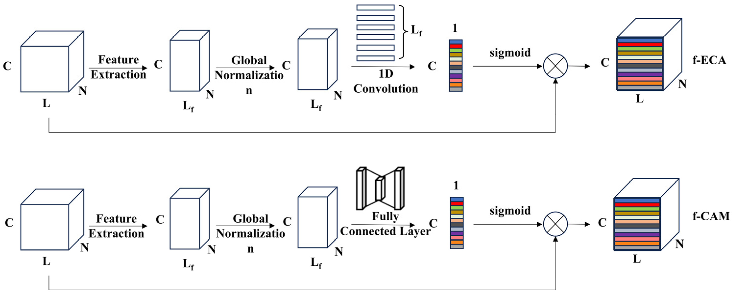
These modules are primarily used for extracting features from complex data by applying global or max pooling to each channel, resulting in a single value that represents channel-specific information. However, in the case of electronic nose data, each channel represents a one-dimensional time series, and using global pooling can result in significant information loss. Therefore, this study employs feature extraction methods to capture channel-specific characteristics, thereby optimizing the structure of the channel attention module, as shown in
Figure 3. Instead of using average pooling or max pooling, feature extraction was used to better capture the channel features of electronic nose data. Since SE modules compress inter-channel information and may lose some features, limiting the ability to fully capture dependencies between channels, the ECA and CAM modules were optimized in this study. Features were extracted from the original channel responses of the electronic nose, resulting in N features. Two feature-optimized channel attention modules, f-CAM and f-ECA, were developed using different neural network structures. As show in
Figure 3, N represents the total number of samples, L represents the signal length, C represents the number of channels, and L
f represents the number of features. f-CAM uses fully connected layers to compress and decompress channel features, while f-ECA employs one-dimensional convolution to selectively connect across channels.
2.3.2. Model Structure
To mitigate the interference caused by the mixture of potatoes with varying degrees of rot, a Conditional Convolutional Neural Network (Conditional CNN) was designed, which integrates the feature-optimized channel attention modules. The overall model structure is depicted in
Figure 4.
To determine the optimal hyperparameters for the convolutional layers, the convolution kernel size was varied within the range of [3, 5], while the number of kernels was selected from [64, 128, 256], resulting in a total of 216 model combinations. Each model was trained for 100 epochs on the training set
, and classification accuracy on the test set
was used to evaluate performance. Grid search was employed to find the best parameter combination. The 1D-CNN model parameters are detailed in
Table 3. Categorical cross-entropy was used as the loss function for gradient descent.
Based on the original CNN, the Conditional CNN adds a rot level vector as an input between the convolutional layers and the fully connected layer. The convolutional layers extract features from the electronic nose data, and these are then expanded into a [N, 640] two-dimensional vector and concatenated with the rot level vector before being fed into the fully connected layer. This allows the fully connected layer to take into account the varying degrees of rot when mapping features to categories. This approach enables the model to more effectively fit conditional probabilities, thereby reducing the impact of mixed rot levels on the classification of potato rot grades.
2.4. Gaussian Mixture Embedding Generative Adversarial Network (GMEGAN)
Due to the significant time and effort required to collect large amounts of electronic nose data, traditional machine learning methods, which require relatively small datasets, have been widely used in electronic nose pattern recognition. However, with advances in deep learning, its automated feature extraction and superior data-fitting capabilities have frequently surpassed traditional methods in analyzing electronic nose data.
The response signals from electronic noses applied to potatoes are closely associated with their rot levels, and the data distributions for samples across different rot levels show significant variation. To learn the deep latent features from these response signals and associate them with potato rot levels, we propose a Gaussian Mixture Embedding Generative Adversarial Network (GMEGAN). This model combines a Variational Autoencoder (VAE) [
32,
33,
34], a Gaussian Mixture Model (GMM) [
35], and a Conditional Generative Adversarial Network (GAN) [
28] to generate synthetic data that corresponds to different rot levels.
2.4.1. GMEGAN Architecture and Components
GMEGAN integrates VAE, GMM, and GAN to extract the latent features from electronic nose data and generate high-quality synthetic data. The model structure is shown in
Figure 5. The model consists of five components: the Encoder (
E), Gaussian Mixture Model (GMM), Generator (
G), Discriminator (
D), and Auxiliary Classifier (
C). The Encoder comprises three one-dimensional convolutional layers followed by two fully connected layers, which eventually output two separate fully connected layers to generate the mean and logarithmic standard deviation of the latent features. The GMM includes three Gaussian components along with their respective weights to capture the latent feature distributions of different sample categories. The Generator is composed of fully connected layers, with an input dimension of the latent feature space (40), while the Discriminator consists of three fully connected layers. The Auxiliary Classifier is a simple pre-trained classifier composed of three fully connected layers, which evaluates the validity of the generated data.
The GMEGAN framework merges the VAE’s capability to extract low-dimensional latent representations with the GMM’s adaptability to model complex data distributions. By incorporating GANs, GMEGAN enhances the decoder’s generative capability, producing diverse, high-quality synthetic data. These synthetic data maintain statistical similarity with the original dataset and preserve feature differences across samples with different rot levels.
2.4.2. Inference and Generation Process
The GMEGAN model uses the Encoder (E) and Generator (G) to model latent features and data, as illustrated in
Figure 6.
In the inference process, according to Bayes’ theorem, the posterior probability can be decomposed into two parts, one of which is approximated by a Gaussian Mixture Model. To reduce errors caused by inaccurate category inference during the GMM training process, supervised information is introduced during training to guide the GMM. When a sample
is given, the category
is known and independent of the latent variable
, leading to the following equations:
To ensure category accuracy during the generation process, especially when there is significant overlap between Gaussian components of different categories, directly mapping from the latent space to the data space may introduce incorrect category information. Therefore, it is necessary to include a category signal during the generation process to guide the Generator’s sampling, as shown in Equation (3):
2.4.3. Loss Function
The loss function of the GMEGAN model comprises several components: reconstruction loss, KL loss, GAN loss, cross-entropy loss, conditional loss, and Gaussian mixture loss.
Reconstruction loss:
The reconstruction loss measures the difference between generated data and original data, as shown in Equation (4):
where
is the number of Monte Carlo samples,
and
represent the
-th dimension of the
-th real data and reconstructed data, respectively, and Discriminator (D) is the data length.
KL loss;
The KL loss measures the similarity between the latent distribution generated by the encoder and the Gaussian Mixture Model, as shown in Equation (5):
where
and
are the mean and standard deviation of the
-th dimension of the sample
, and
and
are the mean and standard deviation of the
-th dimension of the
-th Gaussian component. It can be seen that
is only related to the category distribution of
, so the Lagrange multiplier method is used for optimization, as shown in Equation (6). The final
expression is shown in Equation (7), where
represents the amount of training set data.
Cross-entropy loss:
The cross-entropy loss ensures that the generated data have correct category characteristics, as shown in Equation (10):
where
is the number of generated samples from the Gaussian mixture distribution, and
is the output of the
for sample
Conditional loss:
The conditional loss ensures that the generated data conform to specific category conditions, as shown in Equation (11):
where
is the weight of the
-th fully connected layer of the Auxiliary Classifier
, and
represents the corresponding weight dimension.
Combining all the above loss components, the final loss function of the GMEGAN model is given by Equation (12):
2.4.4. Training Strategy
To train the Gaussian Mixture Embedding Generative Adversarial Network (GMEGAN), the following steps are taken to pre-train and optimize different components of the model.
Input the training dataset into encoder
, which outputs feature encoding
via
. The Generator
decodes
to generate data
. The Encoder (E) and Generator
are pre-trained using stochastic gradient descent with the loss function given as shown in Equation (13):
Input the training data into Encoder
to obtain the feature encoding, and use the mean and variance of the
-th class feature encoding for initializing the mean and variance of the
-th Gaussian component, as given by
Input the training data into Encoder (E), and transform the latent feature into a Gaussian distribution
via
and
. Through reparameterization, obtain
reconstructed feature encodings
, and sample
feature encodings
from the Gaussian Mixture Model. Concatenate all feature encodings with the corresponding class label
; then, input into Generator (G) to decode, yielding reconstructed data
and sampled data
. The reparameterization operation is expressed as
Fix Encoder (E) and Generator (G), and train Discriminator (D) and Auxiliary Classifier (C). Label the generated and real data as “False” and “True”, respectively, and update Discriminator (D) by maximizing the Wasserstein GAN loss (). When the training iteration is less than the set threshold, the classifier is not updated. When the training iteration exceeds the threshold, mix the generated data with the real data if the Auxiliary Classifier (C) outputs correct predictions with a confidence greater than (). Update the Auxiliary Classifier (C) by minimizing the cross-entropy loss ().
Fix Discriminator (D) and Auxiliary Classifier (C), and train Encoder (E) and Generator (G). Calculate the KL divergence loss () between the feature distribution of the real data encoded by Encoder and the Gaussian Mixture Model using Equation (7). Compute the reconstruction loss () between reconstructed and real data using Equation (4). Reinput the reconstructed data into Encoder (E) to obtain the reconstructed feature encoding . Input sampled data into classifier to obtain the hidden layer feature , and calculate the conditional loss () using Equation (11). Label the generated data as “True” and compute the Wasserstein GAN loss () by inputting into Discriminator (D). Input sampled data into classifier to compute the cross-entropy loss () using Equation (10). Update the parameters of Encoder (E) and Generator (G) through gradient descent by computing a weighted sum of all losses using Equation (12).
2.5. Model Evaluation Metrics
2.5.1. Classification Performance Evaluation
The performance of the classification model is evaluated using accuracy, precision, recall, and F1 score, as defined by the following equations:
where
,
,
, and
represent true positives, true negatives, false negatives, and false positives, respectively. Accuracy represents the overall proportion of correctly classified samples, while recall indicates the proportion of true samples that are correctly identified.
2.5.2. Generation Quality Evaluation
To evaluate the generative mechanism and model structure of the GMEGAN, common image generation metrics such as Fréchet Inception Distance (FID) and Inception Score (IS) are employed to evaluate the model’s ability to fit category features and its data diversity.
The IS metric evaluates both the quality and diversity of the generated data. It measures the quality based on the entropy of the single-category probability distribution, where lower entropy indicates greater clarity and quality, while also assessing diversity through the entropy of the category probability distribution. The IS is expressed by Equation (18):
where
represents the conditional probability distribution, and
represents the distribution of generated data.
The FID metric quantifies the difference between the real data distribution and the generated data distribution. Typically, this is accomplished by extracting feature vectors from real and generated data using a classifier and then calculating the mean and variance of these feature vectors to determine the FID distance, as shown in Equation (19):
where
is the feature vector dimension,
and
are the mean feature encodings of real and generated data, respectively, and
and
are the standard deviations of the real and generated data feature encodings, respectively.
To assess the Encoder (E)’s capability in mapping category features from multi-class data, a new metric named GMMFID is proposed. This metric uses FID to measure the difference between the feature distribution of each class and its corresponding Gaussian component, as shown in Equation (20):
where
is the number of real data points
,
is the feature vector dimension,
and
are the mean and standard deviation of the Gaussian distribution derived from the Encoder for the real data, and
and
are the mean and standard deviation of the corresponding Gaussian component for category
.
3. Results and Discussion
3.1. Visualization Analysis of Potato Samples with Different Decay Levels
Figure 7 illustrates the electronic nose response signals for potato samples at varying decay levels: normal, slightly rotten, and severely rotten. The response signal for normal samples remains below 1.5. For samples with a decay ratio of 0–0.5%, the response signal for slightly rotten samples is around 2, while that for severely rotten samples approaches 3. As the decay ratio increases to 0.5–3%, the response signals for slightly and severely rotten samples increase to 4.4 and 4.7, respectively. When the decay ratio reaches 3–5%, the response signal for slightly rotten samples exceeds 6, while the signal for severely rotten samples is close to 5.5.
These results indicate that the intensity of the electronic nose response signal significantly increases with the rise in decay ratio. However, at high decay ratios, the response signal for slightly rotten potatoes can even exceed that of severely rotten potatoes. This may be due to some severely rotten samples losing internal moisture after long-term storage, resulting in decreased volatile gas emissions, which affects the accuracy of decay detection by the electronic nose.
Figure 8 shows the peak response values of the electronic nose for slightly rotten and severely rotten samples under different decay ratios.
Figure 8a represents severely rotten samples, while
Figure 8b represents slightly rotten samples. It can be seen that the signals from sensors S1–S12 exhibit significant changes across all three decay ratio ranges. For example, the peak values of sensor S11 are 1.1, 1.65, and 1.77, while those of sensor S5 are 1.79, 4.58, and 6.07. These results indicate that at higher decay ratios, decayed samples release specific gases, such as ammonia
To reduce the effect of differing response ranges across sensors on model training, all signal values were normalized to the range of [0, 1]. To examine the impact of decay level and degree on the distribution of electronic nose data, 12 features were extracted from each sample. These included seven time-domain features (mean, maximum, area value, average stable value, maximum first-order difference, minimum first-order difference, and average absolute difference), and five frequency-domain features obtained from the Fourier transform (maximum amplitude values). A total of 144 features were extracted, and their dimensionality was reduced using t-SNE, LPP, PCA, and ISOMAP. The two-dimensional visualization results are shown in
Figure 9.
For slightly rotten samples, the data distribution for Grade 1 samples is clearly distinguishable from Grade 2 and Grade 3 samples, and PCA, t-SNE, and LPP all effectively distinguish these samples. However, there is significant overlap between Grade 2 and Grade 3 samples, especially in PCA and t-SNE visualizations. Only LPP effectively separates all three decay levels.
For severely rotten samples, none of the four methods effectively distinguished the three decay levels due to highly mixed data distributions. This is primarily due to variations in moisture loss and volatile odor release during the storage process, leading to notable differences in the electronic nose signals for different levels of decay. Key information may be lost during dimensionality reduction, which contributes to the overlap in sample distributions.
For samples with mixed decay levels, it can be seen that the different decay grades exhibit complex distribution patterns across all four dimensionality reduction methods with significant overlap. Specifically, an overlapping region exists between samples with a high decay level and low decay degree and those with a low decay level and high decay degree. These results demonstrate that the decay degree significantly affects the prediction of decay level, making it challenging to accurately distinguish between different levels of decay when the degree of decay is uncertain.
3.2. Performance Evaluation of Potato Decay Level Prediction Using Feature-Optimized Channel Attention Convolutional Neural Networks
To evaluate the effectiveness of the proposed Feature-Optimized Channel Attention Convolutional Neural Network (f-CA-CNN), various machine learning and deep learning models were trained on the dataset, including traditional machine learning models (SVM, LR, RF, ANN) and deep learning models (CNN, SE-CNN, ECA-CNN, CAM-CNN). All models were trained with an initial learning rate of 0.001, a learning rate decay step of 200, and a decay rate of 0.9, and they were run for 500 epochs. Each model was trained five times with the average accuracy on the test set used as the final evaluation metric. The results are presented in
Table 4.
As shown in
Table 4, traditional machine learning models (SVM, LR, RF, ANN) performed poorly in differentiating between potato decay levels with accuracy ranging from 72% to 77%. In contrast, deep learning models showed significant improvements, with the Convolutional Neural Network (CNN) achieving an accuracy of 83.33%, and models incorporating channel attention modules (e.g., ECA, CAM) further improving classification performance.
The proposed Conditional Convolutional Neural Network achieved an accuracy of 87.50%, which represents a 4.17% improvement over the standard CNN. This indicates that incorporating prior knowledge of potato decay levels can significantly enhance the model’s ability to classify samples at different decay stages. The performance of the Conditional CNN was further improved by introducing feature-optimized channel attention modules (f-CAM and f-ECA). Specifically, f-CAM-Conditional CNN improved accuracy, precision, and recall by 2.78%, 2.64%, and 2.78%, respectively, compared to the original Conditional CNN. Similarly, f-ECA-Conditional CNN achieved an accuracy of 90.28%, comparable to that of the f-CAM-Conditional CNN, demonstrating that feature optimization significantly enhances the model’s capability to differentiate between different levels of decay.
Additionally, the feature-optimized Conditional CNN outperformed traditional machine learning methods and other deep learning models in classifying potatoes with varying decay levels. Despite these improvements, the highest classification accuracy achieved was only 90.28%, indicating that there is still potential for further enhancement.
Figure 10 shows the confusion matrix for the Conditional CNN and channel attention networks, providing insight into the classification performance across different decay levels. The feature-optimized channel attention module effectively improved the classification accuracy for different levels of potato decay. However, due to the limited sample size, some classes lacked sufficient data, which affected the model’s performance. Expanding the dataset to include more samples with varying decay levels will further enhance classification performance. Therefore, designing a data generation method for electronic nose data is necessary to augment the dataset and improve the multi-classification model’s robustness and performance.
3.3. Impact of Data Augmentation on Potato Decay Level Prediction
3.3.1. Comprehensive Evaluation of GMEGAN-Generated Data
In this section, we trained a Gaussian Mixture Embedded Generative Adversarial Network (GMEGAN) using the training dataset to evaluate the model’s generative capabilities.
Figure 11 shows the total loss curve and Discriminator loss curve of the model. From the total loss curve, it is evident that by combining the adversarial network loss, variational autoencoder KL loss, and reconstruction loss, both the total loss and KL loss converged quickly with minimal fluctuations, eventually approaching zero. Initially, in the Discriminator loss curve, due to the insufficient performance of the Encoder and Generator, the Discriminator could easily distinguish between generated and real data, resulting in high loss values. However, with the aid of reconstruction loss, the Encoder and Generator quickly converged and gained the ability to generate realistic data, causing the Discriminator loss to decrease rapidly, though with some fluctuation. This fluctuation can be attributed to the initial indistinctiveness of the generated data, as the Gaussian Mixture Model was still learning the feature distributions of different classes. Meanwhile, the Encoder was extracting sample features. As training progressed, the loss curve gradually stabilized, ultimately indicating that the model had acquired a solid ability to generate data.
Feature space analysis assesses the model’s capability to map real data into feature space and maintain consistency between feature and data spaces.
Figure 12 illustrates a visualization of the feature encodings after dimensionality reduction using Principal Component Analysis (PCA). As shown in
Figure 12a, the Gaussian Mixture Model captures differences in the distributions of potato samples with different decay levels.
Figure 12b shows the reduced-dimensional visualization of the mean feature encodings obtained after mapping the real data to a Gaussian distribution. Most of the data points are clustered around the Gaussian mixture components’ centers, showing good fit.
Figure 12c shows the feature encodings obtained from sampling the Gaussian-distributed features after reparameterization. The consistency of the distribution indicates that the Encoder has successfully captured the mapping relationship between the real data and feature space.
Feature space decoding ability describes the model’s capacity to adequately learn the mapping from feature space to data space, particularly evaluating whether continuous feature encodings in feature space can result in continuous changes in the data space.
Figure 13 presents the results of data generated through linear interpolation between two feature encodings in feature space and their corresponding category vectors. In
Figure 13, “step” represents the interpolation gradient ratio: when step = 0, it represents the starting signal’s decoded signal; when step = 1, it represents the ending signal’s decoded signal; and when step is in (0, 1), it represents linear interpolation. It can be observed that as the interpolation gradient changes, the newly generated feature encodings after decoding exhibit smooth and nonlinear variations. This confirms that the model possesses strong mapping and decoding abilities in feature space, and it is capable of translating new feature encodings generated through interpolation into continuously reasonable data variations.
This section assesses the quality of the generated data with an emphasis on bias, data distribution similarity, and overall quality metrics. The following subsections provide detailed analyses of these aspects.
The bias and quality of generated data refer to differences between generated data and real data, specifically focusing on decoded, reconstructed, and sampled data.
Figure 14 shows the generated signal decoded by the Generator, demonstrating high similarity with the real signal. The average relative deviation is below 11% with an overall average deviation of 4.94%. This suggests that the Generator can effectively reconstruct the characteristics of the real data. However, minor fluctuations in the decoded signal persist, potentially resulting from limited training data, which could lead to slightly insufficient model fitting.
Data distribution similarity analysis assesses whether the overall distribution of generated data and real data in feature space is analogous.
Figure 15 and
Figure 16 show the t-SNE and PCA visualization results of real, reconstructed, and sampled data within the latent space of the Auxiliary Classifier. It can be observed that there is a high similarity between the distributions of real, reconstructed, and sampled data, particularly between reconstructed and real data. These results indicate that the generated data maintain a high level of similarity with real data in terms of overall distribution, and the model accurately captures class features.
Table 5 presents the three primary evaluation metrics for generated data from the GMEGAN model, including GMMFID, Fréchet Inception Distance (FID), and Inception Score (IS) scores. The table shows GMMFID at 0.0102, suggesting excellent performance of the Encoder in feature mapping and Gaussian Mixture Model fitting. FID-recon, FID-sample, and FID-decode represent the FID distances between real data and reconstructed, sampled, and decoded data, respectively. Decoded and reconstructed data show the closest distributions to real data, while sampled data have slightly higher FID values. IS-recon, IS-sample, and IS-decode represent the IS scores for reconstructed, sampled, and decoded data. The results show that the decoded data have the highest IS value (2.806), which is followed by reconstructed data (2.790) and sampled data (2.745). A high IS score indicates clear classes and good diversity. Overall, GMEGAN generates high-quality samples that closely resemble real data, effectively enhancing dataset diversity and accuracy.
While the synthetic data generated through the GMEGAN model closely approximate the characteristics of real data, it is important to recognize that it cannot entirely replace measured data. Measured data capture real-world conditions, including environmental noise, sensor calibration errors, and other variables that synthetic data might fail to replicate.
3.3.2. Effect of Generated Data Ratios on Model Accuracy
In this section, we utilized GMEGAN to augment the training dataset at various ratios of real to generated data (1:1, 1:2, 1:5, 1:10), analyzing the impact of data augmentation on predicting potato decay levels. The augmentation steps are as follows: the training dataset is input to the Encoder to obtain feature distributions, from which reparameterization sampling is performed to obtain feature encodings. The feature encodings are concatenated with training set labels and input to the Generator for decoding to generate augmented datasets. In total, we generated four augmented datasets of different ratios, as well as a stand-alone generated dataset, which were used for model training and comparison experiments.
By combining the original training set, four augmented datasets, and a generated dataset, we obtained six distinct datasets for training various classification models and evaluated their performance on the original test set to determine the classification accuracy for different decay levels of potato samples. Eleven classification algorithms were chosen for evaluation, including the best-performing machine learning methods (SVM and ANN), deep learning models (CNN), three attention-based CNNs (CAM-CNN, ECA-CNN, and f-CAM-CNN), two feature-optimized CNNs (f-ECA-CNN and f-CAM-CNN), and our proposed Conditional Convolutional Neural Network (Conditional CNN) along with two feature-optimized conditional CNNs (f-CAM-Conditional CNN and f-ECA-Conditional CNN). The outcomes of training with these augmented datasets are presented in
Table 6.
Table 6 clearly shows that classification models trained with augmented datasets demonstrate significant improvements in predicting the decay levels of potato samples. As the ratio of generated data increases, the classification accuracy of each model first rises and then decreases with peak accuracies differing across algorithms. For example, the Conditional CNN achieves its highest accuracy of 91.67% at a 1:5 ratio of real to generated data; however, accuracy drops to 90.28% at a 1:10 ratio. This decrease may result from the model’s growing reliance on synthetic data at higher mixing ratios, which may overshadow the influence of real data, reducing the impact of true data points on the decision boundary and potentially leading to overfitting on synthetic features, ultimately lowering test set accuracy. The best classification performance is observed with the feature-optimized conditional models f-CAM-Conditional CNN and f-ECA-Conditional CNN, achieving 94.44% and 95.83% accuracy, respectively, representing improvements of 4.16% and 5.55% over training on real data alone. Additionally, SVM and ANN algorithms show the most substantial accuracy gains at a 1:2 ratio, reaching 84.72% and 86.11%, with maximum improvements of 8.33% and 9.72%, respectively. Accuracy gains across other models range from 2.74% to 5.56%.
When models are trained exclusively on the generated dataset, their prediction accuracy remains low, and it is significantly lower than the results obtained with real data. For instance, the f-ECA-Conditional CNN achieves only 77.78% accuracy with generated data alone, which is a reduction of 12.5% compared to the 90.28% accuracy achieved with real data. This discrepancy likely arises because the generated data, while reconstructed from feature distributions, relies on class boundaries inferred from the real data distribution. Although synthetic data have similar characteristics to real data, the reparameterization-based generation process produces data that tend to cluster, lacking the natural boundaries present in real data. Consequently, generated data can only complement real data by filling in sparse regions near the boundaries without completely substituting the information contained in real data. They assist the classifier in refining the decision boundary, particularly by providing additional context in sparse regions, thereby preventing certain real data points from being overlooked or misclassified as outliers. However, generated data alone cannot substitute the structural integrity of real data.
In conclusion, the results suggest that incorporating an appropriate proportion of generated data in the training set can improve classification accuracy, enhance model robustness, and mitigate overfitting. Specifically, the Conditional Convolutional Neural Network with the f-ECA channel attention module and data augmentation achieved a notable accuracy increase from 87.50% to 95.83% at a 1:2 augmentation ratio for predicting potato decay levels. The results also highlight the enhanced capacity of our system to accurately classify decay levels, which was a limitation in our earlier work [
27]. However, the limitations of the direct mixing strategy are also evident. While synthetic data play a crucial role in enhancing dataset diversity, it is ultimately an augmentation tool rather than a replacement for real measured data. Our results show that training models solely on synthetic data leads to performance declines, highlighting the indispensable role of actual measurement data for achieving optimal prediction accuracy. Further exploration into optimized mixing strategies for augmented datasets could significantly enhance model performance.
4. Conclusions
This research successfully addressed the challenge of data scarcity in classifying potato rot levels using electronic nose data by introducing a novel Gaussian Mixture Embedded Generative Adversarial Network (GMEGAN) for data augmentation. Our results demonstrated that augmenting the training set with synthetic data generated by GMEGAN significantly improved the classification performance of various models. The attention-optimized conditional convolutional network (f-ECA-Conditional CNN) showed the highest accuracy of 95.83%, illustrating the potential of combining generative models with advanced classification techniques. Compared to our previous work, which focused on the early detection of potato rot using ensemble CNN models, this study represents a significant advancement by transitioning from early detection to the accurate classification of decay levels. The contributions of this study are significant for both the theoretical development and practical application of data-driven agricultural quality control. By leveraging synthetic data, the robustness and accuracy of classification models were greatly enhanced, suggesting that generative modeling can be an effective strategy for mitigating data scarcity issues in similar domains. Moreover, the integration of attention mechanisms in Conditional CNNs proved effective in further enhancing feature extraction capabilities, thereby improving classification outcomes.
However, this study also highlighted the importance of precision in actual measurements. While synthetic data showed promise in augmenting the training set, we recognize that real measurement data remain essential for achieving optimal performance. Future research will focus on improving measurement accuracy by enhancing sensor calibration and reducing environmental interference. Such improvements will ensure more reliable and precise data, ultimately improving the predictive capabilities of models.
Moreover, this study is limited to the context of potato rot detection, and further research is needed to evaluate the generalizability of the GMEGAN approach to other crops and quality indicators. Future work could also explore the use of different data augmentation strategies, such as generating synthetic data conditioned on crop-specific characteristics, to optimize the balance between real and synthetic data. Additionally, integrating this system into a real-time agricultural monitoring platform could improve the practical applicability of e-nose technologies in the field. These future efforts will contribute to developing more efficient, scalable, and accurate quality monitoring solutions for the agricultural industry.


