Abstract
The air quality of the living area influences human health to a certain extent. Therefore, it is particularly important to detect the quality of indoor air. However, traditional detection methods mainly depend on chemical analysis, which has long been criticized for its high time cost. In this research, a rapid air detection method for the indoor environment using laser-induced breakdown spectroscopy (LIBS) and machine learning was proposed. Four common scenes were simulated, including burning carbon, burning incense, spraying perfume and hot shower which often led to indoor air quality changes. Two steps of spectral measurements and algorithm analysis were used in the experiment. Moreover, the proposed method was found to be effective in distinguishing different kinds of aerosols and presenting sensitivity to the air compositions. In this paper, the signal was isolated by the forest, so the singular values were filtered out. Meanwhile, the spectra of different scenarios were analyzed via the principal component analysis (PCA), and the air environment was classified by K-Nearest Neighbor (KNN) algorithm with an accuracy of 99.2%. Moreover, based on the establishment of a high-precision quantitative detection model, a back propagation (BP) neural network was introduced to improve the robustness and accuracy of indoor environment. The results show that by taking this method, the dynamic prediction of elements concentration can be realized, and its recognition accuracy is 96.5%.
1. Introduction
Deterioration of air quality has become one of the largest challenges to human development, posing a major threat to the human body and hence significantly enhancing the health consensus of the public: the air quality in the living areas must be beneficial to the human body [1,2,3,4]. Comparing with the atmospheric environment, the significance of protecting the indoor air quality should be highlighted. In this context, the monitoring of air quality in the living areas has aroused great attention. For instance, Gupta et al. researched the environment in office spaces [5], and Passi et al. investigated the characteristics of indoor air quality in the underground [6]. Furthermore, Zhang et al. studied the air quality in the bedroom and proposed that the indoor CO2 concentration influences sleep quality of residents [7]. Nonetheless, existing air quality detection technologies are mostly reliant on chemical analysis, which has an extremely slow turnaround time. At the moment, no sound system has been devised that fully fits the needs of quick air monitoring. Laser-induced breakdown spectroscopy (LIBS) technology, which is characterized by non-contact analysis and quick real-time analysis, is a potential tool for rapid environmental analysis. Recently, LIBS has been applied to the research on the automobile exhaust and wastewater [8]. For instance, Ikeda et al. measured the cyclic variation of the air-to-fuel ratio of exhaust gas in an SI engine [9], and Minchero et al. surveyed the recycling material in the wastewater [10]. Moreover, LIBS technology is also widely used in the medical field. Yue et al. combined LIBS with machine learning to diagnosis the ovarian cancer [11]. Gaudiuso et al. applied LIBS to diagnose melanoma in biomedical fluids deposited and machine learning classification in order to distinguish patients and healthy subjects [12]. Berlo et al. applied LIBS and machine learning to the detection of the SARS-CoV-2 infection [13]. However, few studies have been conducted on the human settlement environment by LIBS and machine learning. In addition, conventional indoor environmental monitoring, which is often considered a problem in only one scenario, lacks wide practical application potential. Herein, to make up for the research gap in the detection of indoor air quality, a LIBS-based rapid detection method for air quality was proposed. In this paper, the shortcomings of only one scenario of research were addressed by introducing a multi-scene integrated analysis mode. The most prevalent situations in the interior environment are carbon burning, incense burning, perfume spraying, and a hot shower. However, because no complete multi-scene comparison research has yet been published, it is worthwhile to investigate these four possibilities. Furthermore, the instability of the gas environment signal makes identifying the scenes difficult, and many factors can interfere with the classification findings; thus, machine learning technologies such as isolated forest, principal component analysis, K-Nearest Neighbor, and back propagation neural network were used for future research. Finally, the composition of air in different scenarios was identified by KNN, and the element concentration was predicted by the BP neural network, the results of which indicated the potential of the combination of LIBS and machine learning to realize real-time monitoring of the environmental air quality.
LIBS, as a method of measuring spectra, can quickly retrieve the spectrum of compounds. When compared to other analytical instruments, LIBS has numerous approaches that other technologies lack, such as contact-less analysis and quick real-time analysis. As a result, LIBS has been regarded as an excellent tool for component analysis [14]. In the experiment, air was irradiated by high-energy lasers in LIBS and subsequently turned into a plasma state. With all the elements identified, it allowed the spectrometer to properly determine the material’s composition [15,16,17].
2. Experiment
2.1. Experiments Setup
The LIBS system is mainly composed of the following: a pulsed laser, a fiber optic spectrometer, a focusing lens, a sample, a turntable, a coupling lens, a fiber optic holder and a fiber. The laser is the core of LIBS. In this experiment, an adjustable yttrium-doped aluminum garnet solid-state laser known as an Nd: YAG laser was employed. Furthermore, by using various laser methods such as Q-Switch, a benchmark wavelength of 1064 nm was chosen [18]. The single pulse duration, the frequency, the single pulse energy and the fluctuation rate of this laser were 10 ns, 10 Hz, 200 mJ and 7.3%, respectively [19,20,21]. The signal intensity of the laser was also adjusted within a certain range and the experimental phenomenon was found to be most pronounced under these parameter conditions. Other parameters included the size of the laser spot (7 ± 0.1 mm) and the irradiance (5.3 × 10⁷ watts per square centimeter).
Figure 1 depicts the LIBS experimental strategy. In the experiment, the LIBS system as well as the spectrometer were all placed on a horizontal plane. Given the technology’s application and properties, the air quality in four different situations was examined. To properly stimulate the sample, the light was focused using a lens with a focal length of 6 cm. AvaSpec-ULS2048-4-USB2 was used in the experiment and the pulse-to-pulse intensity variation of some selected elements is about 10%. The radiating light was collected by an optical fiber, which was coupled to a 4-channel spectrometer with a spectral window ranging from 200 to 890 nm. The spectral resolution of the spectrometer in this work is less than 0.1 nm. The delay time is set to 2 μs and the integration time of the spectrometer is 2 ms. In order to ensure the reliability of the spectral data, the air including aerosols and steam produced by the experiment was kept between the light probe and the lens, where all the elements in the sample were fully excited due to laser breakdown caused by the high energy of the laser.
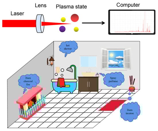
Figure 1.
Schematic diagram of the experimental system.
2.2. Sampling Modes
Four thousand bits of data were acquired for data accuracy and split into four portions, each lasting 2 min. Unlike the detection of solids, the detection of air signals is heavily influenced by a variety of variables, including the non-uniformity of the created aerosols, which results in a significant number of single values in the spectrum signal. To address the primary challenge of interference signals, isolated forest was employed to facilitate later classification and neural network design. To screen out single values, isolated forests are frequently employed in outlier testing [22]. When constructing an isolated forest, two parameters need to be set: the number of trees t and the maximum value of sample size per tree sampled Ψ. According to Liu et al. on isolated forest, the t is set to 100 and the Ψ is set to 256 as the optimal screening condition [23]. The isolated forest mainly relies on the anomaly function s(x,n) to determine whether the data is an outlier, which is shown in Equations (1)–(3)
where E(h(x)) is the expected value of the path length of x in multiple trees, c(n) is the average path length of the tree for a data set containing n samples, is the harmonic number, and is the Euler constant, which is about 0.57. Normally, s (x,n) is less than 0.8, and the closer s (x,n) is closer to 1, the higher the possibility of a data anomaly. The spectra exhibited matched to a single shot, and after screening, 400 well-performing spectral samples with high dynamic qualities were produced for each sample. As a result, a network analysis was developed using a large data source [24].
3. Results and Discussion
3.1. Analysis of Spectra
In this part, air was chosen as the experimental object in four scenarios to conduct the spectrum analysis. Table 1 shows the materials and compositions utilized in the four simulation situations. The air spectrum was initially measured under normal conditions, as shown in Figure 2a, and was then utilized to imitate normal interior air conditions. According to the National Institute of Standards and Technology (NIST) [25], a substance’s composition can be well stated in a certain range of wavelengths. As a result, at a later stage of the experiment, the indoor air spectrum was utilized as a criterion for detecting component changes.

Table 1.
Experimental materials.
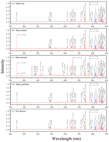
Figure 2.
(a) Spectra (200 nm to 890 nm) of indoor air; (b) Spectra (200 nm to 890 nm) of burning carbon; (c) Spectra (200 nm to 890 nm) of burning incense; (d) Spectra (200 nm to 890 nm) of spraying perfume; (e) Spectra (200 nm to 890 nm) of hot shower.
Data standardization was utilized to make the spectrum among distinct scenes more visible. By reducing the intensity of the n to the unit 1, all the intensities were processed by this criterion. To make sure the accuracy of the spectral data and get rid of the factor of time variation, as soon as the measurement began, the spectral data in the first minute was chosen as a static measurement. Spectral information of four scenarios is illustrated in Figure 2b–e, where the spectral lines of major elements correspond to C I 247.86 nm and Hα 656.28 nm [26,27,28,29]. Through observing, it shows that indoor air and hot shower obtained the lowest C intensity, while spraying perfume had a higher C intensity than indoor air. The highest value came from what gas generated by burning carbon, which was almost seven times that of the indoor air. As known to all, charcoal contains a high concentration of carbon and produces a large amount of carbon monoxide and carbon dioxide after combustion [30,31,32,33,34,35]. Those combustion products can badly harm the natural environment, and even seriously threaten human health within a confined area [36]. These all indicate the importance of ventilation in the home. In addition, from the Hα spectral line, it was observed that indoor air and burning carbon presented the same H intensity. However, the main ingredient of perfume is alcohol, leading to a higher H intensity compared with indoor air [37,38]. Similarly, a hot shower also resulted in an increment of H, which was approximately two times that of the indoor air. It is worth mentioning that despite the difference in the intensity of H, a hot shower obtained the same spectrum as indoor air, revealing the existence of a small difference in their compositions. This happened when spraying perfume and burning carbon: except for the H intensity, which varied minimally in burning carbon, their components altered in the same way. Furthermore, in the scenario of burning incense, which had the highest H intensity, the content of H grew with the appearance of metal elements, and the intensity of H reached a spectral maximum, which was consistent with the finding of element O. It is worth mentioning that the metal elements produced by burning incense are innocuous in minor quantities, such as iron, calcium and sodium, but if burned in excess over a long period of time, the accumulation of metal elements can lead to poisoning of the body.
Normally, the difference in environments can be distinguished rapidly by human beings through direct observation. For example, there may be a high concentration of C in an environment with smoke or a high concentration of H in an environment with water. However, it gets more difficult when the settings to be compared share the same physical shape. As is well known, aerosols may be formed in both the carbon and incense burning processes. The former creates aerosols mostly composed of C [39,40,41,42]. Conversely, as compared to burning carbon, incense creates several metal elements. Spraying perfume and taking a hot shower both create droplets in the same condition. According to the findings, the LIBS technology, which has the properties of analyzing quickly and being unaffected by matter form, can distinguish the composition of diverse chemicals, indicating possible applications in environmental detection.
3.2. PCA and KNN of Experimental Results
It is without debate that automated identification of air quality in varied settings is a vital step in environmental detection [43,44,45]. The categorization of chemicals is a key part of automated identification. However, there are severe obstacles in the classification of gases. Because the signal’s ambiguity made classification more difficult, PCA and KNN were utilized for air environment classification based on isolated forest data processing. When compared to other analysis methods such as random forest, PCA provides faster operation speed and more straightforward and obvious findings [46]. As a result, PCA is frequently utilized as a vital technique in automated recognition.
Numerous scientific studies need the processing of data with many variables. Because there may be correlations between outcomes, analyzing only one variable will result in an inadequate use of the data, neglecting some of the relationships. However, analyzing a large number of variables at once increases the process’s complexity. PCA technology was created in response to the aforementioned issues. Dimension reduction, or maintaining some of the most relevant elements of high-dimensional data while deleting uninteresting information, is at the core of PCA. The entire data processing process is generally divided into six steps [47]: calculating the average of the variable, calculating the dispersion, calculating the covariance of the variable, constructing a covariance matrix, calculating the eigenvalues, and sorting by size and computing feature vectors, respectively.
However, the PCA is not suitable for the processing of all the data. In this research, the Kaiser-Meyer-Olkin (KMO) and Bartlett test, a method to determine whether the data dimension can be reduced, was employed. As illustrated by Equations (4) and (5) where MSe represents the average error, Si2 is the standard deviation and r represents the number of datasets.
When the KMO value is more than 0.6 and the p value is less than 0.005, the data can be disposed by PCA. A total of 400 well-performing spectral data for each sample were utilized for PCA analysis. The important bands of 280 to 350 nm, 300 to 500 nm and 550 to 800 nm in the spectrum of each sample were reserved for PCA analysis. All the above operations were completed via the MATLAB R2019B software of the personal computer [48]. The experimental data of four scenarios and indoor air were calculated, with the results shown in Table 2 (a). According to the spectral results acquired before, these five categories of data were not suited for PCA. The spectral makeup of a hot shower was the same as that of indoor air. Spraying perfume also had the same spectral composition as burning carbon. As a consequence, the data from spraying perfume and hot showers were recalculated as burning carbon and indoor air, respectively, with the findings shown in Table 2 (b). There is no doubt that these three sets of data matched the PCA criteria flawlessly.
Table 2.
KMO and Bartlett Test.
The scree test, which refers to an intuitive PCA plot, shows how many factors are present in the analyzed data. In addition, it also represents the quantity of the variable information covered by the components. In general, it is steep first and then gradually drops, with the first element encompassing the greatest amount of information and then decreasing in turn. When the eigenvalues tend to be flattened, the abscissa relates to the number of components. As seen in Figure 3, when the third component is extracted, it may effectively encompass all of the information of the original variable, indicating that the data can be reduced to three dimensions.
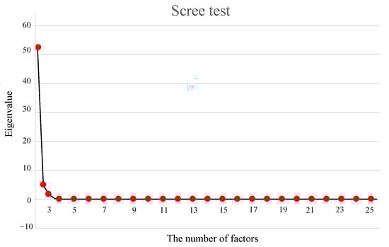
Figure 3.
Scree test of the three scenarios in the experiment.
Figure 4a presents a 3D PCA figure of the data from the experiment, where the experimental data for the three situations is obviously split into three groups. Additionally, Figure 4b shows a 2D plot of the XY surface, and Table 3 shows some of the partial PC band weights.
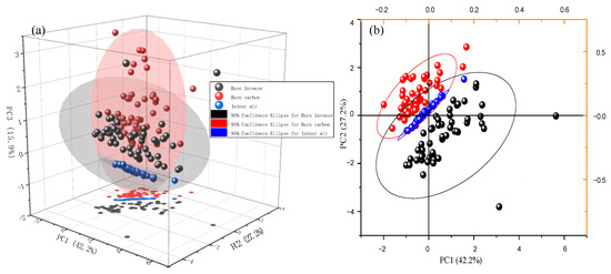
Figure 4.
(a) The 3D result of PCA including indoor air, burning carbon and burning incense; (b) The 2D result of PCA including indoor air, burning carbon and burning incense.
Table 3.
Partial PC band weights.
As seen in Figure 4a, there is little doubt that the interior air does not connect with the other two scenarios. This is because the PC3 axis has a large weight at 247 nm, which corresponds to the spectral intensity of carbon. At the same time, it is clear that the PC3 axis has less impact on the two scenarios, which include burning carbon and burning incense, and it implies that PC1 and PC2 are crucial.
KNN was utilized for scene classification using PCA’s dimensionality reduction data processing. To lessen the influence of the received spectral signal strength, the data was normalized in terms of the intensity of the n element during data processing. The KNN processing comprised 400 data sets for each scenario, with 265 training data and 135 testing data sets. From the PCA results, it can be seen that the factors determining the differences between the three scenes can be extracted as three factors, which correspond to 247 nm–249 nm, 587 nm–560 nm and 655 nm–657 nm, respectively. Therefore, partial spectra rather than whole spectra were used in the KNN classification. As shown in Figure 5a, the confusion matrix of the training data indicates that the accuracy of training is 0.996. Meanwhile, Figure 5b shows the confusion matrix of the test data, where the classification accuracy of the test data is 0.992.
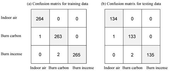
Figure 5.
(a) Confusion matrix for training data; (b) confusion matrix for testing data.
The results of KNN show that the three types of air can be classified with high precision. Since the component of C element plays a major role in PCA reduction, the air classification can be named as follows: normal air which represents air with low carbon content, air with high carbon content and air with high heavy metal content. Obviously, they correspond to the three scenarios: indoor air, burning carbon and burning incense, respectively. The results are also not surprising and show that burning incense produces the greatest effect on air composition. In the experiment, there was carbon aerosol in the air after burning carbon and there was a large amount of smoke in the air after burning incense, which was completely compatible with the results obtained from our actual data processing.
Existing KNN analysis data could be put into the database to determine the aerosol composition in the environment more quickly. Differentiated by carbon concentration size, Low carbon content environments, and high carbon content environments are constructed to be different scenarios. When new aerosols occur, they may be examined in the database for the same or comparable data, which can help determine their composition more rapidly.
3.3. Neural Network
Neural network prediction is a practical tool in machine learning [49,50,51]. It operates by training the supplied sample data and employing machine learning algorithms to discover a link between input and output. When fresh data is entered, the appropriate output, referred to as the prediction result, may be derived using the procedures outlined above [52,53].
Time and element concentration may be connected using the neural network, allowing for dynamic prediction of element concentration. Previous studies indicated an explicit link between material concentration and spectral signal strength [54]. Thus, the relation between spectral intensity and element content can be assumed with Equation (6).
IC is the spectral signal intensity of carbon, nC is the carbon concentration, M is a quantity determined by the environment, α and β are constants. In the ideal case, other disturbances such as self-absorption of spectral lines are ignored, which makes M = 0. Therefore, there exists a linear relationship between lnIC and lnnC. The carbon element has long been a critical topic for the environment research; therefore, a model for burning carbon was chosen and a neural network based on the variation of carbon intensity with time was built [55]. Under normal conditions, the carbon source of indoor air is carbon dioxide and its concentration is not worth mentioning compared with burning carbon. Therefore, the carbon dioxide in the original air was ignored when the carbon concentration model was established. The concentration of carbon dioxide in the room is about 300 ppm, and the carbon concentration in general air is considered to be 0.03% [56]. The indoor air spectral lines were obtained by LIBS in 8 min, which had 4000 pieces of data. The statistics of the carbon spectral line intensity values were obtained: the mean value is 362 which stands the intensity of the carbon spectral line in the indoor air can be expressed as 362. According to the study researched by Koenig, it is beyond dispute that the carbon concentration in exhaled air was 4.0% and the spectral line signal intensity value was 4902 [57]. Thus, β could be calculated to be −0.47 and α is 11.26. There is no doubt that carbon concentration and spectral intensity models have been developed, such as Equation (7).
According to Equation (7), the carbon concentration achieves a connection with the carbon spectral intensity. Therefore, no matter how small the spectral intensity is, the concentration can be deduced. The neural network technique used 400 pieces of data in total, 200 for training, 100 for validation, and 100 for testing. The BP neural network approach was used to calculate in this machine learning. The neural network’s architecture, which created a chain-shaped cross structure, was established in the input layer, the hidden layer, and the output layer. In addition, 6 hidden layers and 5 nodes were built. The neural network fitting result of this experiment is shown in Figure 6a, where the Train line represents the algorithm fitting process inside the system and the Validation line shows the data produced by the system automatically based on the training results for the prediction. Evidently, after 24 epochs of training, the validation curve corresponded with the train curve, indicating that the neural network was successfully constructed. However, the correlation coefficient was calculated to be 0.8813, and the test curve did not agree with the other two curves, suggesting that errors in the projected outcome were present. According to Table 4, some experimental data was used to compute the neural network’s mistakes. Figure 6b depicts the prediction result, demonstrating the practical usefulness of this machine learning. The overall accuracy of the seven selected data points was 96.5 percent, and Figure 7 shows the error bars of the BP neural network predictions. It is worth mentioning that the quantitative analysis of any element can be modeled with high accuracy in the mentioned way for the conversion of spectral intensity to concentration. Therefore, the indoor environment can be equipped with a device containing machine learning to detect the composition at any time to warn of whether a substance will exceed the threshold in the future.
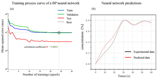
Figure 6.
(a) Training process curve of a BP neural network; (b) neural network predictions.
Table 4.
Neural network prediction of elemental concentrations.
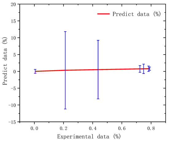
Figure 7.
Error bars of BP neural network predictions.
4. Conclusions
Experiments were carried out in four scenarios based on LIBS to determine indoor air quality, and related plasma emission spectra were acquired. The atomic lines of common elements such as C, H, and O were clearly seen. Through observing, it shows that burning carbon added a significant amount of carbon to the air as compared to inside air, but burning incense added more metal elements. LIBS-based environmental detection successfully and quickly identified cases with the same physical condition. The PCA was then paired with spectra to investigate the air composition connection in diverse situations. The isolated forest was employed to deal with the consequences of signal strength detection. Upon that basis, the four situations were classified as normal air, air having a high concentration of carbon, and air containing a high concentration of metal elements with 99.2 percent accuracy using the KNN algorithm, giving a reference for the database’s creation. Ultimately, for the first time, a high-precision quantitative detection model for carbon content in an indoor setting was developed. The prediction of air composition concentrations was carried out using the neural network method in order to comprehend the dynamic features of situations, and the forecast accuracy of carbon elements in the experiment was 96.5 percent. In conclusion, the experimental data and results demonstrate the feasibility of using LIBS technology and machine learning technology to detect air quality and predict air composition concentrations, which can provide a reference for future air quality research.
Author Contributions
This article was written by a total of five authors, each of whom made the following major contributions: conceptualization, X.Z. and Z.Z.; methodology, X.Z.; software, X.Z.; validation, Z.Z., Z.S. and Y.L.; formal analysis, X.Z.; resources, Z.S.; data curation, X.Z.; writing—original draft preparation, X.Z.; writing—review and editing, X.Z. and S.J. All authors have read and agreed to the published version of the manuscript.
Funding
This research was funded by National Natural Science Foundation of China (U1932149) and NUIST Students’ Platform for Innovation and Entrepreneurship Training Program (202210300134Y).
Institutional Review Board Statement
Not applicable.
Informed Consent Statement
Not applicable.
Data Availability Statement
No data provided.
Acknowledgments
The authors are grateful to Ziang Chen for his support in language polishing.
Conflicts of Interest
We declare that we have no financial and personal relationships with other people or organizations that can inappropriately influence our work, and there is no professional or other personal interest of any nature or kind in any product, service and/or company that could be construed as influencing the position presented in, or the review of, the manuscript entitled “Analysis and dynamic monitoring of indoor air quality based on laser-induced breakdown spectroscopy and machine learning”, by X.Z., Z.S., Z.Z., S.J. and Y.L.
References
- Al-Kindi, S.G.; Brook, R.D.; Biswal, S. Environmental determinants of cardiovascular disease: Lessons learned from air pollution. Nat. Rev. Cardiol. 2020, 17, 656. [Google Scholar] [CrossRef]
- Kim, S.Y.; Kim, S.H.; Wee, J.H. Short- and long-term exposure to air pollution increases the risk of ischemic heart disease. Sci. Rep. 2021, 11, 5108. [Google Scholar] [CrossRef]
- Lee, D.H.; Han, J.; Jang, M. Association between Meniere’s disease and air pollution in South Korea. Sci. Rep. 2021, 11, 13128. [Google Scholar] [CrossRef]
- Qu, Y.; Zhang, Q.; Yin, W.; Hu, Y.; Liu, Y. Real-time in situ detection of the local air pollution with laser-induced breakdown spectroscopy. Optics Express, 27(12), pp.A790-A799. Real-time in situ detection of the local air pollution with laser-induced breakdown spectroscopy. Opt. Express 2019, 27, 790. [Google Scholar] [CrossRef]
- Gupta, A.; Goyal, R.; Kulshreshtha, P. Environmental and of Delhi, CO2 India in Indoor Monitoring Office Spaces of PM2.5. Indoor Environ. Qual. Sel. Proc. 1st ACIEQ 2020, 60, 67. [Google Scholar]
- Passi, A.; Nagendra, S.M.S.; Maiya, M.P. Characteristics of indoor air quality in underground metro stations: A critical review. Build. Environ. 2021, 198, 107907. [Google Scholar] [CrossRef]
- Zhang, X.; Luo, G.; Xie, J. Associations of bedroom air temperature and CO2 concentration with subjective perceptions and sleep quality during transition seasons. Indoor Air 2021, 31, 1004. [Google Scholar] [CrossRef] [PubMed]
- Zhang, Y.; Zhang, T.; Li, H. Application of laser-induced breakdown spectroscopy (LIBS) in environmental monitoring. Spectrochim. Acta Part B At. Spectrosc. 2021, 181, 106218. [Google Scholar] [CrossRef]
- Ikeda, Y.; Kawahara, N. Measurement of Cyclic Variation of the Air-to-Fuel Ratio of Exhaust Gas in an SI Engine by Laser-Induced Breakdown Spectroscopy. Energies 2022, 15, 3053. [Google Scholar] [CrossRef]
- Minchero, M.M.; Ulloa, L.; Cobo, A. Laser-induced breakdown spectroscopy analysis of copper and nickel in chelating resins for metal recovery in wastewater. Spectrochim. Acta Part B At. Spectrosc. 2021, 180, 106170. [Google Scholar] [CrossRef]
- Yue, Z.; Sun, C.; Chen, F.; Zhang, Y.; Xu, W.; Shabbir, S.; Zou, L.; Lu, W.; Wang, W.; Xie, Z.; et al. Machine learning-based LIBS spectrum analysis of human blood plasma allows ovarian cancer diagnosis. Biomed. Opt. Express 2021, 12, 2559. [Google Scholar] [CrossRef] [PubMed]
- Gaudiuso, R.; Ewusi-Annan, E.; Melikechi, N.; Sun, X.; Liu, B.; Campesato, L.F.; Merghoub, T. Using LIBS to diagnose melanoma in biomedical fluids deposited on solid substrates: Limits of direct spectral analysis and capability of machine learning. Spectrochim. Acta Part B At. Spectrosc. 2018, 146, 106. [Google Scholar] [CrossRef]
- Berlo, K.; Xia, W.; Zwillich, F.; Gibbons, E.; Gaudiuso, R.; Ewusi-Annan, E.; Chiklis, G.R.; Melikechi, N. Laser induced breakdown spectroscopy for the rapid detection of SARS-CoV-2 immune response in plasma. Sci. Rep. 2022, 12, 1614. [Google Scholar] [CrossRef] [PubMed]
- Sabsabi, M.; Cielo, P. Quantitative analysis of aluminum alloys by laser-induced breakdown spectroscopy and plasma characterization. Appl. Spectrosc. 1995, 49, 499. [Google Scholar] [CrossRef]
- Anglos, D. Laser-induced breakdown spectroscopy in art and archaeology. Appl. Spectrosc. 2001, 55, 186. [Google Scholar] [CrossRef]
- Killiny, N.; Etxeberria, E.; Flores, A.P.; Blanco, P.G. Laser-induced breakdown spectroscopy (LIBS) as a novel technique for detecting bacterial infection in insects. Sci. Rep. 2019, 9, 2449. [Google Scholar] [CrossRef] [Green Version]
- Jang, S.Y.; Han, S.H. Fabrication of si negative electrodes for li-ion batteries (LIBS) using cross-linked polymer binders. Sci. Rep. 2016, 6, 38050. [Google Scholar] [CrossRef] [Green Version]
- Foster, J.D.; Osterink, L.M. Thermal effects in a Nd:YAG laser. J. Appl. Phys. 1970, 41, 3656. [Google Scholar] [CrossRef]
- Fan, T.Y. Heat generation in Nd:YAG and Yb: YAG. IEEE J. Quantum Electron. 1993, 29, 1457. [Google Scholar] [CrossRef]
- Lu, J.; Prabhu, M.; Song, J. Optical properties and highly efficient laser oscillation of Nd:YAG ceramics. Appl. Phys. B 2000, 71, 469. [Google Scholar] [CrossRef]
- Zhou, B.; Kane, T.J.; Dixon, G.J. Efficient, frequency-stable laser-diode-pumped Nd:YAG laser. Opt. Lett. 1985, 10, 62. [Google Scholar] [CrossRef] [PubMed]
- Wang, Z.; Afgan, M.S.; Gu, W.; Song, Y.; Wang, Y.; Hou, Z.; Song, W.; Li, Z. Recent advances in laser-induced breakdown spectroscopy quantification: From fundamental understanding to data processing. TrAC Trends Anal. Chem. 2021, 143, 116385. [Google Scholar] [CrossRef]
- Liu, F.T.; Ting, K.M.; Zhou, Z.H. Isolation Forest. In Proceedings of the 2008 Eighth IEEE International Conference on Data Mining, Pisa, Italy, 15–19 December 2008; IEEE: Piscataway, NJ, USA, 2008; p. 413. [Google Scholar]
- Corel, E.; Lopez, P.; Méheust, R.; Bapteste, E. Network-thinking: Graphs to analyze microbial complexity and evolution. Trends Microbiol. 2016, 24, 224. [Google Scholar] [CrossRef] [PubMed]
- Gentile, T.R.; Houston, J.M.; Hardis, J.E. National Institute of Standards and Technology high-accuracy cryogenic radiometer. Appl. Opt. 1996, 35, 1056. [Google Scholar] [CrossRef] [PubMed]
- Peng, J.; Song, K.; Zhu, H. Fast detection of tobacco mosaic virus infected tobacco using laser-induced breakdown spectroscopy. Sci. Rep. 2017, 7, 44551. [Google Scholar] [CrossRef]
- Lee, J.H.; Giannikopoulos, P.; Duncan, S.A. The transcription factor cyclic AMP–responsive element–binding protein H regulates triglyceride metabolism. Nat. Med. 2011, 17, 812. [Google Scholar] [CrossRef] [Green Version]
- Zhou, J.; Chizhik, A.I. Single-particle spectroscopy for functional nanomaterials. Nature 2020, 579, 41. [Google Scholar] [CrossRef]
- Brixner, T.; Stenger, J.; Vaswani, H.M. Two-dimensional spectroscopy of electronic couplings in photosynthesis. Nature 2005, 434, 625. [Google Scholar] [CrossRef]
- Sakakura, T.; Choi, J.C.; Yasuda, H. Transformation of carbon dioxide. Chem. Rev. 2007, 107, 2365. [Google Scholar] [CrossRef]
- Schmalensee, R.; Stoker, T.M.; Judson, R.A. World carbon dioxide emissions: 1950–2050. Rev. Econ. Stat. 1998, 80, 15. [Google Scholar] [CrossRef]
- Siegenthaler, U.; Sarmiento, J.L. Atmospheric carbon dioxide and the ocean. Nature 1993, 365, 119. [Google Scholar] [CrossRef]
- Lim, X.Z. How to make the most of carbon dioxide. Nature 2015, 526, 628. [Google Scholar] [CrossRef] [PubMed] [Green Version]
- Alessandro, D.; Smit, B.; Long, J.R. Carbon dioxide capture: Prospects for new materials. Angew. Chem. Int. Ed. 2010, 49, 6058. [Google Scholar] [CrossRef] [Green Version]
- Fenghour, A.; Wakeham, W.A.; Vesovic, V. The viscosity of carbon dioxide. J. Phys. Chem. Ref. Data 1998, 27, 31. [Google Scholar] [CrossRef]
- Jacobson, T.A.; Kler, J.S. Direct human health risks of increased atmospheric carbon dioxide. Nat. Sustain. 2019, 2, 691. [Google Scholar] [CrossRef]
- Brand, P.; Hinojosa-Díaz, I.A.; Ayala, R. The evolution of sexual signaling is linked to odorant receptor tuning in perfume-collecting orchid bees. Nat. Commun. 2020, 11, 244. [Google Scholar] [CrossRef] [PubMed] [Green Version]
- Carlos, L.J. Two steps closer to the ultimate perfume. Nat. Rev. Neurosci. 2000, 1, 4. [Google Scholar] [CrossRef]
- Cousins, R.J. Metal elements and gene expression. Annu. Rev. Nutr. 1994, 14, 449. [Google Scholar] [CrossRef]
- Waldron, K.J.; Rutherford, J.C.; Ford, D. Metalloproteins and metal sensing. Nature 2009, 460, 823. [Google Scholar] [CrossRef]
- Gutiérrez-Gutiérrez, S.C.; Coulon, F.; Jiang, Y. Rare earth elements and critical metal content of extracted landfilled material and potential recovery opportunities. Waste Manag. 2015, 42, 128. [Google Scholar] [CrossRef]
- Starukh, H.; Praus, P. Doping of graphitic carbon nitride with non-metal elements and its applications in photocatalysis. Catalysts 2020, 10, 1119. [Google Scholar] [CrossRef]
- Wold, S.; Esbensen, K.; Geladi, P. Principal component analysis. Chemom. Intell. Lab. Syst. 1987, 2, 37. [Google Scholar] [CrossRef]
- Abdi, H.; Williams, L.J. Principal component analysis. Wiley Interdiscip. Rev. Comput. Stat. 2010, 2, 433. [Google Scholar] [CrossRef]
- Ringnér, M. What is principal component analysis? Nat. Biotechnol. 2008, 26, 303. [Google Scholar] [CrossRef]
- Nitze, I.; Schulthess, U.; Asche, H. Comparison of Machine Learning Algorithms Random Forest, Artificial Neural Network and Support Vector Machine to Maximum Likelihood for Supervised Crop Type Classification. In Proceedings of the 4th GEOBIA, Rio de Janeiro, Brazil, 7–9 May 2012; Volume 79, p. 3540. [Google Scholar]
- Lever, J.; Krzywinski, M.; Altman, N. Points of significance: Principal component analysis. Nat. Methods 2017, 14, 641. [Google Scholar] [CrossRef] [Green Version]
- Higham, D.J.; Higham, N.J. MATLAB Guide; Society for Industrial and Applied Mathematics: Philadelphia, PA, USA, 2016. [Google Scholar]
- Leshno, M.; Spector, Y. Neural network prediction analysis: The bankruptcy case. Neurocomputing 1996, 10, 125. [Google Scholar] [CrossRef]
- Raghunath, S.; Ulloa, A.E. Prediction of mortality from 12-lead electrocardiogram voltage data using a deep neural network. Nat. Med. 2020, 26, 886. [Google Scholar] [CrossRef]
- Lotter, W.; Kreiman, G.; Cox, D. A neural network trained for prediction mimics diverse features of biological neurons and perception. Nat. Mach. Intell. 2020, 2, 210. [Google Scholar] [CrossRef]
- Li, A.; Chen, R.; Farimani, A.B. Reaction diffusion system prediction based on convolutional neural network. Sci. Rep. 2020, 10, 3894. [Google Scholar] [CrossRef] [Green Version]
- Senior, A.W.; Evans, R.; Jumper, J. Improved protein structure prediction using potentials from deep learning. Nature 2020, 577, 706. [Google Scholar] [CrossRef]
- Taganov, K.I.; Travina, V.G. Some relations between spectral line intensities and the power and concentration of materials in light sources. Appl. Spectrosc. 1971, 15, 841. [Google Scholar] [CrossRef]
- Murari, G.F.; Penido, J.A.; Machado, P.A.L.; de Lemos, L.R.; Lemes, N.H.T.; Virtuoso, L.S.; Rodrigues, G.D.; Mageste, A.B. Phase diagrams of aqueous two-phase systems formed by polyethylene glycol+ ammonium sulfate+ water: Equilibrium data and thermodynamic modeling. Fluid Phase Equilibria 2015, 406, 61. [Google Scholar] [CrossRef]
- Hewitt, R. Air Composition and Chemistry.by Peter Brimblecombe. Appl. Ecol. 1987, 24, 327. [Google Scholar] [CrossRef]
- Koenig, T.S.; Synal, W.H.A. Direct radiocarbon analysis of exhaled air. Anal. At. Spectrom. 2011, 26, 287. [Google Scholar] [CrossRef]
Publisher’s Note: MDPI stays neutral with regard to jurisdictional claims in published maps and institutional affiliations. |
© 2022 by the authors. Licensee MDPI, Basel, Switzerland. This article is an open access article distributed under the terms and conditions of the Creative Commons Attribution (CC BY) license (https://creativecommons.org/licenses/by/4.0/).