Comparison of Various Signal Processing Techniques and Spectral Regions for the Direct Determination of Syrup Adulterants in Honey Using Fourier Transform Infrared Spectroscopy and Chemometrics

Abstract

Honey consumption has become increasingly popular worldwide. However, the increase in demand for honey has also caused an increase in its adulteration, a deliberate fraud which involves adding of other substances to pure honey for economic purposes. This process not only lowers the quality of honey, but also has potential health risks, including high blood sugar, increased risk of diabetes, and weight gain. Herein, we develop an easy-to-use and direct method of quantifying corn, cane, beet, and rice syrup adulterants in honey using Fourier transform infrared spectroscopy and chemometrics. Various signal processing techniques, including derivatives, moving average, binning, Savitzky–Golay, and standard normal variate using the entire spectral region (3996–650 cm⁻¹) and specific spectral region (1501–799 cm⁻¹), were compared. Optimum results were obtained using first derivative signal processing for both the entire and specific spectral regions. The first derivative signal processing technique garnered the most optimum results using the specific spectral range (1501–799 cm⁻¹) (RMSECV_average = 0.021, RMSEP_average = 0.014, R²_average = 0.859) across all syrup adulterants. An exploratory analysis to assess the utility of this specific spectral region in pattern recognition of samples based on their adulterant content show that this region is effective in discriminating samples according to the presence or absence of honey syrup adulterants.

1. Introduction

Honey is a thick, sugary, concentrated nectar that is made up of approximately 18% water. Due to its sweet and sticky texture, honey has found itself as a staple ingredient in many kitchens. Aside from its culinary applications, honey also has several medical applications, e.g., it has both anti-aging and anti-bacterial properties and can also be used as a remedy for sore throat. As the human population grows, the consumption of honey grows as well. However, the assessment of honey safety and quality is not regularly monitored. Further, due to its growing demand, adulteration has also become more common. In the case of honey, adulteration is the addition of any substance to the pure honey. Adulterants most frequently added to honey include syrups of corn, cane, beet, and rice, which have economic and organoleptic consequences. In addition, adulterated honey poses risks to consumer health, such as higher blood sugar and weight gain. Due to the decline in honey quality, consumers have perceived low confidence in the nutritional value this product brings, making its marketing to the public more challenging [1]. Honey evaluation would therefore not only help to improve the quality of honey, but also assist in improving its appeal to the public.

Previous studies have assessed the presence of syrup adulterants in honey but are primarily focused on improving the discrimination of adulterated honey from authentic ones [2]. Further, most studies were also focused on the rapid detection of sugar adulterants (e.g., D-fructose, D-glucose, etc.), a few syrup honey adulterants (i.e., one or two adulterant matrices), and in many cases using more expensive instrumentation, such as the nuclear magnetic resonance (NMR) spectrometer, high performance liquid chromatograph (HPLC), stable isotope ratio mass spectrometer, as well as a gas chromatograph-mass spectrometer (GC-MS) [3,4,5,6,7,8]. The use of the aforementioned techniques also requires good operational skills in handling these instruments [9]. The use of thin layer chromatography is another method proposed for honey adulteration detection and although has advantages of simplicity and speediness, extensive work is still needed to assess its reliability [9]. The use of the mid-infrared region (4000–400 cm⁻¹) associated with chemometrics has shown to be an accurate and fast method to detect and predict food adulteration [10]. For chemometrics, the use of partial least squares (PLS) regression is of particular interest because, unlike multiple linear regression, it has the ability to analyze data which are noisy, redundant, and strongly correlated [11]. Principal component analysis (PCA) is another chemometric technique that is used extensively for screening, extracting, and compressing multivariate data [12,13]. The main goal of these chemometric methods in conjunction with spectroscopic techniques is to develop an inexpensive, less time consuming, and easy to use application method to measure a property of interest in new and unknown samples [12,13]. In this study, we explored the utility of a Fourier transform infrared spectroscopy with attenuated total reflectance accessory (ATR-FTIR), which harbors the mid-IR region, and the PLS chemometric technique to simultaneously determine the concentrations of corn, cane, beet, and rice syrup adulterants in honey. ATR-FTIR offers several advantages over the other aforementioned techniques, such as the NMR, HPLC, and GC-MS. First, analysis using ATR-FTIR is very rapid and allows up to 100 samples to be analyzed per day. In addition, this method is easy to deploy, non-destructive to samples, requires a minimal sample as well as preparation, and is considered affordable compared to other methods.

In order to simultaneously determine the content of various syrup adulterants in honey, we implemented several multiple signal processing techniques, including first derivative, second derivative, moving average, binning, Savitzky–Golay, and standard normal variate (SNV) to both the entire (3996–650 cm⁻¹) and specific spectral regions (1501–799 cm⁻¹) harboring absorption bands of our samples of interest. This is the first study to perform a comprehensive examination and comparison of various signal processing techniques as applied to both the aforementioned spectral regions in honey.

2. Materials and Methods

A training set of adulterated honey samples (n = 81) containing various levels of corn, cane, beet, and rice syrups was created using a full factorial design (Table S1). A full factorial design creates experimental points using all the possible combinations of the levels of the factors. Thus, for four factors (i.e., components) having three levels of each factor considering a factorial design, a total of 3⁴ = 81 numbers of experiments were carried out. Similarly, an independent test set consisting of adulterated honey samples (n = 32) was created using a central composite design of experiments (Table S2). The DoE.base and rsm packages under the R Program were used to create the full factorial and central composite designs, respectively [14,15,16]. Pure Manuka honey was used as the base matrix and each sample syrup was weighed separately, then added to the pure honey and mixed thoroughly. A drop of each sample mixture was analyzed using a Bruker Tensor 27 ATR-FTIR with ZnSe crystal. Background spectra were collected using air as a blank and data collection was performed at every 2 cm⁻¹ resolution. Each sample was analyzed using 40 scans. The ATR crystal was carefully cleaned between analysis using ethanol and then allowed to air dry. The cleaned crystal was then checked spectrally prior to each analysis to ensure that no residue from previous sample analysis was retained. All spectral analyses were collected in triplicates and the average of the results was used for both the calibration and testing sets.

A PLS predictive model was built using data from the full-factorial training set using the ‘pls’ package in R [17]. The ultimate goal of PLS is to develop predictive models that will utilize the ATR-FTIR absorbance spectra to simultaneously predict the concentrations of corn, cane, beet, and rice syrups without any need for analytical separations. It is a powerful multivariate statistical method with a wide multitude of successes in many areas [18,19,20,21]. Mathematically, PLS involves the decomposition of A (absorbance) and C (concentration) as follows:

$$A=B{P}^T+E$$

(1)

$$C=D{Q}^T+F$$

(2)

where B and D are the n x d score matrices; P are the p x d loadings of the A matrix; E is the n x p error (residual) of A matrix; Q is the m x d loadings of the C matrix; and F is the n x m error (residual) of the C matrix. Computation of the B-coefficients is then given by:

$$B=W{(P^{T}W)}^{-1}{Q}^T$$

(3)

where W is a d × p matrix of PLS weights [22]. The central composite design testing set was developed as an independent dataset to test the accuracy of the predictive model created from the training data. All PLS analyses were performed using the R package ‘pls’ under RStudio [16]. Throughout the course of the PLS analysis, the PLS1 algorithm was utilized. PLS1 performs the optimization of the number of factors for only one component at a time [23].

Various signal processing techniques including Savitzky–Golay, binning, moving-average, first derivative, second derivative, and SNV were used to enhance the quality of the data by noise reduction, through the ‘ProspectR’ package [24].

Savitzky–Golay is a preprocessing technique that enhances signal properties, resolves overlapping signals, and suppresses unwanted spectral features arising due to nonideal instrument and sample properties [25]. It fits a local polynomial regression on the signal and requires equidistant bandwidth. Mathematically, it operates as a weighted sum of neighboring values [26].

$$x_j^{*}=\frac{1}{N}{\displaystyle \sum }_{h=-k}^k{c}_h$$

(4)

where $x_j^{*}$ is the new value, $N$ is a normalizing coefficient, $k$ is the gap size on each side of $j$, and $c_h$ are pre-computed coefficients that depend on the chosen polynomial order and degree [26,27,28]. A differentiation order of 1, polynomial order of 2, and a window size of 5 were used in all Savitzky–Golay analyses.

Binning is another preprocessing technique that averages a signal in column bins [26]. A top-down splitting technique, it is based on a specified number of bins and is primarily used for data smoothing [29]. Binning smooths a sorted data value by consulting neighboring values around it. The sorted values are then distributed into a number of “buckets” [30].

Moving-average, another robust signal processing technique performs a column-wise operation by averaging contiguous wavelengths within a given window size [26]. A filter length of 1 was used for the moving-average. First and second derivatives, on the other hand, were computed using the finite difference technique. In this method, the difference between subsequent data points was calculated provided that the band width is constant according to:

$$x_i^{\prime }=x_i-x_{i-1}$$

(5)

$$x_i^{″}=x_{i-1}-2\ast x_i+x_{i+1}$$

(6)

where $x_i^{\prime }$and $x_i^{″}$ are the new data points, and $x_i$, $x_{i-1}$, and $x_{i+1}$ are the subsequent data points [26].

SNV is another signal processing technique that normalizes spectra by correcting for light scattering through row-wise operation. Mathematically, it is given by:

$$SN{V}_i=\frac{x_i-\underset{\_}{\overline{x_i}}}{s_i}$$

(7)

where $x_i$ is the value of variable $i$, is the average of the variable $i$, and s_i is the standard deviation [26].

We assessed the performance of each signal processing technique comparing both the entire spectral (3996–650 cm⁻¹) and specific spectral regions (1501–799 cm⁻¹). Overall, there were 1736 datapoints (i.e., wavenumbers) used/adopted in the entire spectral region (3996–650 cm⁻¹) for all signal processing techniques. For the specific spectral region (1501–799 cm⁻¹), 365 datapoints (i.e., wavenumbers) were used/adopted.

After the training set was subjected to signal processing, PLS chemometric analysis was performed. The generated model from the training set (i.e., after cross-validation) was used to assess model performance in the validation data by predicting the sugar concentration ($\%\frac{w}{w})$ in the test set. Root mean square error (RMSE) was calculated to determine the degree to which the predicted concentrations of adulterants in the samples deviate from their actual concentrations in both the training and testing sets using the formula:

$$RMSE=\sqrt{\frac{{{\displaystyle \sum }}_{i=1}^N{(y_i-y_i^{\prime })}^2}{N}}$$

(8)

where y and y’ are the predicted and actual concentrations, respectively, and N is the number of samples [31]. The root mean square error of cross validation (RMSECV) and root mean square error of prediction (RMSEP) were both calculated for the training and testing datasets, respectively. Further, to determine the model’s goodness-of-fit between the measured and predicted adulterant concentrations, R² metrics were also calculated.

Lastly, PCA was then used to determine pattern recognition among samples in the specific spectral region harboring unique spectral peaks for the adulterants of interest. If a pattern was seen, then hierarchical cluster analysis was used to group together data points using the ‘ggbiplot’ R package [28]. In cluster analysis, the process starts with one piece of data and combines groups based on distances from one another in the principal component space [22]. The cluster analysis in this study was agglomerative hierarchical with Ward’s method used for the distances. PCA analysis was performed using the ‘factoextra’ R package [32,33].

3. Results and Discussion

Subtle spectral differences were evident in the fingerprint region (1501–500 cm⁻¹) in both the training and testing sets due to variations in the concentrations of the corn, cane, beet, and rice syrup adulterants (Figure 1 and Figure 2). These subtle spectral variations are critical aspects that allow discrimination of each respective syrup adulterants [34,35,36]. Beet syrup shows strong and unique absorbance bands in the 1101 cm⁻¹, 1053 cm⁻¹, 990 cm⁻¹, and 920 cm⁻¹ regions. Cane syrup, on the other hand, has similar absorbance bands to beet syrup. Corn syrup has absorbance bands at 1147 cm⁻¹, 1101 cm⁻¹, 1074 cm⁻¹, 1015 cm⁻¹, 991 cm⁻¹, and 920 cm⁻¹ [37,38]. Rice syrup has similar absorbance bands to cane syrup except for the absence of the prominent band at 991 cm⁻¹ [38]. Meanwhile, pure Manuka honey offers unique absorbance bands, particularly in the regions 1053 cm⁻¹, 1028 cm⁻¹, and 946 cm⁻¹ (Figure 3). In general, the region 1501–800 cm⁻¹ corresponds to the absorption zones of the three major sugar constituents of honey, namely glucose, fructose, and sucrose. Particularly, the region 900–750 cm⁻¹ corresponds to the anomeric region and is characteristic of the saccharide configurations [39]. The C-O and C-C stretching modes, on the other hand, are assigned in the bands 1153–904 cm⁻¹, while the O-C-H, C-C-H, and C-O-H angles due to the bending modes are assigned in the 1474–1199 cm⁻¹ absorption bands [40]. Water has an OH stretching peak that is intense, broad, and falls at ~3300 cm⁻¹ [41].

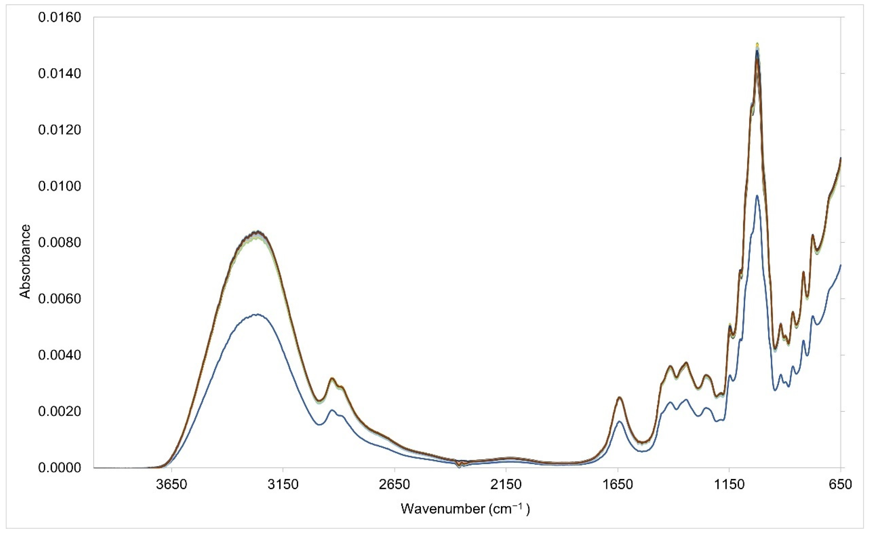
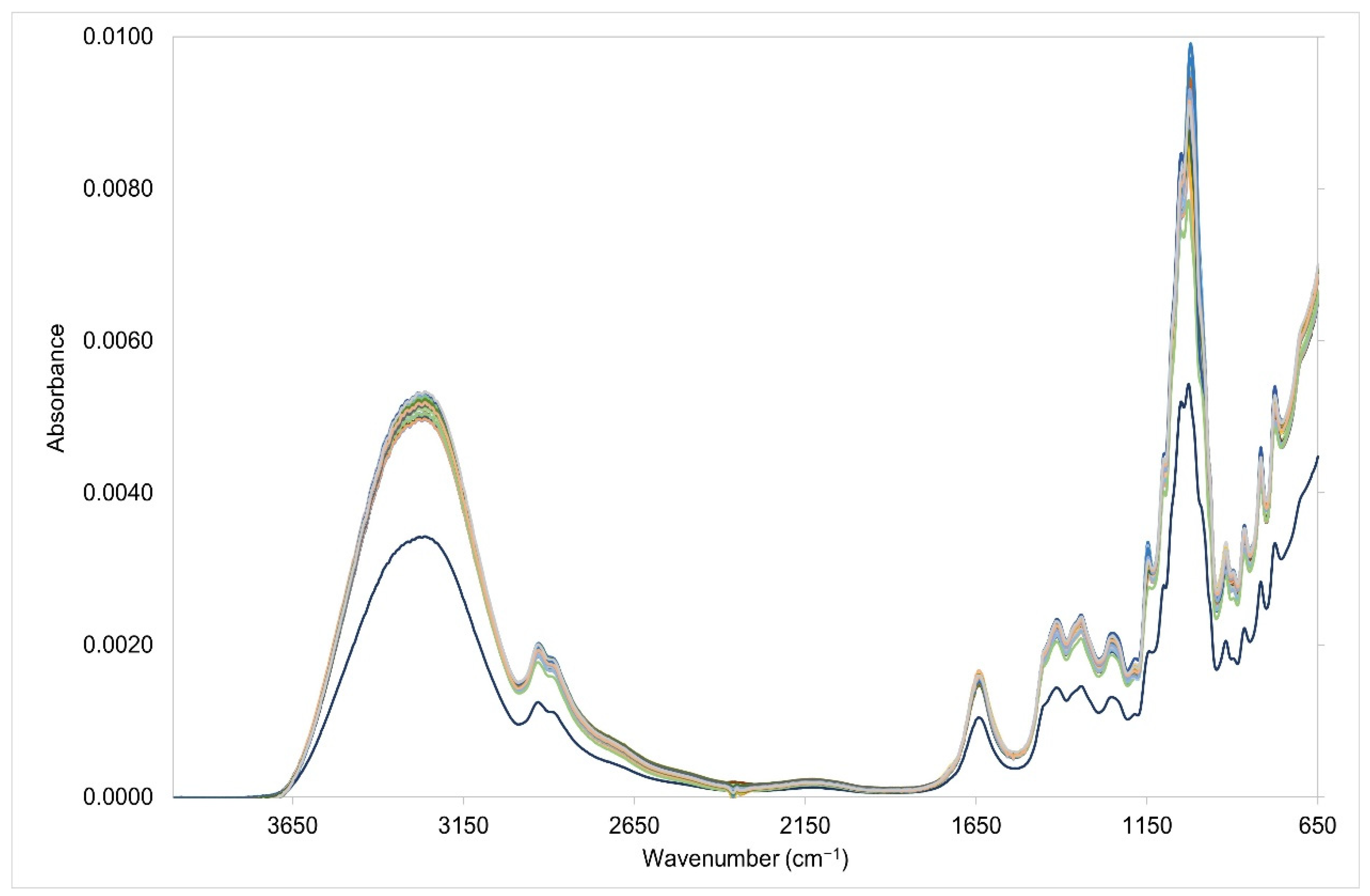
3.1. Analysis of the Entire Spectral Region (399–650 cm⁻¹)

In this study, we compared the performance of various signal preprocessing techniques using the entire spectral region (3996–650 cm⁻¹) and the specific spectral region (1501–799 cm⁻¹). We first attempted to perform a direct PLS analysis using the entire spectral region (3996–650 cm⁻¹) without any prior signal preprocessing technique. Our results for the training set for this particular region garnered RMSECV values of 0.030, 0.015, 0.019, and 0.031 for the corn, cane, beet, and rice syrups, respectively (${\mathrm{RMSECV}}_{\mathrm{average}}=0.024$) (

Table 1. Root mean square error of cross validation values for the full factorial training set (n = 81) showing the accuracy of the predicted model (PLS = partial least squares).

Techniques Performed	Signal Processing	Corn	Cane	Beet	Rice	Average
Signal processing and PLS analysis of entire spectral region (3996–650 cm−1)	No Pre-processing	0.030	0.015	0.019	0.031	0.024
	First Derivative	0.022	0.02	0.02	0.017	0.020
	Second Derivative	0.014	0.012	0.02	0.014	0.015
	Moving Average	0.030	0.015	0.019	0.031	0.024
	Binning	0.031	0.015	0.019	0.031	0.024
	Savitzky-Golay	0.042	0.018	0.016	0.035	0.028
	Standard Normal Variate	0.038	0.025	0.016	0.030	0.027
Signal processing and PLS analysis of specific spectral region (1501–799 cm−1)	No Pre-Processing	0.028	0.013	0.018	0.019	0.020
	First Derivative	0.022	0.024	0.023	0.015	0.021
	Second Derivative	0.016	0.021	0.030	0.018	0.021
	Moving Average	0.028	0.013	0.018	0.019	0.020
	Binning	0.029	0.014	0.018	0.02	0.020
	Savitzky-Golay	0.033	0.023	0.019	0.028	0.026
	Standard Normal Variate	0.029	0.018	0.025	0.021	0.023

). The corresponding R² values garnered an ${\mathrm{R}}_{\mathrm{average}}^2=0.824$ across these four syrup adulterants (

Table 2. R² values for the four syrup training set data indicating the goodness-of-fit measure for the predictive models (PLS = partial least squares).

Techniques Performed	Signal Processing	Corn	Cane	Beet	Rice	Average
Signal processing and PLS analysis of entire spectral region (3996–650 cm−1)	No Pre-processing	0.724	0.913	0.903	0.757	0.824
	First Derivative	0.858	0.845	0.891	0.925	0.880
	Second Derivative	0.943	0.938	0.897	0.948	0.932
	Moving Average	0.724	0.913	0.903	0.757	0.824
	Binning	0.722	0.912	0.902	0.756	0.823
	Savitzky-Golay	0.458	0.86	0.927	0.681	0.732
	Standard Normal Variate	0.579	0.741	0.931	0.763	0.754
Signal processing and PLS analysis of specific spectral region (1501–799 cm−1)	No Pre-Processing	0.759	0.926	0.914	0.903	0.876
	First Derivative	0.853	0.772	0.865	0.944	0.859
	Second Derivative	0.925	0.824	0.755	0.913	0.854
	Moving Average	0.759	0.926	0.914	0.903	0.876
	Binning	0.756	0.925	0.913	0.901	0.874
	Savitzky-Golay	0.679	0.777	0.906	0.798	0.790
	Standard Normal Variate	0.75	0.872	0.834	0.881	0.834

). Further, using these developed calibration models for the individual syrups, RMSEP values of 0.022, 0.027, 0.019, and 0.034 for corn, cane, beet, and rice syrups, respectively, were obtained for the test set (${\mathrm{RMSEP}}_{\mathrm{average}}=0.026$) (

Table 3. Root mean square error of prediction values for the Box-Behnken testing set (n = 32) showing the extent of predictability of the model (PLS = partial least squares).

Techniques Performed	Signal Processing	Corn	Cane	Beet	Rice	Average
Signal processing and PLS analysis of entire spectral region (3996–650 cm−1)	No Pre-processing	0.022	0.027	0.019	0.034	0.026
	First Derivative	0.018	0.012	0.018	0.018	0.017
	Second Derivative	0.020	0.017	0.024	0.025	0.022
	Moving Average	0.022	0.027	0.011	0.034	0.024
	Binning	0.022	0.027	0.011	0.034	0.024
	Savitzky-Golay	0.022	0.015	0.012	0.024	0.018
	Standard Normal Variate	0.021	0.016	0.021	0.018	0.019
Signal processing and PLS analysis of specific spectral region (1501–799 cm−1)	No Pre-Processing	0.021	0.015	0.024	0.019	0.020
	First Derivative	0.017	0.012	0.018	0.007	0.014
	Second Derivative	0.011	0.02	0.022	0.015	0.017
	Moving Average	0.021	0.015	0.024	0.019	0.020
	Binning	0.02	0.015	0.024	0.019	0.020
	Savitzky-Golay	0.013	0.008	0.015	0.006	0.011
	Standard Normal Variate	0.018	0.016	0.011	0.017	0.016

).

After analysis of the entire spectral region (3996–650 cm⁻¹) without any signal processing technique, further PLS modeling and signal processing techniques were performed on the entire spectral region (3996–650 cm⁻¹) which yielded slightly better results than the direct PLS analysis where no signal processing was performed. First derivative and second derivative analyses were implemented in the entire spectral region (3996–650 cm⁻¹). Optimum RMSECV results for the entire spectral region (3996–650 cm⁻¹) were achieved using the second derivative (${\mathrm{RMSECV}}_{\mathrm{average}}=0.015$) and the first derivative (${\mathrm{RMSECV}}_{\mathrm{average}}=0.020$) tests across the four adulterant syrups (Table 1). The first derivative model also attained optimum results for the RMSEP (${\mathrm{RMSEP}}_{\mathrm{average}}=0.017$) (Table 2). The corresponding R² values garnered the best results in both the second derivative $({\mathrm{R}}_{\mathrm{average}}^2=0.932)$ and the first derivative $({\mathrm{R}}_{\mathrm{average}}^2=0.880)$ tests across the four adulterant syrups (Table 2 and Table 3).

Binning and moving average techniques followed by PLS were also performed across the entire spectral region (3996–650 cm⁻¹) and garnered identical results using the RMSECV, RMSEP, and R² statistical parameters across the four syrup adulterant syrups (Table 1, Table 2 and Table 3). Several bin sizes were tested in order to enhance the performance of the binning technique, with the optimum result obtained at a bin size = 2. We then implemented a SNV smoothing prior to PLS modeling across the entire spectral region (3996–650 cm⁻¹) and the results did not improve over that of the moving average and binning techniques $\left({\mathrm{RMSECV}}_{\mathrm{average}}=0.027,{ \mathrm{RMSEP}}_{\mathrm{average}}=0.019,{ \mathrm{R}}_{\mathrm{average}}^2=0.754\right)$ across the four adulterant syrups (Table 1, Table 2 and Table 3). Analysis using Savitzky–Golay smoothing for the entire spectral region (3996–650 cm⁻¹) garnered similar results to that of the SNV signal preprocessing technique (${\mathrm{RMSECV}}_{\mathrm{average}}=0.028,{ \mathrm{RMSEP}}_{\mathrm{average}}=0.018,{ \mathrm{R}}_{\mathrm{average}}^2=0.732)$ across the four adulterant syrups (Table 1, Table 2 and Table 3).

Comparing the average values of the RMSECV and RMSEP results across the entire spectral region (3996–650 cm⁻¹), as well as the R² values, the first derivative model provided the optimum results. The average from the RMSECV (0.020) to the RMSEP (0.017) decreased and the R² (0.880) garnered the second highest value across the four adulterant syrups (Table 1, Table 2 and Table 3).

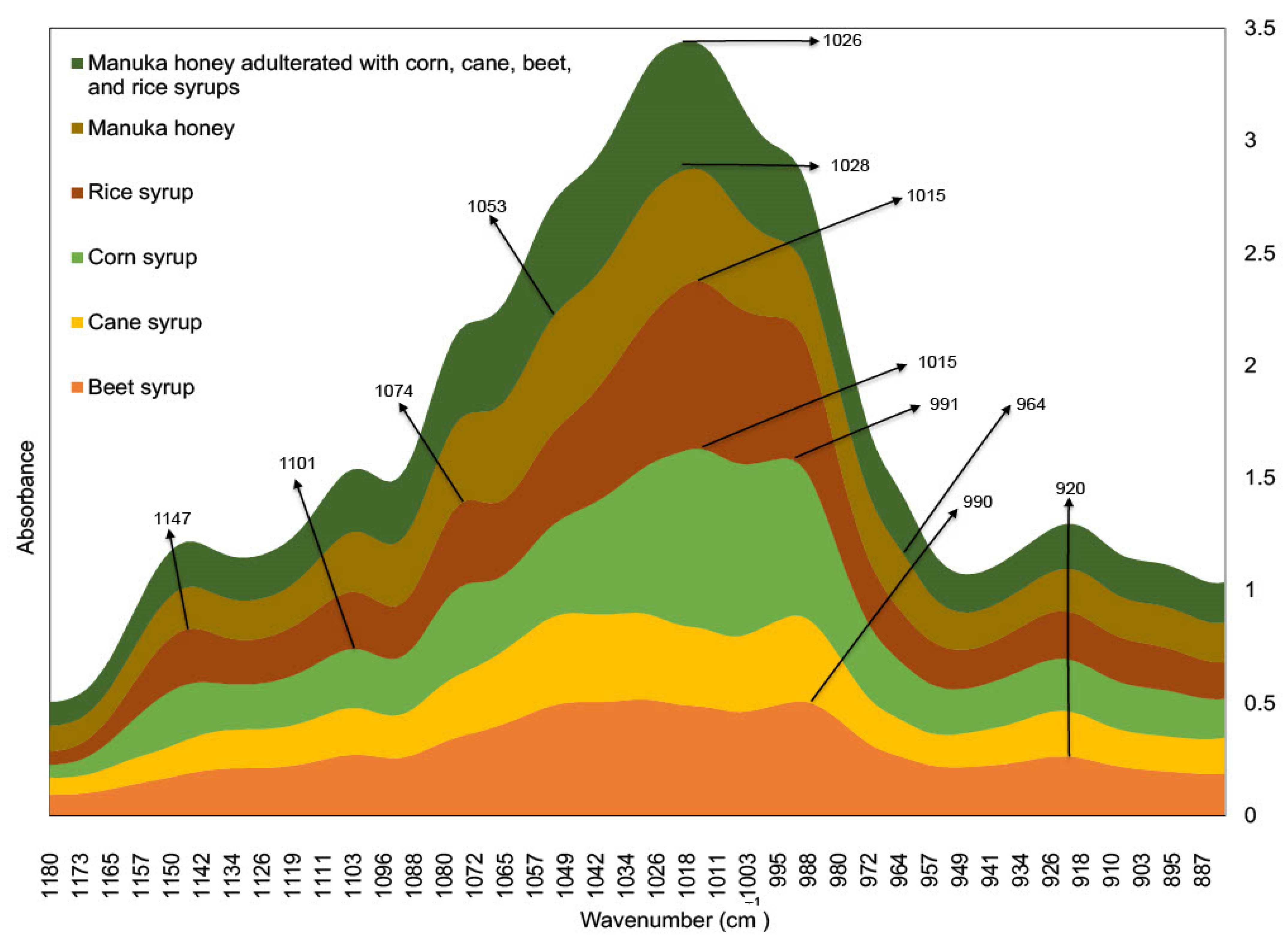
3.2. Analysis of the Specific Spectral Region (1501–799 cm⁻¹)

We compared the results obtained above with those obtained by performing signal preprocessing and PLS analysis of selected spectral regions (1501–799 cm⁻¹) harboring the spectral regions of interest present in the syrup adulterants. The RMSECV results garnered comparable values among the different signal processing techniques (Table 1). Therefore, when choosing the best model, we examined the results and compared the RMSECV to the RMSEP values (Table 1 and Table 2). In a comparison of the RMSECV (Table 1) and RMSEP (Table 2) values, in addition to the R²values (Table 3), using various signal processing techniques across the specific spectral region (1501–799 cm⁻¹), the first derivative test garnered optimum results $({\mathrm{RMSECV}}_{\mathrm{average}}=0.021,{ \mathrm{RMSEP}}_{\mathrm{average}}=0.014,{ \mathrm{R}}_{\mathrm{average}}^2=0.859)$ (Table 1, Table 2 and Table 3). The average values across the four adulterant syrups from the RMSECV (0.021) to the RMSEP (0.014) has decreased, and the R²value (0.859) indicates a good fit between the measured and predicted values ($\%\frac{\mathrm{w}}{\mathrm{w}})$ for the respective syrup adulterants (Table 1, Table 2 and Table 3).

The determination of which region garnered the best result was made by comparison of all results obtained using various signal preprocessing techniques (Table 1, Table 2 and Table 3). Optimum results were achieved by setting a specific spectral region for various preprocessing techniques (Table 1, Table 2 and Table 3). Various preprocessing techniques, including second derivative, moving average, binning, Savitzky–Golay, and SNV, as applied to the specific spectral region (1501–799 cm⁻¹) improved the results for most RMSECV, RMSEP, and R² parameters across the four syrup adulterants with the first derivative technique garnering the most optimum results (${\mathrm{RMSECV}}_{\mathrm{average}}=0.021,{ \mathrm{RMSEP}}_{\mathrm{average}}=0.014,{ \mathrm{R}}_{\mathrm{average}}^2=0.859)$ (Table 1, Table 2 and Table 3).

Using first derivative signal processing technique, close examination of the RMSECV as a function of the number of components showa that four, four, five, and four components are sufficient to have low errors of cross-validation (i.e., RMSECV) in the calibration set for the syrup adulterants of corn, cane, beet, and rice, respectively (Figure 4).

Using the first derivative signal processing techniques and the aforementioned numbers of components (Figure 4), the results of our study show that a good linearity is obtained between the predicted and measured concentrations ($\%\frac{\mathrm{w}}{\mathrm{w}}$) of adulterants in the training and testing sets (Figure 5).

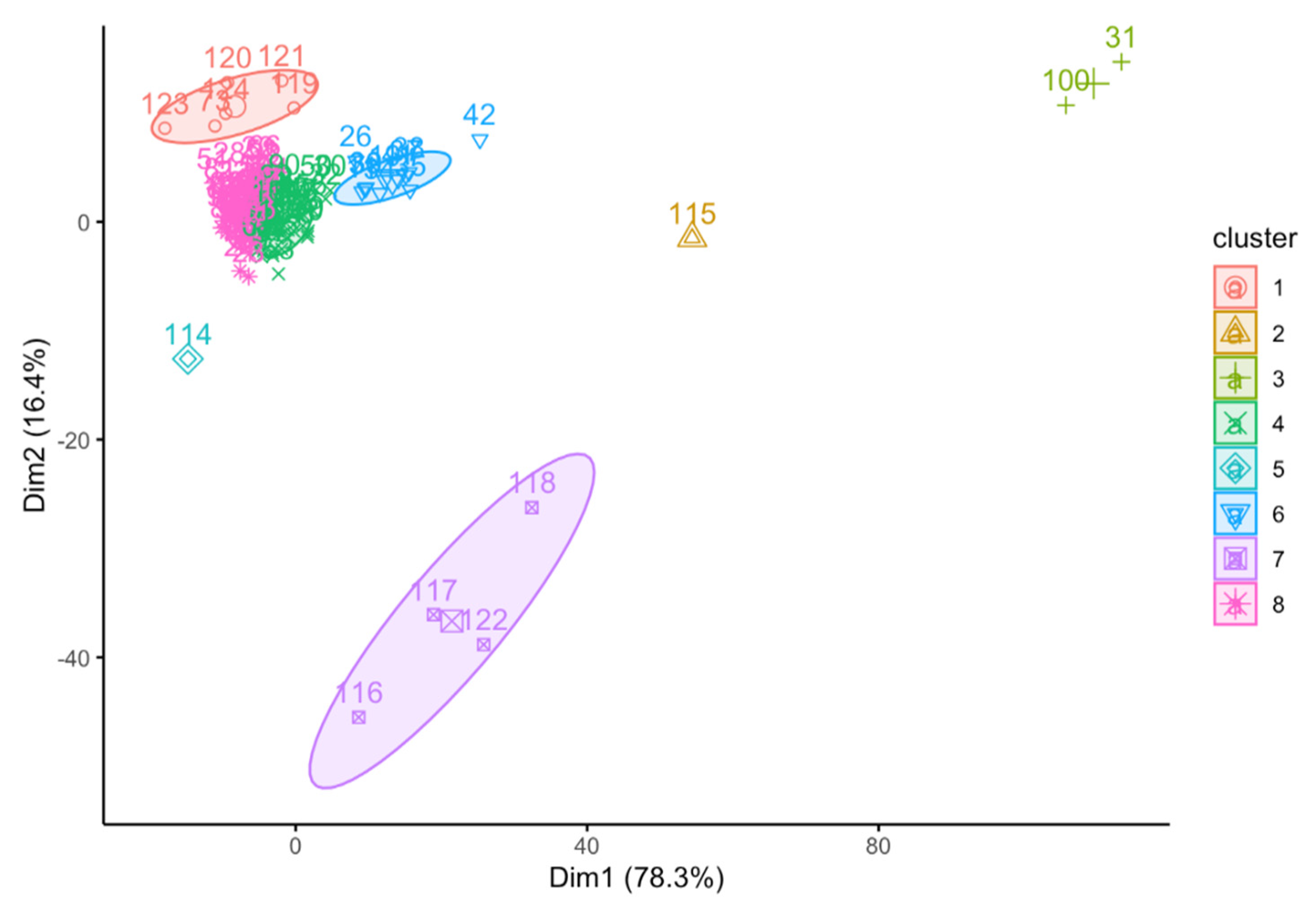
3.3. Exploratory Analysis of Syrup Adulterants and Honey Samples

In an attempt to determine any pattern formed among our adulterated honey samples (i.e., calibration and testing sets), pure honey samples (i.e., Standard Manuka honey), as well as selected adulterants, we performed PCA and cluster analysis using absorbance data points from a specific spectral region (1501–799 cm⁻¹) harboring sugars of interest (i.e., glucose, fructose, and sucrose; commonly found in syrups and honeys used in this study) (Figure 6). Our analysis was able to discriminate samples according to the presence or absence of syrup adulterants. For example, cluster 1 (i.e., samples 119–121, 123–124) shows standard pure Manuka honey samples (i.e., unadulterated honey samples). Within cluster 1, there exists the presence of sample 73, a full factorial design training set sample consisting of only pure unadulterated Manuka honey (i.e., absence of any corn, cane, beet, and rice syrups) (Figure 6) (c.f. Table S3).

Cluster 7 (i.e., samples 116–118, 122) grouped samples belonging to pure syrup adulterants. Specifically, sample 116 is a pure corn syrup, samples 117 and 122 are pure rice syrups, while sample 118 is a pure cane syrup. Of note are samples 114 and 115, belonging to pure beet and another pure cane syrup. These samples are clearly out of any typical clustering and their ingredients may warrant further investigation to explain this outcome (Figure 6) (c.f. Table S3).

Cluster 6 shows samples containing very low amounts of any of the adulterants. Specifically, most of the samples within this cluster contain zero percent adulterant in either one to three of the component syrup adulterants. Cluster 4, on the other hand, shows samples containing also low amounts of the syrup adulterants. Generally, cluster 4 has a higher amount of corn syrup levels ($\%{\frac{\mathrm{w}}{\mathrm{w}}}_{\mathrm{corn} \mathrm{average}}=6.28\%)$ than cluster 6 ($\%{\frac{\mathrm{w}}{\mathrm{w}}}_{\mathrm{corn} \mathrm{average}}=3.41\%)$. Further, cluster 4 has also a higher amount of rice syrup levels ($\%{\frac{\mathrm{w}}{\mathrm{w}}}_{\mathrm{rice} \mathrm{average}}=9.99\%)$ than cluster 6 ($\%{\frac{\mathrm{w}}{\mathrm{w}}}_{\mathrm{rice} \mathrm{average}}=6.23\%)$. The levels of cane and beet syrups, on the other hand, are higher in cluster 6 ($\%{\frac{\mathrm{w}}{\mathrm{w}}}_{\mathrm{cane} \mathrm{average}}=9.36\%; \%{\frac{\mathrm{w}}{\mathrm{w}}}_{\mathrm{beet} \mathrm{average}}=6.11\%)$ than in cluster 4 ($\%{\frac{\mathrm{w}}{\mathrm{w}}}_{\mathrm{cane} \mathrm{average}}=5.37\%; \%{\frac{\mathrm{w}}{\mathrm{w}}}_{\mathrm{beet} \mathrm{average}}=3.60\%)$ (Figure 6) (c.f. Table S3). Per our PCA and cluster analyses of the specific spectral region, it can be concluded that those samples having similar properties were grouped together.

Comprehensive comparison and examination of the performance of various signal processing techniques using the entire spectral region (3996–650 cm⁻¹) and specific spectral region (1501–799 cm⁻¹) for the direct quantification of syrup adulterants in honey has never been explored in previous studies. Further, while previous studies were focused on the pattern recognition of honey syrup adulteration for one syrup (e.g., identification of rice adulterated honey vs. unadulterated honey), this study offers the advantage of simultaneously quantifying four syrup adulterants in honey using PLS, FTIR, and first derivative signal processing technique [42]. The first derivative signal processing technique garnered the most optimum results using the specific spectral region $({\mathrm{RMSECV}}_{\mathrm{average}}=0.021,{ \mathrm{RMSEP}}_{\mathrm{average}}=0.014,{ \mathrm{R}}_{\mathrm{average}}^2=0.859)$ across all syrup adulterants as mentioned earlier.

An exploratory analysis to assess the utility of this specific spectral region in the pattern recognition of samples based on their adulterant contents shows that this region is effective in discriminating samples according to the presence or absence of syrup adulterants. Results of this can be applied to determine the utility of the first derivative focused on the specific spectral region harboring the functional groups of interest for the direct determination of specific analytes.

4. Conclusions

ATR-FTIR in conjunction with chemometric PLS analysis has proven to be useful in the development of a quick and facile method of quantifying corn, cane, beet, and rice syrup concentrations in honey. Specific spectral region (1501–799 cm⁻¹) garnered optimal results, with lower RMSECV and RMSEP, while also having a higher R² value in comparison to the entire spectral region. A comparison of the RMSECV, RMSEP, and R² values of the specific spectral region revealed that first derivative signal processing yielded optimal results. Using the same region, a PCA analysis also allowed for the discrimination of various syrup adulterants, honey, and adulterated honeys. The study can provide a direction as to the utility of the aforementioned region and first derivative signal processing technique for both the quantitative and qualitative identification of syrup adulterants in honey.

References

1. Fakhlaei, R.; Selamat, J.; Khatib, A.; Razis, A.F.A.; Sukor, R.; Ahmad, S.; Babadi, A.A. The Toxic Impact of Honey Adulteration: A Review. Foods 2020, 9, 1538. [Google Scholar] [CrossRef] [PubMed]
2. Ciursă, P.; Pauliuc, D.; Dranca, F.; Ropciuc, S.; Oroian, M. Detection of Honey Adulterated with Agave, Corn, Inverted Sugar, Maple and Rice Syrups Using FTIR Analysis. Food Control 2021, 130, 108266. [Google Scholar] [CrossRef]
3. Kelly, J.F.D.; Downey, G.; Fouratier, V. Initial Study of Honey Adulteration by Sugar Solutions Using Midinfrared (MIR) Spectroscopy and Chemometrics. J. Agric. Food Chem. 2004, 52, 33–39. [Google Scholar] [CrossRef] [PubMed]
4. Sivakesava, S.; Irudayaraj, J. A Rapid Spectroscopic Technique for Determining Honey Adulteration with Corn Syrup. J. Food Sci. 2001, 66, 787–791. [Google Scholar] [CrossRef]
5. Siddiqui, A.J.; Musharraf, S.G.; Choudhary, M.I.; Rahman, A.-U. Application of Analytical Methods in Authentication and Adulteration of Honey. Food Chem. 2017, 217, 687–698. [Google Scholar] [CrossRef]
6. Ribeiro, R.D.O.R.; Mársico, E.T.; da Silva Carneiro, C.; Monteiro, M.L.G.; Júnior, C.C.; de Jesus, E.F.O. Detection of Honey Adulteration of High Fructose Corn Syrup by Low Field Nuclear Magnetic Resonance (LF 1H NMR). J. Food Eng. 2014, 135, 39–43. [Google Scholar] [CrossRef]
7. Ruiz-Matute, A.I.; Soria, A.C.; Martínez-Castro, I.; Sanz, M.L. A New Methodology Based on GC−MS To Detect Honey Adulteration with Commercial Syrups. J. Agric. Food Chem. 2007, 55, 7264–7269. [Google Scholar] [CrossRef]
8. Başar, B.; Özdemir, D. Determination of Honey Adulteration with Beet Sugar and Corn Syrup Using Infrared Spectroscopy and Genetic-Algorithm-Based Multivariate Calibration. J. Sci. Food Agric. 2018, 98, 5616–5624. [Google Scholar] [CrossRef]
9. Se, K.W.; Wahab, R.A.; Syed Yaacob, S.N.; Ghoshal, S.K. Detection Techniques for Adulterants in Honey: Challenges and Recent Trends. J. Food Compos. Anal. 2019, 80, 16–32. [Google Scholar] [CrossRef]
10. Mendes, E.; Duarte, N. Mid-Infrared Spectroscopy as a Valuable Tool to Tackle Food Analysis: A Literature Review on Coffee, Dairies, Honey, Olive Oil and Wine. Foods 2021, 10, 477. [Google Scholar] [CrossRef]
11. Cozzolino, D.; Corbella, E.; Smyth, H.E. Quality Control of Honey Using Infrared Spectroscopy: A Review. Appl. Spectrosc. Rev. 2011, 46, 523–538. [Google Scholar] [CrossRef]
12. Brereton, R.G. Introduction to Multivariate Calibration in Analytical Chemistry. Analyst 2000, 125, 2125–2154. [Google Scholar] [CrossRef]
13. Næs, T.; Isaksson, T.; Fearn, T.; Davies, T. A User-Friendly Guide to Multivariate Calibration and Classification; NIR Publications: Chichester, UK, 2002. [Google Scholar]
14. Groemping, U.; Amarov, B.; Xu, H. DoE.Base: Full Factorials, Orthogonal Arrays and Base Utilities for DoE Packages, R Package Version 1.2; 2021. Available online: https://www.r-project.org/ (accessed on 23 December 2022).
15. Lenth, R. Rsm: Response-Surface Analysis, R Package Version 2.10.3; 2021. Available online: https://www.r-project.org/ (accessed on 23 December 2022).
16. RStudio. Available online: https://rstudio.com/ (accessed on 20 September 2021).
17. Liland, K.H.; Mevik, B.-H.; Wehrens, R.; Hiemstra, P. Pls: Partial Least Squares and Principal Component Regression, R Package Version 2.8-0; 2021. Available online: https://www.r-project.org/ (accessed on 23 December 2022).
18. Arroz, E.; Jordan, M.; Dumancas, G.G. Development of a Direct Spectrophotometric and Chemometric Method for Determining Food Dye Concentrations. Appl. Spectrosc. 2017, 71, 1633–1639. [Google Scholar] [CrossRef] [PubMed]
19. Adams, L.J.; Bello, G.; Dumancas, G.G. Development and Application of a Genetic Algorithm for Variable Optimization and Predictive Modeling of Five-Year Mortality Using Questionnaire Data. Bioinforma. Biol. Insights 2015, 9s3, BBI.S29469. [Google Scholar] [CrossRef] [PubMed] [Green Version]
20. G Dumancas, G.; Bello, G.; Hughes, J.; Diss, M. Comparison of Chemometric Algorithms for Multicomponent Analyses and Signal Processing: An Example from 4-(2-Pyridylazo) Resorcinol-Metal Colored Complexes. Recent Pat. Signal Process. Discontin. 2014, 4, 106–115. [Google Scholar] [CrossRef]
21. Dumancas, G.G.; Ramasahayam, S.; Bello, G.; Hughes, J.; Kramer, R. Chemometric Regression Techniques as Emerging, Powerful Tools in Genetic Association Studies. TrAC Trends Anal. Chem. 2015, 74, 79–88. [Google Scholar] [CrossRef]
22. Otto, M. Chemometrics: Statistics and Computer Application in Analytical Chemistry; John Wiley & Sons: Hoboken, NJ, USA, 2016. [Google Scholar]
23. Brereton, R.G. Chemometrics: Data Driven Extraction for Science; John Wiley & Sons: Hoboken, NJ, USA, 2018. [Google Scholar]
24. Stevens, A.; Ramirez-Lopez, L. Prospectr: Miscellaneous Functions for Processing and Sample Selection of Vis-NIR Diffuse Reflectance Data, R Package Version 0.1.3; 2014. Available online: https://www.r-project.org/ (accessed on 23 December 2022).
25. Zimmermann, B.; Kohler, A. Optimizing Savitzky–Golay Parameters for Improving Spectral Resolution and Quantification in Infrared Spectroscopy. Appl. Spectrosc. 2013, 67, 892–902. [Google Scholar] [CrossRef] [Green Version]
26. Stevens, A.; Ramirez-Lopez, L.; Hans, G. Prospectr: Miscellaneous Functions for Processing and Sample Selection of Spectroscopic Data, R Package Version 0.2.2; 2021. Available online: https://www.r-project.org/ (accessed on 23 December 2022).
27. Savitzky, A.; Golay, M.J. Smoothing and Differentiation of Data by Simplified Least Squares Procedures. Anal. Chem. 1964, 36, 1627–1639. [Google Scholar] [CrossRef]
28. Wickham, H. Ggplot2: Elegant Graphics for Data Analysis; Use R! Springer: New York, NY, USA, 2009; ISBN 978-0-387-98141-3. [Google Scholar]
29. Han, J.; Kamber, M.; Pei, J. Data Mining, Southeast Asia Edition: Concepts and Techniques; Morgan Kaufmann: Burlington, MA, USA, 2006. [Google Scholar]
30. Chakrabarti, S.; Cox, E.; Frank, E.; Güting, R.H.; Han, J.; Jiang, X.; Kamber, M.; Lightstone, S.S.; Nadeau, T.P.; Neapolitan, R.E.; et al. Data Mining: Know It All; Morgan Kaufmann: Burlington, MA, USA, 2008; ISBN 978-0-08-087788-4. [Google Scholar]
31. Faber, N.K.M. Estimating the Uncertainty in Estimates of Root Mean Square Error of Prediction: Application to Determining the Size of an Adequate Test Set in Multivariate Calibration. Chemom. Intell. Lab. Syst. 1999, 49, 79–89. [Google Scholar] [CrossRef]
32. Kassambara, A.; Mundt, F. Factoextra: Extract and Visualize the Results of Multivariate Data Analyses, R Package Version 1.0.5; 2017. Available online: https://www.r-project.org/ (accessed on 23 December 2022).
33. Timm, N.H. Applied Multivariate Analysis: Springer Texts in Statistics; Springer: New York, NY, USA, 2002. [Google Scholar]
34. Ferreiro-González, M.; Espada-Bellido, E.; Guillén-Cueto, L.; Palma, M.; Barroso, C.G.; Barbero, G.F. Rapid Quantification of Honey Adulteration by Visible-near Infrared Spectroscopy Combined with Chemometrics. Talanta 2018, 188, 288–292. [Google Scholar] [CrossRef]
35. Callao, M.P.; Ruisánchez, I. An Overview of Multivariate Qualitative Methods for Food Fraud Detection. Food Control 2018, 86, 283–293. [Google Scholar] [CrossRef]
36. Spink, J.; Moyer, D.C.; Speier-Pero, C. Introducing the Food Fraud Initial Screening Model (FFIS). Food Control 2016, 69, 306–314. [Google Scholar] [CrossRef]
37. Head, J.; Kinyanjui, J.; Talbott, M. FTIR-ATR Characterization of Commercial Honey Samples and Their Adulteration with Sugar Syrups Using Chemometric Analysis. Pittcon 2015, 2220–2221. [Google Scholar]
38. Lang, J.; McNitt, L. The Use of FT-IR Spectroscopy as a Technique for Verifying Maple Syrup Authenticity; PerkinElmer, Inc.: Shelton, CT, USA, 2014. [Google Scholar]
39. Tul’chinsky, V.M.; Zurabyan, S.E.; Asankozhoev, K.A.; Kogan, G.A.; Khorlin, A.Y. Study of the Infrared Spectra of Oligosaccharides in the Region 1,000-40 Cm−1. Carbohydr. Res. 1976, 51, 1–8. [Google Scholar] [CrossRef]
40. Hineno, M. Infrared Spectra and Normal Vibration of β-d-Glucopyranose. Carbohydr. Res. 1977, 56, 219–227. [Google Scholar] [CrossRef]
41. Smith, B.C. Alcohols—The Rest of the Story. Spectroscopy 2017, 32, 19–23. [Google Scholar]
42. Li, Q.; Zeng, J.; Lin, L.; Zhang, J.; Zhu, J.; Yao, L.; Wang, S.; Yao, Z.; Wu, Z. Low Risk of Category Misdiagnosis of Rice Syrup Adulteration in Three Botanical Origin Honey by ATR-FTIR and General Model. Food Chem. 2020, 332, 127356. [Google Scholar] [CrossRef]
Figure 1. Vector normalized Fourier transform infrared spectra of the training set.
Chemosensors 10 00051 g001
Figure 2. Vector normalized Fourier transform infrared spectra of the testing set.
Chemosensors 10 00051 g002
Figure 3. Fourier transform infrared spectra of syrup adulterants (i.e., corn, cane, beet, and rice), standard Manuka honey, and standard Manuka honey adulterated with corn, cane, beet, and rice syrups.
Chemosensors 10 00051 g003
Figure 4. Root mean square error of cross validation (RMSECV) as a function of the number of components for different syrups. (a) RMSECV as a function of the number of components for corn with 4 factors chosen, (b) RMSECV as a function of the number of components for cane with 4 factors selected, (c) RMSECV as a function of the number of components for beet with 5 factors selected, (d) RMSECV as a function of the number of components for rice with 4 factors chosen.
Chemosensors 10 00051 g004
Figure 5. (a) Predicted vs. measured corn syrup (% w/w) using the first derivative signal processing technique in the specific spectral region for both the training and test sets (R2 = 0.8529), (b) Predicted vs. measured cane syrup (% w/w) using the first derivative signal processing technique in the specific spectral region for both the training and test sets (R2 = 0.7716), (c) Predicted vs. measured beet syrup (% w/w) using the first derivative signal processing technique in the specific spectral region for both the training and test sets (R2 = 0.8646), (d) Predicted vs. measured rice syrup (% w/w) using the first derivative signal processing technique in the specific spectral region for both the training and test sets (R2 = 0.9437).
Chemosensors 10 00051 g005
Figure 6. Principal component analysis of syrup adulterants and honey samples.
Chemosensors 10 00051 g006