Convolutional Neural Network Applications in Fire Debris Classification

Abstract

Convolutional neural networks (CNNs) are inspired by the visual cortex of the brain. In this work, CNNs, are applied to classify ground truth samples as positive or negative for ignitable liquid residue (ILR+ and ILR−, respectively). Known ground truth samples included laboratory-generated fire debris samples, neat ignitable liquids (ILs), single-substrate (SUB) burned samples and computationally generated (in silico) training samples. The images were generated from the total ion spectra for both training and test datasets by applying a wavelet transformation. The training set consisted of 50,000 in silico-generated fire debris samples. The probabilities generated from the CNN are used to calculate the likelihood ratios. These likelihood ratios were calibrated using logistic regression and the empirical cross-entropy (ECE) plots were used to investigate the calibration of the probabilities of the presence of ILRs (i.e., probability of belonging to class ILR+). The performance of the model was evaluated by the area under the receiver operating characteristic plots (ROC AUC). The ROC AUC for the laboratory-generated fire debris samples and the combined IL and SUB samples was 0.87 and 0.99, respectively. The CNNs trained on in silico data did significantly better predicting the classification of the pure IL (ILR+) and SUB (ILR−) samples. Nonetheless, the classification performance for laboratory-generated samples was sufficient to aid forensic analysts in the classification of casework samples.

1. Introduction

Fire debris analysis involves the search for traces of ignitable liquid residue in samples collected from a fire scene. The presence of ignitable liquid residue can be an indication that a substance was added to aid in starting the fire. Fire debris samples are analyzed by gas chromatography–mass spectrometry, the “gold standard” for these analyses. The total ion chromatograms (TICs), the extracted ion profiles (EIPs) for alkane, alkene, alcohol, aromatic, cycloalkane, ester, ketone and polynuclear aromatic compounds [1,2], the identification of individual compounds, and visual pattern recognition are utilized to determine whether the sample is positive or negative for ignitable liquid residues (ILRs). Data analysis and interpretation are performed following the standard method described in ASTM E1618-01 [3]. Under this protocol, reporting guidelines require that a sample be designated as positive or negative for ILRs and the protocol does not allow for assigning a strength or evidential value to the sample. According to ASTM E1618, ignitable liquids are classified into eight main classes based on their major organic compound profiles, processing (distillates) and product use (gasoline) [3]. These classes are gasoline (GAS), petroleum distillates (PDs), isoparaffinic (ISO), aromatic (AR), naphthenic paraffinic (NP), normal alkane (nA), oxygenates (OXYs) and miscellaneous (MISC) [3]. The designation of multiple classes of liquid helps the analyst to organize their data analysis strategy and can help the investigator in identifying products from each class. The final decision of whether the sample contains ILRs or not is subjectively based on the individual analyst’s interpretation of the data with a case review by a second analyst or supervisor being common. If the original analysis or review does not introduce the guardrails of linear sequential unmasking or related protocols, the chances of bias being introduced into the process are increased [4,5,6,7]. Studies have been performed in presenting the presence or absence of ILRs as a likelihood ratio that has been calculated objectively by machine learning methods [8,9,10,11,12,13]. The work reported here presents another likelihood ratio calculation method that uses probabilities generated by convolutional neural networks.

Convolutional neural networks (CNNs) are a type of deep learning artificial neural network (ANN) with convolutional feature extraction layers and multiple fully connected layers. The CNN essentially learns to identify the features in a set of images that are important for classifying the images into specific categories. The human brain inspires both the less complicated ANN and CNN architectures, but specifically, the CNN is inspired by the visual cortex of the human brain [14]. Deep learning is a subsection of machine learning that can train a computer to perform human-like tasks, such as speech recognition, image recognition, etc.

Deep learning is finding use as an assistant or partner to technicians in medical image analysis [15,16,17], genomics [18,19,20] and dentistry [21,22,23]. In forensic science applications, deep learning is used in facial recognition [24], exploring dental records [25] and cyber security [26]. The purpose of this work is to apply convolutional neural networks for fire debris classification. In this study, the model was used to calculate the probability of the presence of ILRs in test samples.

CNNs consist of three types of layers: convolutional, pooling and fully connected (or dense) layers. The output of this network is a probability of the sample to belong to a specific class. In this work, the CNN provides the probability that a sample contains ILRs and, therefore, belongs to the class ILR+ with a probability P(ILR+|E), or that ILRs are absent, and the sample belongs to the class ILR− with a probability P(ILR−|E). These two posterior probabilities are conditioned on the evidence E. The two posterior probabilities must sum to a value of 1, as the two classes are exclusive and comprehensive (i.e., a sample may contain ILRs or not, there is no alternative classification). The likelihood ratio is calculated from the odds form of Bayes’ theorem, Equation (1), and a knowledge of the prior odds. The likelihood ratio is the ratio of the probabilities of observing the evidence under the two hypotheses of class membership: P(E|ILR+)/P(E|ILR−). The prior odds, P(ILR+)/P(ILR−), are taken to be equal to the ratio of probabilities of samples in the machine learning training set belonging to class ILR+ or ILR−. These are probabilities that we control when the training set is generated. When the prior odds are equal to 1, the posterior odds are equal to the likelihood ratio, Equation (1). All the programming for this work was performed using kerasR [27] and tensorflow [28].

$$\frac{P\left(ILR+|E\right)}{P\left(ILR-|E\right)}=\frac{P\left(E|ILR+\right)}{P\left(E|ILR-\right)}\times \frac{P\left(ILR+\right)}{P\left(ILR-\right)}$$

(1)

In the neural network, the first layer is the input layer, which carries the input image’s dimension (number of pixels and channels). The main building blocks of the network are the convolutional layers which contain kernels that spread entirely through the input that generates an activation map [29,30]. These convolutional layers are followed by pooling layers. In addition, a rectified linear unit activation (ReLU) was applied in convolutional layers to increase the nonlinearity of the network, Equation (2).

$$f\left(x\right)=\{\begin{array}{c}0\\ x\end{array} \begin{array}{c}for x\le 0\\ for x>0 \end{array}=\max \left\{0,x\right\}$$

(2)

When the ReLU function is applied, if value x > 0 it will return x, whereas if x ≤ 0, then it will return 0. Detailed information about the network used in this work will be discussed in the Materials and Methods section.

In the convolution process, the kernel (or filter) overlaps the image to compute the product between the numbers at each location in the kernel and the corresponding location within the overlapped portion of the input image. The sum of these products generates the output of this process, and the output is assigned to the image cell corresponding to the location of the central unit in the filter. The filter is then shifted by one pixel/unit to the right. When the filter reaches the end of the row of pixels, it returns to the left side of the image and drops down one pixel. The kernel starts on the top left corner of the image, and the process is continued until the kernel reaches the bottom right corner of the input image [31]. This computation is repeated for each kernel in the convolutional layer, followed by ReLu activation.

The pooling layers reduce the dimensionality of the image and the complexity of the computational model by downsampling the feature maps. In the model used in this work, max-pooling was applied after each convolutional layer. In max-pooling, the maximum value in each section from the convolution output is selected based on the size of the pooling matrix. The selected unit’s value is then placed in the corresponding pixel of the pooling output. In this work, the size of the pooling matrix was 2 × 2. The single largest value is selected and placed in a cell in the pooling output. Therefore, the entries from a 2 × 2 set of cells are replaced by a single cell and this process reduces the dimension of the convolution layer output by half.

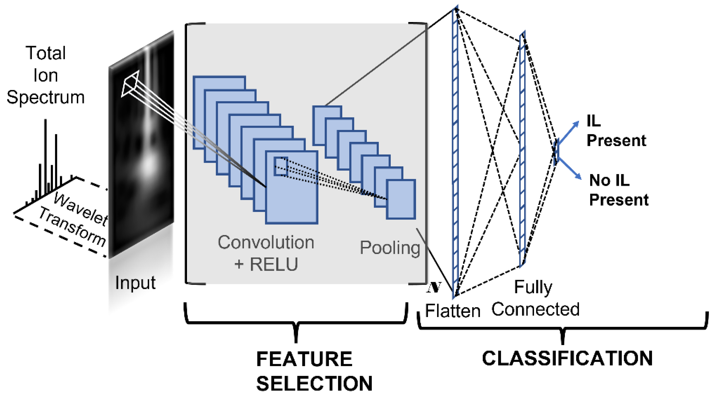
The convolution and pooling were followed by layer flattening, where the final output matrix from the convolution and subsequent pooling was unfolded into a single column. This output is then fed into a set of fully connected layers analogous to those found in a simple artificial neural network. When the final pooling layer is flattened, the output corresponds to a set of features that feed into the fully connected portion of the network. The combined convolution and pooling layers perform feature selection. The fully connected layers contain neurons that provide the final result from the model. Dropout layers are included between the fully connected layers to prevent the overfitting of the model.

The final dense layer of the network uses softmax activation, which generates the posterior probabilities. The softmax function operates on the input vector to produce an output vector of real numbers that sum to 1, which is provided in Equation (3) [32].

$$\sigma {\left(\overrightarrow{z}\right)}_i=\frac{e^{z_i}}{{{\displaystyle \sum }}_{j=1}^K{e}^{z_j}}$$

(3)

The term $\overrightarrow{z }$ is the input vector of the softmax function and z_i is the element in the input vector, whereas $e^{z_i}$ is the exponential of z_i. The symbol K is the number of classes in the problem; in this case, 2. The normalization factor is given by ${\displaystyle \sum }_{j=1}^K{e}^{z_j}$. The softmax function calculates the posterior probabilities of the samples that determine the classification. In this work, these posterior probabilities were used to assess if the sample belongs to class ILR+ or ILR−.

2. Materials and Methods

Three separate datasets were used for training and testing. A total of 50,000 in silico fire debris samples were generated as the training dataset. This dataset was generated using the samples in the Ignitable Liquid Reference Collection (ILRC) [33] and the Substrate [34] Database from the National Center for Forensic Science. The training set contained 25,000 ILSUB mixture samples (class ILR+) and 25,000 SUB mixture samples (class ILR−). One testing set, referred to as ILSUB, included samples of 1050 neat ignitable liquids in the ILRC (class ILR+) and 553 single-substrate samples from the Substrate Database (class ILR−). The second testing dataset, referred to as GTFD, was composed of laboratory-generated ground truth fire debris with 573 samples containing ignitable liquid residues (class ILR+), and 345 samples composed of mixtures of substrates and no added ignitable liquid (class ILR−) [13]. Laboratory-generated fire debris and in silico fire debris sample generation procedures were previously reported [13]. The ASTM IL class distribution of in silico training and the ILSUB and GTFD testing datasets are given in

Table 1. IL class population and distribution fractional contribution in parenthesis for the training and testing datasets.

Class	Class Population and Fractional Contribution: In Silico		Class Population and Fractional Contribution: GTFD		Class Population and Fractional Contribution: ILSUB
SUB	25,000	0.5	345	0.376	553	0.345
ISO	3125	0.0625	62	0.068	84	0.052
OXY	3125	0.0625	55	0.060	171	0.107
MISC	3125	0.0625	68	0.074	194	0.121
AL	3125	0.0625	60	0.065	60	0.037
GAS	3125	0.0625	65	0.071	83	0.052
PD	3125	0.0625	146	0.159	329	0.205
AR	3125	0.0625	59	0.064	72	0.045
NP	3125	0.0625	58	0.063	57	0.036
Total	50,000		918		1603

. When generating in silico data, the IL/SUB ratio in the in silico data distribution was made similar to the laboratory-generated fire debris samples. The distribution of the base 10 logarithm of IL/SUB ratios of ILR+ class samples from both in silico and GTFD are presented in Figure 1.

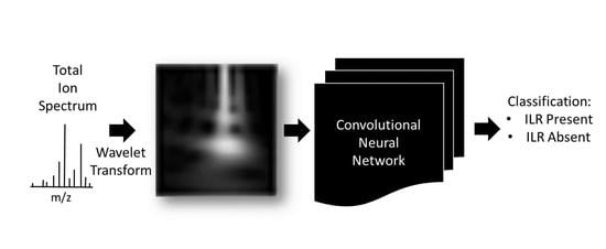
The TIS from the database and in silico samples were converted to images by wavelet transform [35]. The transform was performed using a Morlet wavelet applied to the TISs, which are treated as time series. The Morlet wavelet basis function is given by Equation (4), where $\eta$ is a nondimensional “time” parameter corresponding to the m/z in the TIS spectra and ${\omega }_0$ is a nondimensional frequency. Following an analogous approach to Torrence et al. [35], each TIS is treated as a time series $x_n$ of points evenly separated by $\delta t$ where $n=0\dots N-1$, and $N$ is the total number of values in the series. The TISs are composed of 129 values, separated by 1 m/z. The continuous wavelet transform for the series of $x_n$ points is given by their convolution with a scaled and translated ${\mathsf{\Psi }}_o\left(\eta \right)$, as given in Equation (5). In Equation (5), $s$ is the wavelet scale and the asterisk (*) indicates the complex conjugate. The scales for the calculations were the default power 2 scales constructed by the wavScalogram software [36]. The 260 values of $s_j$ were calculated based on Equations (6) and (7), where $s_0$ is the smallest resolvable scale and $J$ determines the largest scale. The scales were calculated as a sequence from $s_0=1.936027$ to $s_J=45$. A smaller $s_j$ corresponds to a more “compressed” wavelet (i.e., more compressed along the m/z axis of the TIS).

$${\mathsf{\Psi }}_o\left(\eta \right)={\pi }^{-1/4}{e}^{i{\omega }_0\eta }{e}^{-{\eta }^2/2}$$

(4)

$$W_n\left(s\right)={\left(\frac{\delta t}{s}\right)}^{1/2}{\displaystyle \sum }_{n^{\prime }=0}^{N-1}{x}_{n^{\prime }}{\mathsf{\Psi }}_0^{*}\left[\frac{\left(n^{\prime }-n\right)\delta t}{s}\right]$$

(5)

$$s_j=s_0{2}^{j\delta j}, j=0,1,\dots ,J$$

(6)

$$J=\delta j^{-1}lo{g}_2\left(N\delta t/s_0\right)$$

(7)

Figure 2 shows the total ion spectrum for a gasoline sample (a) and the corresponding “scalogram” (b) that was calculated using Equations (4)–(7). The shaded areas along the sides and bottom of the scalogram indicate the areas where edge effects come into play in the convolution. The abscissa scale for the TIS corresponds to the m/z values. The abscissa scale in the scalogram is labeled as xlim, which has a 1:1 correspondence with m/z; however, it is zero-based. At the smaller scales (top of the scalogram), the more compressed wavelet is acting as a filter and picking out the more intense peaks and local clusters of peaks in the TIS. As the scale increases, resulting in a less compressed wavelet, the higher intensity in the scalogram begins to correspond to the lower frequency patterns in the TIS. The resulting stacked set of wavelet power spectra, the scalogram, (Figure 2b) is presented as a false color image where the color represents the wavelet intensity. The scalograms were converted into a 50 × 50 grayscale image (Figure 2c, bottom panel) by sampling a 50 × 50 grid of points in proportion to the original dimensions of the scalogram. The intensity patterns in the grayscale images correspond to intensity changes occurring at different frequencies in the TIS. The 50 × 50 grayscale images were used for training the CNN.

The neural network used in this work consists of three convolutional layers, two max-pooling layers and a fully connected layer. Two dropout layers were added to prevent the overfitting of the model. These dropout layers randomly remove a portion of the total weights. In this instance, 50% of the weights were removed in each dropout layer randomly. The model was trained ten times and the average training and testing accuracies were calculated. The structure of the model applied in this work is presented in Figure 3.

The total number of parameters in this network was 2,711,490. In this model, 150 epochs were used to train the model fully and the batch size and cross-validation split were 500 and 0.2, respectively. For example, one epoch consists of 100 folds based on the batch number and in each fold, 20% of the samples were randomly selected from a batch of 500 samples for cross-validation. Finally, at the end of each epoch, the total validation and training accuracy for the model were calculated.

The plot of training and validation accuracies and losses for the 10th model is presented in Figure 4. The training and cross-validation accuracies of the model gradually increased through the number of epochs and remained constant at 0.94 and the loss gradually decreased and remained between 0.4 and 0.5. The loss for the cross-validation was not as high as the loss for the training set; however, the accuracy of the prediction for cross-validation closely paralleled the accuracy for the training set.

3. Results

3.1. Generated Images for ILRC and Fire Debris Data

Examples of a TIS and the corresponding scalogram and grayscale image are shown in Figure 2. The top panel shows the TIS for a gasoline sample. The most intense peaks in the TIS correspond to m/z 91 and 105, which result from the fragmentation of aromatic compounds in the sample. A set of less intense peaks can be seen around m/z 43 and 57. These peaks result from the fragmentation of aliphatic compounds in the sample. The middle panel shows the wavelet power spectrum. The smallest scales (top of the scalogram) correspond to the most compressed wavelets, which upon convolution with the TIS, give the largest coefficients (intensity) at xlim values corresponding to the areas of m/z 91, 105, 43 and 57. As the scale increases and the wavelet becomes less compressed, other areas of TIS intensity appearing at lower frequencies can be observed. For example, at a scale of approximately 15, two areas of intensity can be observed, one occurring in the lower m/z range where the aliphatic-derived ions appear and the second at a higher m/z range where the aromatic-derived ions appear. This example demonstrates how the wavelet transform highlights different intensity and frequency patterns in the TIS. Computer memory requirements limited the size of each image that could be used in training the convolutional neural network. To accommodate the memory limitations, each scalogram was reduced to a 50 × 50 grayscale image, as shown in the bottom panel in Figure 2. The scalogram reduction was accomplished by sampling from the wavScalogram-generated scalogram rows and columns corresponding to the ratio of input/output dimensions.

Additional images generated as examples from each neat IL class are shown in Figure 5 and have distinguishable features related to the corresponding TIS, as described in the previous paragraph. Some images generated from the substrate samples (MRN 1: cotton cloth, 33: hardwood, 63: olefin/nylon blend carpet) are also provided in Figure 5i–k. The images corresponding to samples from the Substrate Database (class ILR−) appear, in general, to have more complex structural features than the pure IL samples from different ASTM classes. Due to the complex chemical nature of the pyrolysis products, it is not possible to visibly select the features useful in leading to the correct classification of a sample as ILR+ or ILR−. The point of this work is to test if a convolutional neural network model can accomplish this task.

In images of GTFD samples from class ILR+, the pattern attributable to the IL becomes less obvious as the IL/SUB ratio decreases. This is demonstrated in Figure 6 for a sample containing ILRs from the ASTM AR solvent class and the substrate pyrolysis (see Figure 5a for IL scalogram). As the IL/SUB ratio decreases, the signal from the IL becomes weaker.

3.2. Likelihood Ratio Calculations

The average training accuracy from the cross-validation based on in silico data for the 10 models was 0.939 ± 0.003 and the average testing validation accuracies of GTFD and ILSUB across the same 10 models were 0.788 ± 0.011 and 0.988 ± 0.002, respectively. The accuracies are based on the ILR+ class assignment if the CNN posterior probability of ILR+ membership was greater than or equal to 0.5. The training and testing accuracies of the ten models are presented in

Table 2. Training and testing accuracies of the ten CNN models.

		Testing Accuracy
Model	Training Accuracy	ILSUB	FDIL
1	0.943	0.986	0.775
2	0.940	0.986	0.798
3	0.942	0.990	0.797
4	0.932	0.984	0.776
5	0.939	0.989	0.786
6	0.941	0.986	0.783
7	0.938	0.988	0.775
8	0.941	0.988	0.790
9	0.938	0.989	0.800
10	0.940	0.991	0.801

. The log base 10 likelihood ratios for the test data were calculated using the posterior probabilities provided by the CNN using the rearranged odds form of the Bayes equation, Equation (8).

$$\mathrm{LLR}=lo{g}_{10}\left(\frac{P(ILR+|E)}{P(ILR-|E)}\times \frac{P\left(ILR-\right)}{P\left(ILR+\right)}\right)$$

(8)

The probabilities generated from model 10 were selected for further calculations based on the testing accuracies for GTFD and ILSUB datasets. In this case, to calculate likelihood ratios, the prior odds were set to 1 since the number of samples belonging to the ILR+ and ILR− classes in the training model are equal. These uncalibrated LLRs were calibrated by logistic regression. Empirical cross-entropy (ECE) plots (Figure 7a,b) illustrate the LLR calibration for GTFD and ILSUB. The LLR following logistic regression calibration (solid red line) and the LLR resulting from pooled adjacent violator calibration (dashed blue line) indicate how well the posterior probabilities are calibrated [33]. The smaller the separation between these two lines, the better the logistic regression calibration. LLRs calculated by the posterior probabilities are used to generate receiver operating characteristic (ROC) curves to provide an evaluation of the performance of the model as a function of LLR decision thresholds. An ROC curve is defined by a plot between the true positive rate and false positive rate as a function of the decision threshold, and the area under the curve (AUC) serves as the performance metric for a classifier. The magnitude of calculated LLRs was not always directly proportional to the IL/SUB ratio in these GTFD samples containing ILRs (graphs not shown).

The average AUC for the 918 GTFD samples and 1603 ILSUB samples was 0.857 ± 0.007 (Figure 8a) and 0.993 ± 0.003 (Figure 8b), respectively. This indicates that the discrimination of neat ignitable liquids and single-substrate samples is higher than the substrate mixtures with and without ILRs.

Before reporting a categorical statement about the presence or absence of ILRs, the selection of a decision threshold is required [13]. This threshold value can be obtained by an iso-performance line with a defined slope which is tangent to the ROC convex hull (ROC CHULL) and maximizes the y-intercept. The optimal threshold is determined by where the iso-performance line intersects the ROC CHULL. The slope of the iso-performance line is determined by Equation (9) [37].

$$\frac{ T{P}_2-T{P}_1}{F{P}_2-F{P}_1}=\frac{p\left(n\right)c\left(p,n\right)}{p\left(p\right)c\left(n,p\right)}=m$$

(9)

In this equation,$\left(T{P}_2, F{P}_2\right)$ and $\left(T{P}_1, F{P}_1\right)$ are points in ROC space on the iso-performance line. The prior probabilities of positive and negative samples are given by $p\left(p\right)$ and $p\left(n\right)$, respectively. The costs of classifying a positive sample as negative can be given by $c(p,n$), whereas the costs of classifying a negative sample as positive are $c(n,p$). Since the prior odds are defined as 1 in the training dataset, the cost ratio is equal to the slope of the iso-performance line, which must be determined as acceptable by the laboratory. The ROC plots with iso-performance lines generated for ground truth fire debris data are presented in Figure 9. These plots were created from the LLRs that were calculated from the probabilities generated from model 10. The calculated optimal LLRs (decision thresholds) for slopes 10, 5 and 2.5 are 0.78, 0.78 and 0.22, respectively.

The sample classifications at LLRs 0.78 and 0.22 in GTFD are summarized in the confusion matrices provided in

Table 3. Confusion matrices for GTFD sample classifications at LLRs 0.78 and 0.22.

LLR = 0.78	Predicted class
Correct class	IL	SUB
IL	TP = 258 (45%)	FN = 315
SUB	FP = 9 (3%)	TN = 336
LLR = 0.22	Predicted class
Correct class	IL	SUB
IL	TP = 404 (71%)	FN = 169
SUB	FP = 38 (11%)	TN = 307

. In general, the true positive rate (correct classification as ILR+ in the presence of ILs) increased from 45% to 71% as the slope decreased; subsequently, the false positive rate (incorrect classification as ILR+ in the absence of ILRs) also increased from 3% to 11%.

The GTFD samples containing ILRs were further examined to identify the true positive and false positive rates of each ASTM E1618 IL class based on the optimal LLR decision threshold. TPR and FPR were calculated using Equations (10) and (11), given below. The results of these calculations are presented in

Table 4. True positive rates (TPRs) for each IL class for substrate mixtures (GTFD) containing ILRs and neat ILs from ILSUB data based on optimal decision threshold LLR values for slopes 10, 5 and 2.5.

IL Class	LLR = 0.78 (Slope = 10 and 5)	LLR = 0.22 (Slope = 2.5)
	TPR (%) (GTFD)	TPR (%) (GTFD)
AR	55.9	74.6
GAS	41.5	64.6
ISO	61.3	82.3
MISC	32.4	75
NAL	46.7	68.3
NP	56.9	74.1
OXY	21.8	45.5
PD	44.5	73.3

.

$$\mathrm{TPR}\%=\frac{\mathrm{Number}\mathrm{of}\mathrm{samples}\mathrm{where}\mathrm{LLR}>\mathrm{decision}\mathrm{threshold}\mathrm{in}\mathrm{each}\mathrm{class}}{\mathrm{Total}\mathrm{number}\mathrm{of}\mathrm{samples}\mathrm{in}\mathrm{each}\mathrm{class}}\times 100$$

(10)

$$\mathrm{FPR}\%=\frac{\mathrm{Number}\mathrm{of}\mathrm{samples}\mathrm{where}\mathrm{LLR}>\mathrm{decision}\mathrm{threshold}\mathrm{in}\mathrm{substrates}}{\mathrm{Total}\mathrm{number}\mathrm{of}\mathrm{substrate}\mathrm{samples}}\times 100$$

(11)

In the GTFD samples, LLRs ranged from 8.41 to −1.02 in the samples with ILRs. From this dataset, 474 samples had positive LLRs, and 99 samples had negative LLRs. In substrate mixture samples (those without ILRs), the LLRs ranged from 3.69 to −2.77.

The iso-performance lines were also created for the ROC curve generated for the ILSUB data using the LLRs calculated from the probabilities obtained from model 10 (Figure 10). In this, for slopes 10, 5 and 2.5, the TPR was 98%. The FPR and optimal LLR were 0.0% and −0.33, respectively. For these samples, changing the slope in the range of 2.5 to 10 did not affect the magnitude of the parameters.

The true positive rate (TPR) for neat ILs in the ILSUB data was also calculated using Equation (10) and are presented in

Table 5. True positive rates (TPRs) for each IL class for neat ILs from ILSUB data based on optimal decision threshold LLR values for slopes 10, 5 and 2.5.

IL Class	LLR = −0.33 (Slope = 10, 5 and 2.5)
	TPR (%) (ILSUB)
AR	100
GAS	100
ISO	100
MISC	94.3
NAL	100
NP	100
OXY	93
PD	99

.

In substrate mixtures from GTFD (those without ILRs), 84 samples had positive LLRs. Most of these substrate mixtures contained carpet (nylon, triexta or olefin), flooring (vinyl/linoleum or laminate), adhesive, roofing and plastic products. Although these samples do not contain ignitable liquid residues, the pyrolysis products may include chemicals typically present in some ASTM E1618 classes of ignitable liquid. For example, adhesives may contain compounds present in PD and AR liquids. Some vinyl materials pyrolyze to produce aromatic compounds.

The LLR range for the single-component ILSUB samples was 15.95 to −8.71, whereas the LLR range for the multi-component GTFD samples was only 8.41 to −2.77. The larger range of LLR values for ILSUB samples reflects a greater evidentiary value at the extremes. The compressed LLR range for the GTFD samples reflects the decrease in evidentiary value resulting from the mixture of ignitable liquid residue and multiple substrates. The larger ROC AUC for the ILSUB samples demonstrates a greater class separation than observed for the GTFD mixed samples.

4. Conclusions

Based on the AUC of ROC plots, it is evident that the application of CNNs trained on in silico samples works better for neat ILs and single-substrate samples (ILSUB) than the substrate mixtures with and without ILRs (GTFD). Although the ROC AUC for the GTFD samples was high (0.86), the TPRs (0.45 and 0.71) at the optimal operational points (0.78 and 0.22, respectively) are somewhat low for use in casework. An increase in the ROC AUC is required to overcome this challenge. Possible ways of achieving an increased ROC AUC include increasing the number of samples in the in silico training set by adding more variations of mixtures of substrates and ignitable liquids, varying the wavelet function, and further optimizing the CNN. In future work, the determination of epistemic uncertainty in the model will also be discussed to provide a more accurate depiction of the model estimations of sample classifications.

References

1. Keto, R.O.; Wineman, P.L. Detection of petroleum-based accelerants in fire debris by target compound gas chromatography/mass spectrometry. Anal. Chem. 1991, 63, 1964–1971. [Google Scholar] [CrossRef]
2. Keto, R.O. GC/MS Data Interpretation for Petroleum Distillate Identification in Contaminated Arson Debris. J. Forensic Sci. 1995, 40, 412–423. [Google Scholar] [CrossRef]
3. ASTM E 1618-01; Standard Test Method for Ignitable Liquid Residues in Extracts from Fire Debris Samples by Gas Chromatography—Mass Spectrometry. American Society for Testing and Materials: West Conshohocken, PA, USA, 2019.
4. Quigley-McBride, A.; Dror, I.E.; Roy, T.; Garrett, B.L.; Kukucka, J. A practical tool for information management in forensic decisions: Using Linear Sequential Unmasking-Expanded (LSU-E) in casework. Forensic Sci. Int. Synerg. 2022, 4, 100216. [Google Scholar] [CrossRef] [PubMed]
5. Curley, L.J.; Munro, J.; Dror, I.E. Cognitive and human factors in legal layperson decision making: Sources of bias in juror decision making. Med. Sci. Law 2022, 62, 206–215. [Google Scholar] [CrossRef]
6. Kukucka, J.; Dror, I. Human Factors in Forensic Science: Psychological Causes of Bias and Error; Oxford University Press: Oxford, UK, 2022. [Google Scholar]
7. Whitehead, F.A.; Williams, M.R.; Sigman, M.E. Decision theory and linear sequential unmasking in forensic fire debris analysis: A proposed workflow. Forensic Chem. 2022, 29, 100426. [Google Scholar] [CrossRef]
8. Waddell, E.E.; Song, E.T.; Rinke, C.N.; Williams, M.R.; Sigman, M. Progress Toward the Determination of Correct Classification Rates in Fire Debris Analysis. J. Forensic Sci. 2013, 58, 887–896. [Google Scholar] [CrossRef] [PubMed]
9. Waddell, E.E.; Williams, M.R.; Sigman, M.E. Progress Toward the Determination of Correct Classification Rates in Fire Debris Analysis II: Utilizing Soft Independent Modeling of Class Analogy (SIMCA). J. Forensic Sci. 2014, 59, 927–935. [Google Scholar] [CrossRef] [PubMed]
10. Sigman, M.E.; Williams, M.R. Assessing evidentiary value in fire debris analysis by chemometric and likelihood ratio approaches. Forensic Sci. Int. 2016, 264, 113–121. [Google Scholar] [CrossRef] [PubMed]
11. Allen, A.; Williams, M.R.; Thurn, N.A.; Sigman, M.E. Model Distribution Effects on Likelihood Ratios in Fire Debris Analysis. Separations 2018, 5, 44. [Google Scholar] [CrossRef]
12. Coulson, R.; Williams, M.R.; Allen, A.; Akmeemana, A.; Ni, L.; Sigman, M.E. Model-effects on likelihood ratios for fire debris analysis. Forensic Chem. 2018, 7, 38–46. [Google Scholar] [CrossRef]
13. Thurn, N.A.; Wood, T.; Williams, M.R.; Sigman, M.E. Classification of ground-truth fire debris samples using artificial neural networks. Forensic Chem. 2021, 23, 100313. [Google Scholar] [CrossRef]
14. Goodfellow, I.; Bengio, Y.; Courville, A. Deep Learning; MIT Press: Cambridge, MA, USA, 2016. [Google Scholar]
15. Sahiner, B.; Pezeshk, A.; Hadjiiski, L.M.; Wang, X.; Drukker, K.; Cha, K.H.; Summers, R.M.; Giger, M.L. Deep learning in medical imaging and radiation therapy. Med. Phys. 2019, 46, e1–e36. [Google Scholar] [CrossRef] [PubMed]
16. Suzuki, K. Overview of deep learning in medical imaging. Radiol. Phys. Technol. 2017, 10, 257–273. [Google Scholar] [CrossRef] [PubMed]
17. Kim, M.; Yun, J.; Cho, Y.; Shin, K.; Jang, R.; Bae, H.-J.; Kim, N. Deep learning in medical imaging. Neurospine 2019, 16, 657. [Google Scholar] [CrossRef] [PubMed]
18. Yue, T.; Wang, H. Deep learning for genomics: A concise overview. arXiv 2018, arXiv:1802.00810. [Google Scholar]
19. Zou, J.; Huss, M.; Abid, A.; Mohammadi, P.; Torkamani, A.; Telenti, A. A primer on deep learning in genomics. Nat. Genet. 2019, 51, 12–18. [Google Scholar] [CrossRef]
20. Kopp, W.; Monti, R.; Tamburrini, A.; Ohler, U.; Akalin, A. Deep learning for genomics using Janggu. Nat. Commun. 2020, 11, 3488. [Google Scholar] [CrossRef]
21. Hwang, J.-J.; Jung, Y.-H.; Cho, B.-H.; Heo, M.-S. An overview of deep learning in the field of dentistry. Imaging Sci. Dent. 2019, 49, 1–7. [Google Scholar] [CrossRef]
22. Rodrigues, J.A.; Krois, J.; Schwendicke, F. Demystifying artificial intelligence and deep learning in dentistry. Braz. Oral Res. 2021, 35. [Google Scholar] [CrossRef]
23. Corbella, S.; Srinivas, S.; Cabitza, F. Applications of deep learning in dentistry. Oral Surg. Oral Med. Oral Pathol. Oral Radiol. 2021, 132, 225–238. [Google Scholar] [CrossRef]
24. Zeng, J.; Zeng, J.; Qiu, X. Deep learning based forensic face verification in videos. In Proceedings of the 2017 International Conference on Progress in Informatics and Computing (Pic), Nanjing, China, 27–29 October 2017; IEEE: Nanjing, China, 2017; pp. 77–80. [Google Scholar]
25. Liang, Y.; Han, W.; Qiu, L.; Wu, C.; Shao, Y.; Wang, K.; He, L. Exploring Forensic Dental Identification with Deep Learning. Adv. Neural Inf. Process. Syst. 2021, 34, 3244–3258. [Google Scholar]
26. Karie, N.M.; Kebande, V.R.; Venter, H. Diverging deep learning cognitive computing techniques into cyber forensics. Forensic Sci. Int. Synerg. 2019, 1, 61–67. [Google Scholar] [CrossRef] [PubMed]
27. Allaire, J.J.; Chollet, F. keras: R Interface to ‘Keras’, R Package Version 2.9.0. 2021. Available online: https://cran.r-project.org/web/packages/keras/index.html (accessed on 20 September 2022).
28. Allaire, J.J.; Tang, Y. Tensorflow: R Interface to ‘TensorFlow’, R Package Version 2.9.0. 2021. Available online: https://cran.r-project.org/web/packages/tensorflow/index.html (accessed on 20 September 2022).
29. Ke, Q.; Liu, J.; Bennamoun, M.; An, S.; Sohel, F.; Boussaid, F. Chapter 5—Computer Vision for Human–Machine Interaction. In Computer Vision for Assistive Healthcare; Leo, M., Farinella, G.M., Eds.; Academic Press: Cambridge, MA, USA, 2018; pp. 127–145. [Google Scholar]
30. O’Shea, K.; Nash, R. An introduction to convolutional neural networks. arXiv 2015, arXiv:1511.08458. [Google Scholar]
31. Wu, J. Introduction to Convolutional Neural Networks; National Key Lab for Novel Software Technology, Nanjing University: Nanjing, China, 2017; Volume 5, p. 495. [Google Scholar]
32. Wood, T. What Is the Softmax Function? Available online: https://deepai.org/machine-learning-glossary-and-terms/softmax-layer (accessed on 3 April 2022).
33. Ignitable Liquid Reference Collection. National Center for Forensic Science. Available online: https://ilrc.ucf.edu/ (accessed on 3 May 2022).
34. Substrate Database. National Center for Forensic Science. Available online: https://ilrc.ucf.edu/substrate/index.php (accessed on 5 May 2022).
35. Torrence, C.; Compo, G.P. A practical guide to wavelet analysis. Bull. Am. Meteorol. Soc. 1998, 79, 61–78. [Google Scholar] [CrossRef]
36. Vicente, J.B.; Rafael, B. wavScalogram: Wavelet Scalogram Tools for Time Series Analysis. R Package Version 1.1.1. 2021. Available online: https://CRAN.R-project.org/package=wavScalogram (accessed on 20 September 2022).
37. Provost, F.; Fawcett, T. Robust Classification for Imprecise Environments. Mach. Learn. 2001, 42, 203–231. [Google Scholar] [CrossRef]
Figure 1. Log10 (IL/SUB) ratio of in silico and fire debris data.
Chemosensors 10 00377 g001
Figure 2. (a): total ion spectrum for a gasoline sample. (b): wavelet power spectrum for the TIS shown in the top panes. (c): grayscale image 50 × 50 created from the power spectrum shown in the middle panel.
Chemosensors 10 00377 g002
Figure 3. Schematic diagram of the CNN model used in this model (first dropout layer was added in between the third convolutional and first fully connected layer, and the second layer was added between two fully connected layers).
Chemosensors 10 00377 g003
Figure 4. Training and validation accuracies and loss of model 10 through 150 epochs.
Chemosensors 10 00377 g004
Figure 5. Images generated from representative TIS of each neat IL class: (a) AR, (b) GAS, (c) ISO, (d) MISC, (e) NA, (f) NP, (g) OXY, (h) PD and single substrates (i) MRN 1: cotton cloth, (j) MRN 33: hardwood, (k) MRN 63: olefin/nylon blend carpet.
Chemosensors 10 00377 g005
Figure 6. Images of fire debris samples containing aromatic (AR) ignitable liquid residue from the same liquid and the same substrate material mixture (cork plank vinyl flooring and ceiling tile), (a) IL/SUB = 1.37, (b) IL/SUB = 0.25.
Chemosensors 10 00377 g006
Figure 7. Empirical cross-entropy (ECE) plots generated for (a) GTFD and (b) ILSUB data for probabilities generated from model 10.
Chemosensors 10 00377 g007
Figure 8. (a) Receiver operating characteristic (ROC) plots for calibrated log-likelihood ratios calculated for GTFD data with and without ILRs; (b) ILSUB data (solid black curve indicates the average ROC curve for all 10 models, whereas the grey indicates the ROC curves from all 10 models).
Chemosensors 10 00377 g008
Figure 9. The change in TPR and FPR based on selected slopes (a) 10, (b) 5 and (c) 2.5 and the optimal operational LLRs (0.78, 0.78, 0.22) in the ROC plot generated for GTFD data with and without ILRs (solid gray line represents the ROC curve, whereas solid and dashed black curves represent ROC convex hull and generated iso-performance lines, respectively).
Chemosensors 10 00377 g009
Figure 10. The change in TPR and FPR based on selected slopes (a) 10, (b) 5 and (c) 2.5 and the optimal operational LLR is −0.33 in the ROC plot generated for ILSUB data (solid gray line represents the ROC curve, whereas solid and dashed black curves represent ROC convex hull and generated iso-performance lines, respectively).
Chemosensors 10 00377 g010