
Post-Analysis of Predictive Modeling with an Epidemiological Example

 , ,
, ,
Abstract
:1. Introduction
2. Materials and Methods
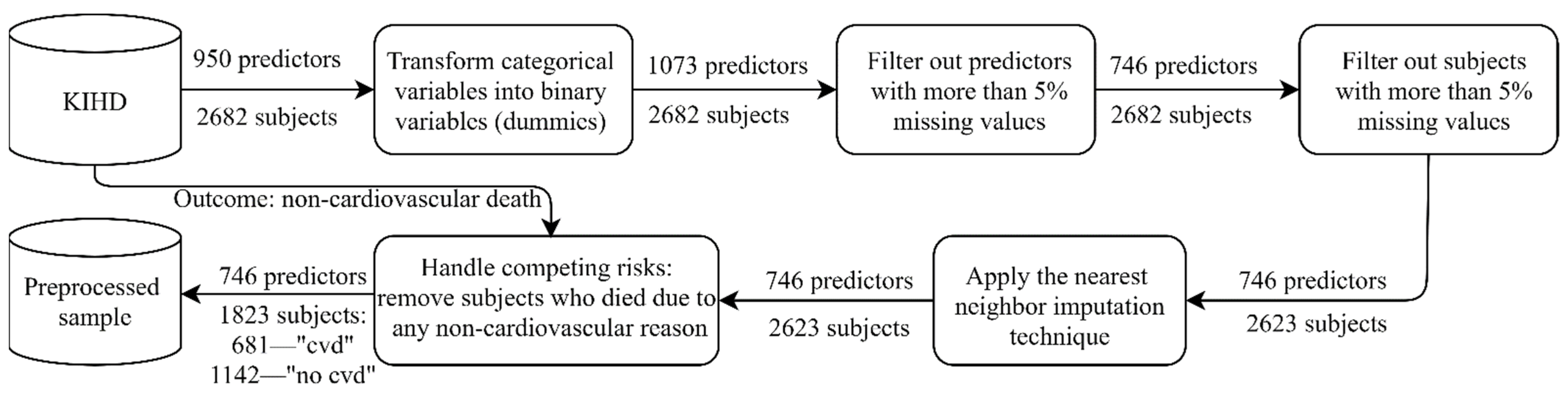
2.1. KIHD: Baseline Cohort
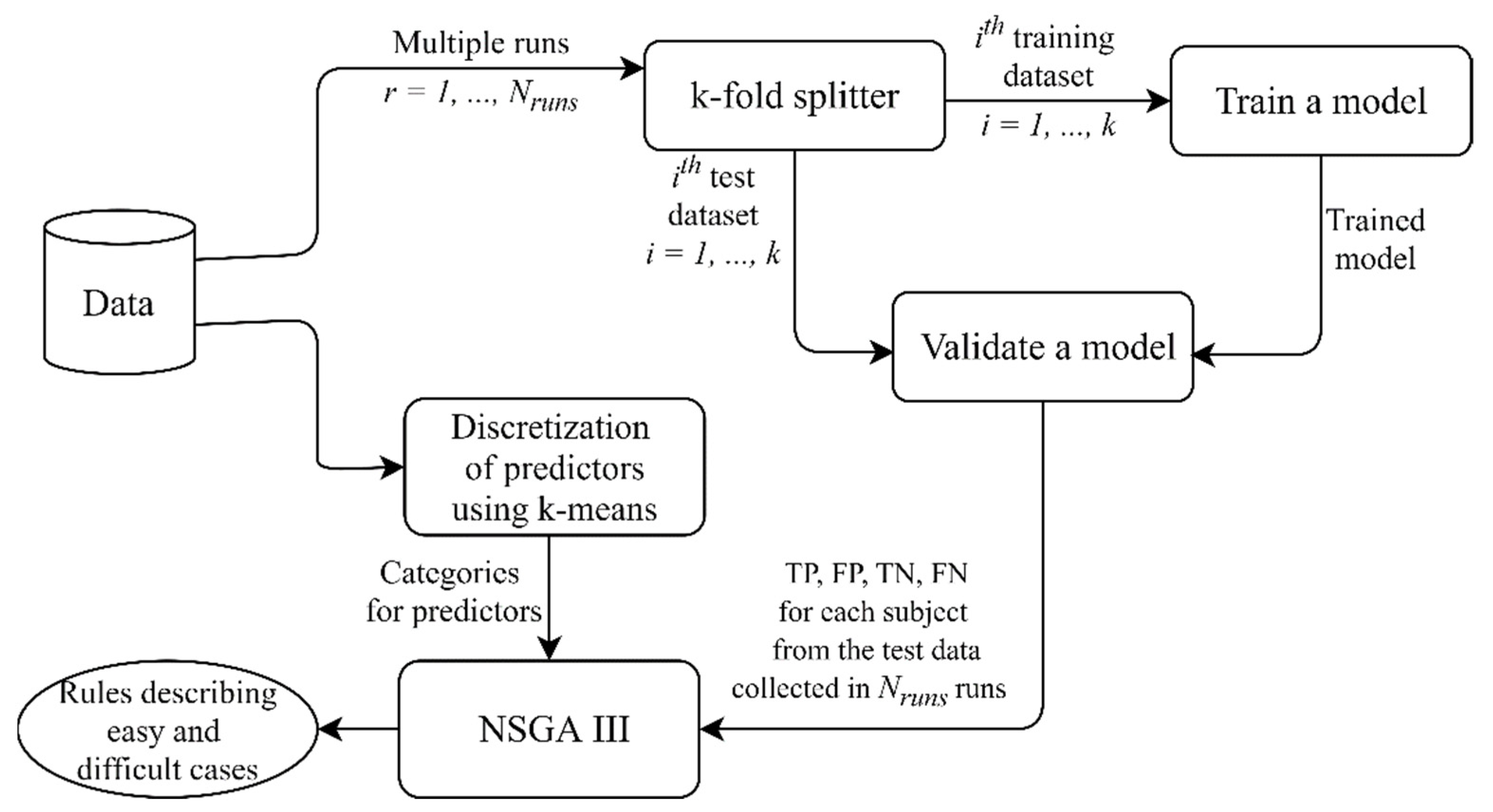
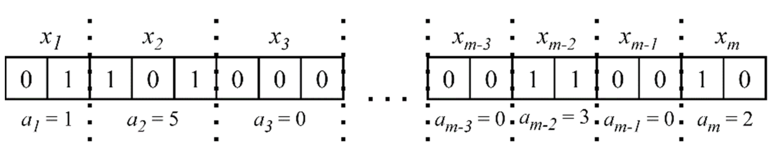
2.2. Multi-Objective Rule Design for the Model Post-Analysis
- There are at least subjects covered by the rule (the minimum rule support): = 30.
- The difference between TPR and TNR does not exceed ): (the rule is equally valid for “positive” and “negative” cases).
- The average model accuracy for subjects covered by the rule is either lower than or higher than (to define “difficult” and “easy” cases correspondingly): , .
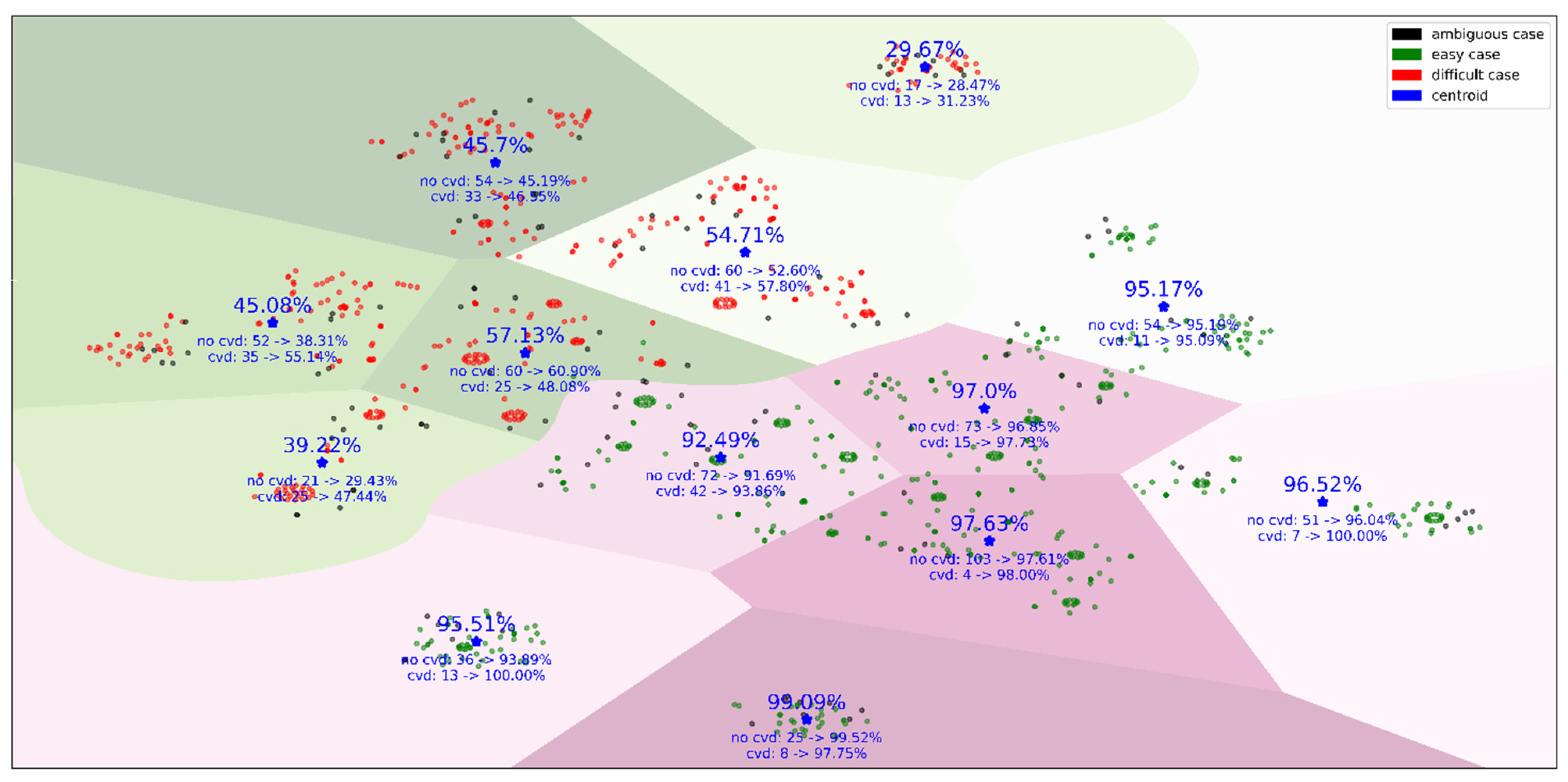
3. Results
4. Discussion
Supplementary Materials
Author Contributions
Funding
Institutional Review Board Statement
Informed Consent Statement
Data Availability Statement
Conflicts of Interest
References
- Kagiyama, N.; Shrestha, S.; Farjo, P.D.; Sengupta, P.P. Artificial intelligence: Practical primer for clinical research in cardiovascular disease. J. Am. Heart Assoc. 2019, 8, e012788. [Google Scholar] [CrossRef] [PubMed]
- Gulshan, V.; Peng, L.; Coram, M.; Stumpe, M.C.; Wu, D.; Narayanaswamy, A.; Venugopalan, S.; Widner, K.; Madams, T.; Cuadros, J.; et al. Development and validation of a deep learning algorithm for detection of diabetic retinopathy in retinal fundus photographs. JAMA 2016, 316, 2402–2410. [Google Scholar] [CrossRef] [PubMed]
- Verghese, A.; Shah, N.H.; Harrington, R.A. What this computer needs is a physician: Humanism and artificial intelligence. JAMA 2018, 319, 19–20. [Google Scholar] [CrossRef] [PubMed]
- Stead, W.W. Clinical implications and challenges of artificial intelligence and deep learning. JAMA 2018, 320, 1107–1108. [Google Scholar] [CrossRef] [PubMed]
- Stiglic, G.; Kocbek, P.; Fijacko, N.; Zitnik, M.; Verbert, K.; Cilar, L. Interpretability of machine learning-based prediction models in healthcare. WIREs Data Min. Knowl. Discov. 2020, e1379. [Google Scholar] [CrossRef]
- Interpretable Machine Learning. A Guide for Making Black Box Models Explainable. Available online: https://christophm.github.io/interpretable-ml-book/ (accessed on 14 December 2020).
- Ribeiro, M.T.; Singh, S.; Guestrin, C. Model-agnostic interpretability of machine learning. In Proceedings of the 2016 ICML Workshop on Human Interpretability in Machine Learning (WHI 2016), New York, NY, USA, 23 June 2016. [Google Scholar]
- Cava, W.; Bauer, C.; Moore, J.H.; Pendergrass, S.A. Interpretation of machine learning predictions for patient outcomes in electronic health records. AMIA Annu. Symp. Proc. 2020, 2019, 572–581. [Google Scholar]
- Koh, P.W.; Liang, P. Understanding black-box predictions via influence functions. In Proceedings of the 34th International Conference on Machine Learning, Sydney, Australia, 6–11 August 2017. [Google Scholar]
- Aguilera-Rueda, V.J.; Cruz-Ramírez, N.; Mezura-Montes, E. Data-driven Bayesian Network learning: A bi-objective approach to address the bias-variance decomposition. Math. Comput. Appl. 2020, 25, 37. [Google Scholar] [CrossRef]
- Ghose, A.; Ravindran, B. Interpretability with accurate small models. Front. Artif. Intell. 2020, 3, 3. [Google Scholar] [CrossRef] [Green Version]
- Veiga, R.V.; Barbosa, H.J.C.; Bernardino, H.S.; Freitas, J.M.; Feitosa, C.A.; Matos, S.M.A.; Alcântara-Neves, N.M.; Barreto, M.L. Multiobjective grammar-based genetic programming applied to the study of asthma and allergy epidemiology. BMC Bioinform. 2018, 19, 245. [Google Scholar] [CrossRef]
- Responsible-AI-Widgets. Available online: https://github.com/microsoft/responsible-ai-widgets/ (accessed on 11 June 2021).
- Singla, S.; Nushi, B.; Shah, S.; Kamar, E.; Horvitz, E. Understanding Failures of Deep Networks via Robust Feature Extraction. arXiv 2021, arXiv:2012.01750v2. Available online: https://arxiv.org/abs/2012.01750v2 (accessed on 22 June 2021).
- Sajeev, S.; Champion, S.; Beleigoli, A.; Chew, D.; Reed, R.L.; Magliano, D.J.; Shaw, J.E.; Milne, R.L.; Appleton, S.; Gill, T.K.; et al. Predicting Australian adults at high risk of cardiovascular disease mortality using standard risk factors and machine learning. Int. J. Environ. Res. Public Health 2021, 18, 3187. [Google Scholar] [CrossRef] [PubMed]
- Myers, P.D.; Ng, K.; Severson, K.; Kartoun, U.; Dai, W.; Huang, W.; Anderson, F.A.; Stultz, C.M. Identifying unreliable predictions in clinical risk models. NPJ Digit. Med. 2020, 3, 8. [Google Scholar] [CrossRef] [PubMed] [Green Version]
- Salonen, J.T. Is there a continuing need for longitudinal epidemiologic research? The Kuopio Ischaemic Heart Disease Risk Factor Study. Ann. Clin. Res. 1988, 20, 46–50. [Google Scholar] [PubMed]
- Kauhanen, J. Kuopio Ischemic Heart Disease Risk Factor Study. In Encyclopedia of Behavioral Medicine; Gellman, M.D., Turner, J.R., Eds.; Springer: New York, NY, USA, 2013. [Google Scholar] [CrossRef]
- International Statistical Classification of Diseases and Related Health Problems. 10th Revision (ICD-10). Available online: https://icd.who.int/browse10/2016/en#/IX (accessed on 25 October 2020).
- Troyanskaya, O.; Cantor, M.; Sherlock, G.; Brown, P.; Hastie, T.; Tibshirani, R.; Botstein, D.; Altman, R.B. Missing value estimation methods for DNA microarrays. Bioinformatics 2001, 17, 520–525. [Google Scholar] [CrossRef] [Green Version]
- Brester, C.; Voutilainen, A.; Tuomainen, T.P.; Kauhanen, J.; Kolehmainen, M. Epidemiological predictive modeling: Lessons learned from the Kuopio Ischemic Heart Disease Risk Factor Study. Inform. Health Soc. Care. under review.
- Hosmer, D.W.; Lemeshow, S. Applied Logistic Regression, 2nd ed.; John Wiley & Sons, Inc.: New York, NY, USA, 2000. [Google Scholar]
- Tibshirani, R. Regression shrinkage and selection via the lasso. J. R. Stat. Soc. Ser. B 1996, 58, 267–288. [Google Scholar] [CrossRef]
- Pedregosa, F.; Varoquaux, G.; Gramfort, A.; Michel, V.; Thirion, B.; Grisel, O.; Blondel, M.; Prettenhofer, P.; Weiss, R.; Dubourg, V.; et al. Scikit-learn: Machine learning in Python. JMLR 2011, 12, 2825–2830. [Google Scholar]
- Deb, K.; Jain, H. An evolutionary many-objective optimization algorithm using reference-point-based nondominated sorting approach, part I: Solving problems with box constraints. IEEE Trans. Evol. Comput. 2014, 18, 577–601. [Google Scholar] [CrossRef]
- Platypus. A Free and Open Source PYTHON library for Multiobjective Optimization. Available online: https://github.com/Project-Platypus/Platypus (accessed on 25 October 2020).
- Intelligent System for Model Design (isMODE) in Personalized Medicine. Available online: https://github.com/christinabrester/isMode (accessed on 14 December 2020).
- Curry, D.M.; Dagli, C.H. Computational complexity measures for many-objective optimization problems. Procedia Comput. Sci. 2014, 36, 185–191. [Google Scholar] [CrossRef] [Green Version]
- van der Maaten, L.J.P.; Hinton, G.E. Visualizing data using t-SNE. JMLR 2008, 9, 2579–2605. [Google Scholar]
- Chang, C.C.; Lin, C.J. LIBSVM: A library for support vector machines. ACM Trans. Intell. Syst. Technol. 2011, 2, 1–27. [Google Scholar] [CrossRef]
- Hastie, T.; Tibshirani, R.; Friedman, J.H. The Elements of Statistical Learning: Data Mining, Inference, and Prediction, 2nd ed.; Springer: New York, NY, USA, 2009. [Google Scholar]
- Pajouheshnia, R.; Damen, J.; Groenwold, R.; Moons, K.; Peelen, L. Treatment use in prognostic model research: A systematic review of cardiovascular prognostic studies. Diagn. Progn. Res. 2017, 1, 15. [Google Scholar] [CrossRef] [PubMed] [Green Version]
- Yang, L.; Wu, H.; Jin, X.; Zheng, P.; Hu, S.; Xu, X.; Yu, W.; Yan, J. Study of cardiovascular disease prediction model based on random forest in eastern China. Sci. Rep. 2020, 10, 5245. [Google Scholar] [CrossRef] [PubMed] [Green Version]
- Huang, Y.-C.; Li, S.-J.; Chen, M.; Lee, T.-S.; Chien, Y.-N. Machine-Learning Techniques for Feature Selection and Prediction of Mortality in Elderly CABG Patients. Healthcare 2021, 9, 547. [Google Scholar] [CrossRef] [PubMed]
- Alaa, A.M.; Bolton, T.; Di Angelantonio, E.; Rudd, J.; van der Schaar, M. Cardiovascular disease risk prediction using automated machine learning: A prospective study of 423,604 UK Biobank participants. PLoS ONE 2019, 14, e0213653. [Google Scholar] [CrossRef] [PubMed] [Green Version]
- Rezaee, M.; Putrenko, I.; Takeh, A.; Ganna, A.; Ingelsson, E. Development and validation of risk prediction models for multiple cardiovascular diseases and Type 2 diabetes. PLoS ONE 2020, 15, e0235758. [Google Scholar] [CrossRef]
- Responsible Machine Learning with Error Analysis. Available online: https://towardsdatascience.com/responsible-machine-learning-with-error-analysis-a7553f649915 (accessed on 11 June 2021).


| Setting (Parameter) Names | Setting (Parameter) Values |
|---|---|
| Selection | Tournament selection with a tournament size of 2 |
| Crossover | Half-uniform crossover |
| Mutation | Bin-flip mutation |
| Solution representation | Binary code Gray code |
| -objective problem | 3 |
| Outer divisions, | 20 |
| Inner divisions, | 0 |
| Reference points, | |
| Population size | The smallest multiple of four greater than , i.e., 232 |
| Generations | 200 |
| Probability distribution for initializing solutions in the starting population |
| Accuracy, % | The Number of Cases | ||||||
|---|---|---|---|---|---|---|---|
| Easy | Difficult | Ambiguous and Non-Covered | Easy | Difficult | Ambiguous | Non-Covered | |
| No cvd | 95.73 | 46.76 | 66.55 | 414 | 264 | 91 | 373 |
| Cvd | 96.28 | 50.17 | 76.05 | 100 | 172 | 31 | 378 |
| Overall | 95.84 | 48.11 | 71.00 | 514 (28.20%) | 436 (23.92%) | 122 (6.69%) | 751 (41.20%) |
Publisher’s Note: MDPI stays neutral with regard to jurisdictional claims in published maps and institutional affiliations. |
© 2021 by the authors. Licensee MDPI, Basel, Switzerland. This article is an open access article distributed under the terms and conditions of the Creative Commons Attribution (CC BY) license (https://creativecommons.org/licenses/by/4.0/).
Share and Cite
Brester, C.; Voutilainen, A.; Tuomainen, T.-P.; Kauhanen, J.; Kolehmainen, M. Post-Analysis of Predictive Modeling with an Epidemiological Example. Healthcare 2021, 9, 792. https://doi.org/10.3390/healthcare9070792
Brester C, Voutilainen A, Tuomainen T-P, Kauhanen J, Kolehmainen M. Post-Analysis of Predictive Modeling with an Epidemiological Example. Healthcare. 2021; 9(7):792. https://doi.org/10.3390/healthcare9070792
Chicago/Turabian StyleBrester, Christina, Ari Voutilainen, Tomi-Pekka Tuomainen, Jussi Kauhanen, and Mikko Kolehmainen. 2021. "Post-Analysis of Predictive Modeling with an Epidemiological Example" Healthcare 9, no. 7: 792. https://doi.org/10.3390/healthcare9070792
APA StyleBrester, C., Voutilainen, A., Tuomainen, T.-P., Kauhanen, J., & Kolehmainen, M. (2021). Post-Analysis of Predictive Modeling with an Epidemiological Example. Healthcare, 9(7), 792. https://doi.org/10.3390/healthcare9070792