
Evaluating Machine Learning Stability in Predicting Depression and Anxiety Amidst Subjective Response Errors


Abstract
1. Introduction
2. Related Review
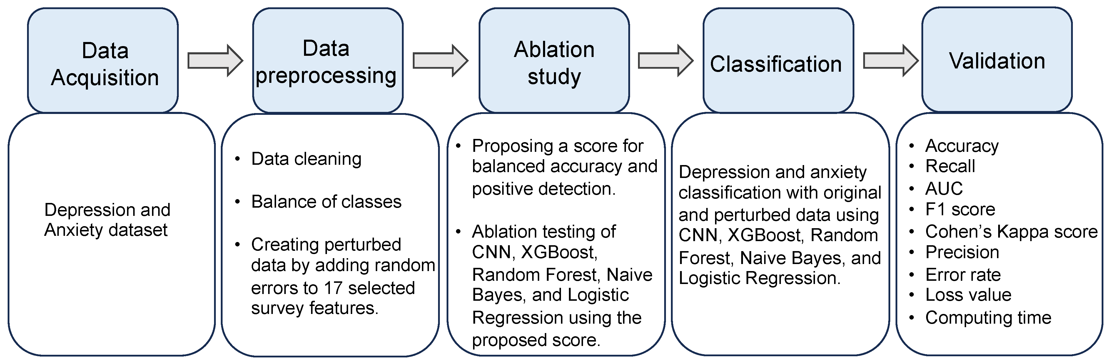
3. Methods
3.1. Participants
3.2. Measures
3.3. Psychiatric Diagnoses
3.4. Data with Unreliability
3.5. Data Preprocessing
3.6. Algorithms’ Description
- Forward Pass (CNN): Computation of predictions using current parameters .
- Loss Calculation (CNN): Computation of the loss based on and true labels .
- Backward Pass (CNN): Calculation of gradients .
- Parameter Update (CNN): Adjustment of using gradients .
- Callback Adjustment (CNN): Update the best model parameter for the next epoch based on the gradients and the composite score at time and adjust hyperparameters such as learning rate if a callback condition is met, based on composite score .
- Prediction (CNN): Make predictions after training.
- Update biased first moment estimate:
- Update biased second raw moment estimate:
- Compute bias-corrected first moment estimate:
- Compute bias-corrected second raw moment estimate:
- Update the parameters:
- Input Processing: The input data are preprocessed to match the input size expected by the network and are often normalized or standardized based on the same criteria used during training.
- Forward Propagation: The preprocessed input is then fed forward through the network’s layers, including convolutional layers, activation functions, pooling layers, and fully connected layers. Since dropout is not used during prediction, all neurons participate in computing the forward pass.
- Activation Function: The final layer’s activation function is interpreted as the prediction.
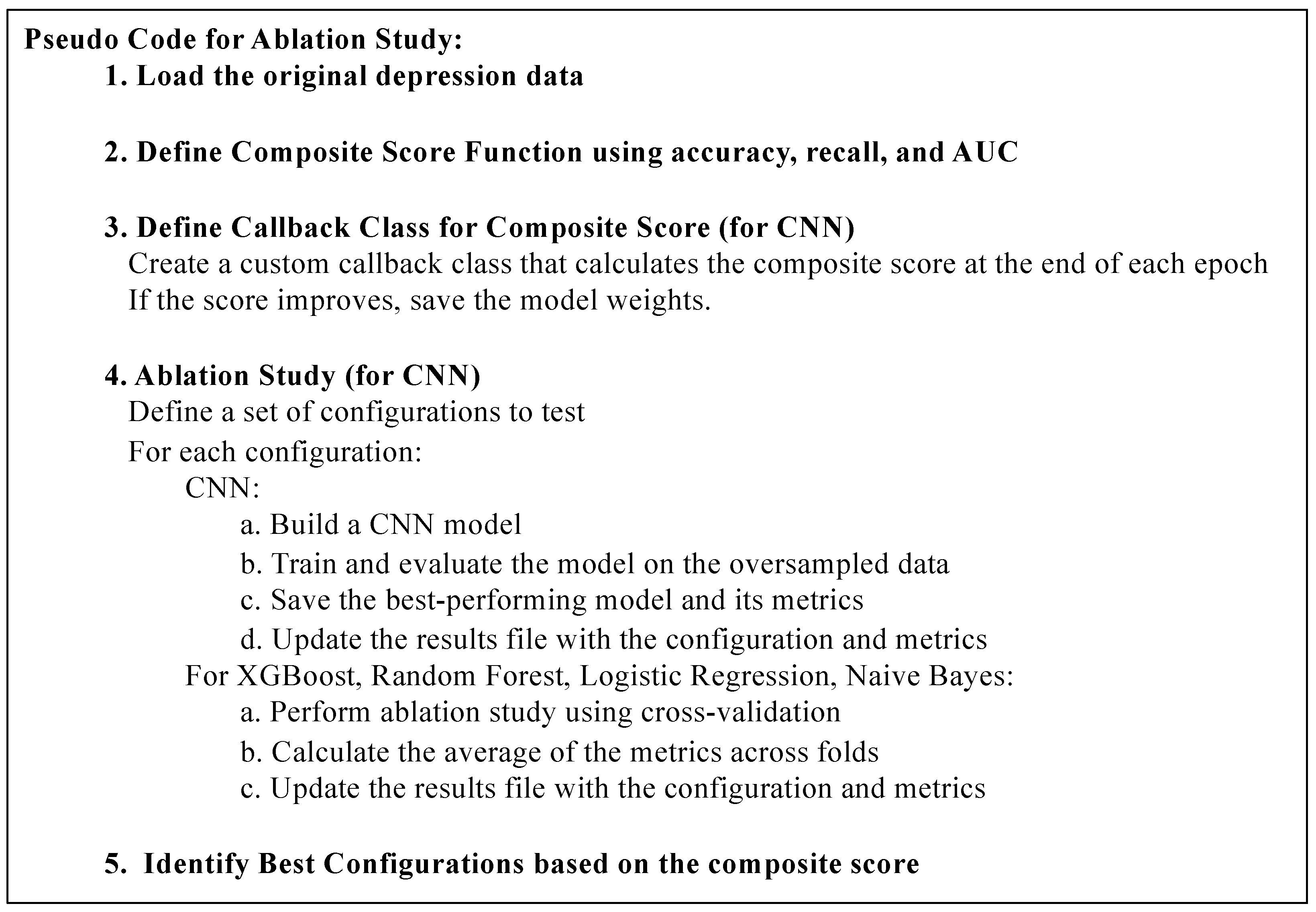
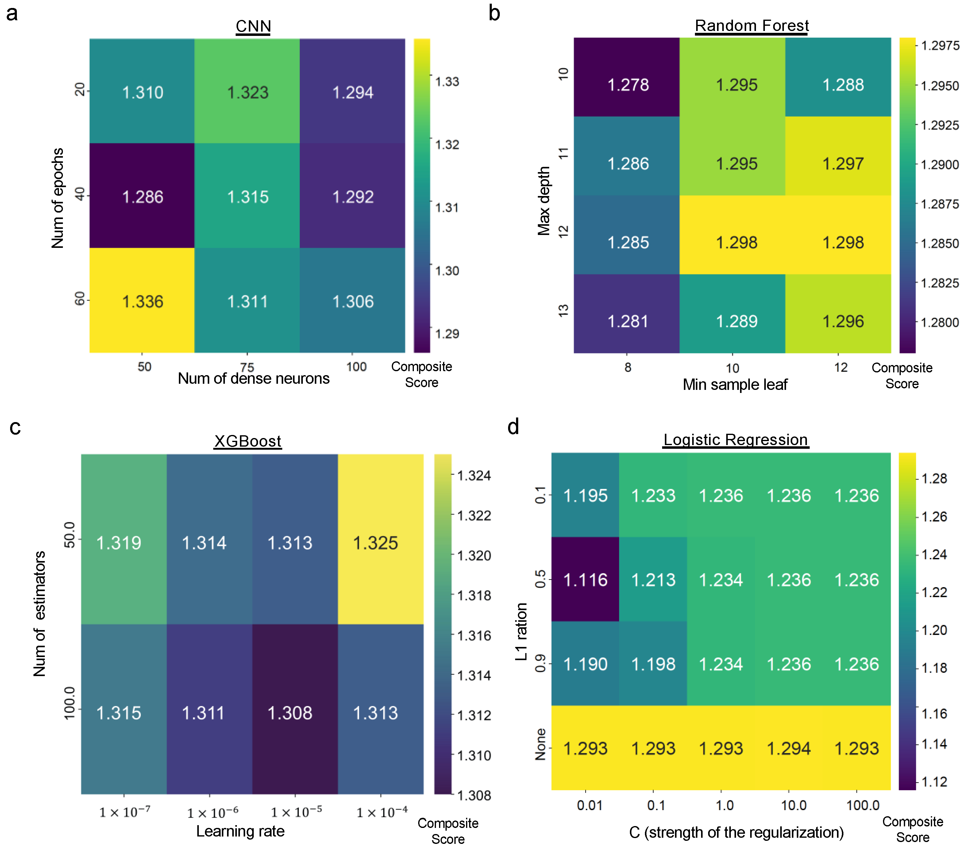
3.7. Ablation Study
3.8. Methods for Imbalanced Data
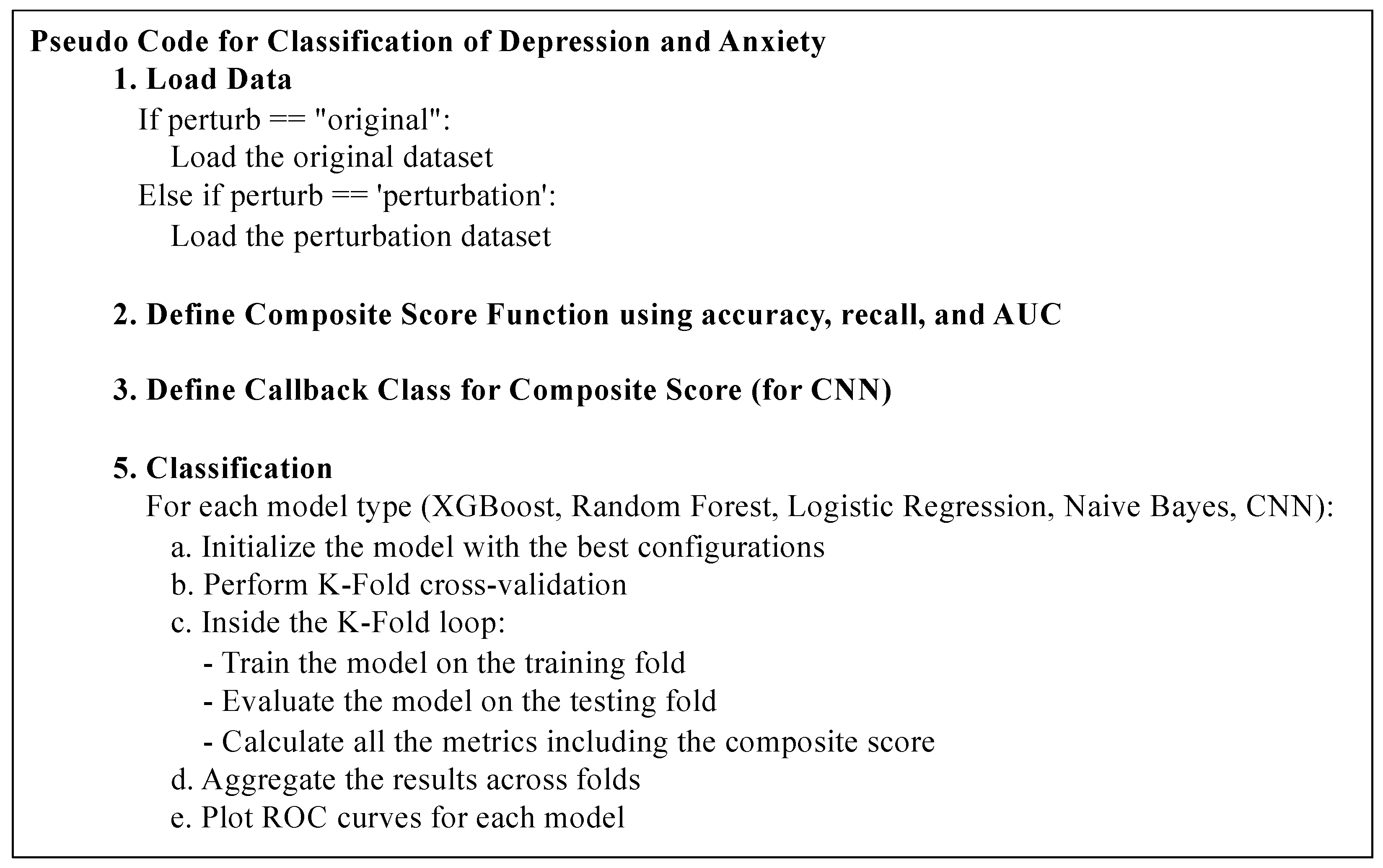
3.9. Model Training and Validation
3.10. Model Evaluation
3.11. System Configuration for Model Training
4. Results
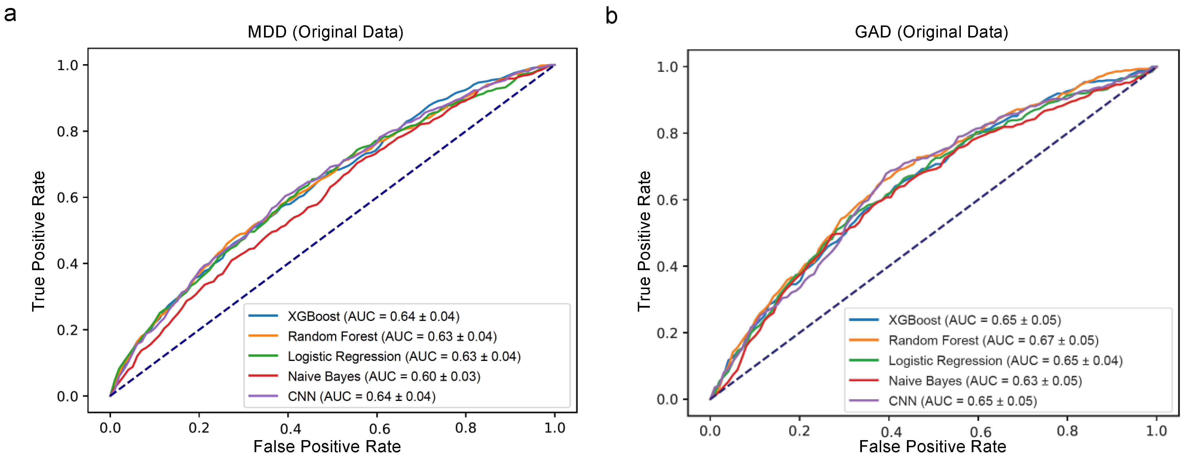
4.1. Predictive Performance for the Original Dataset
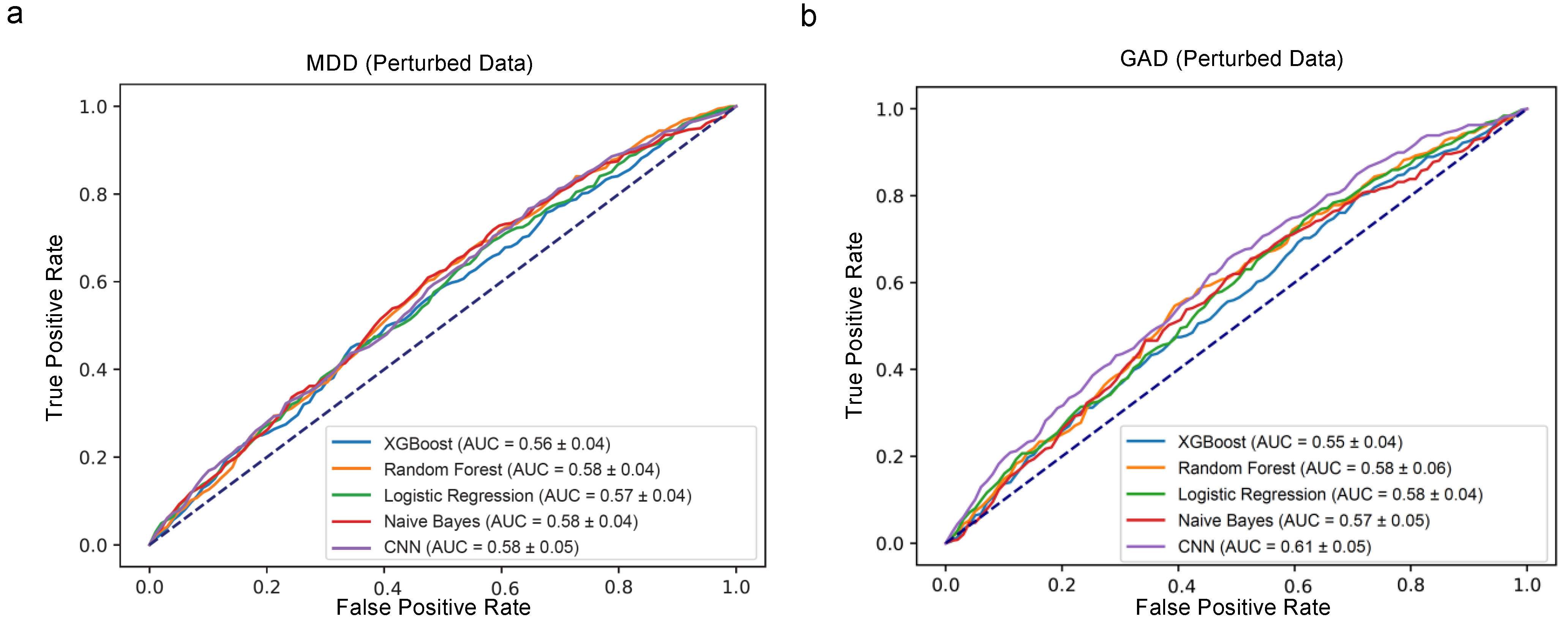
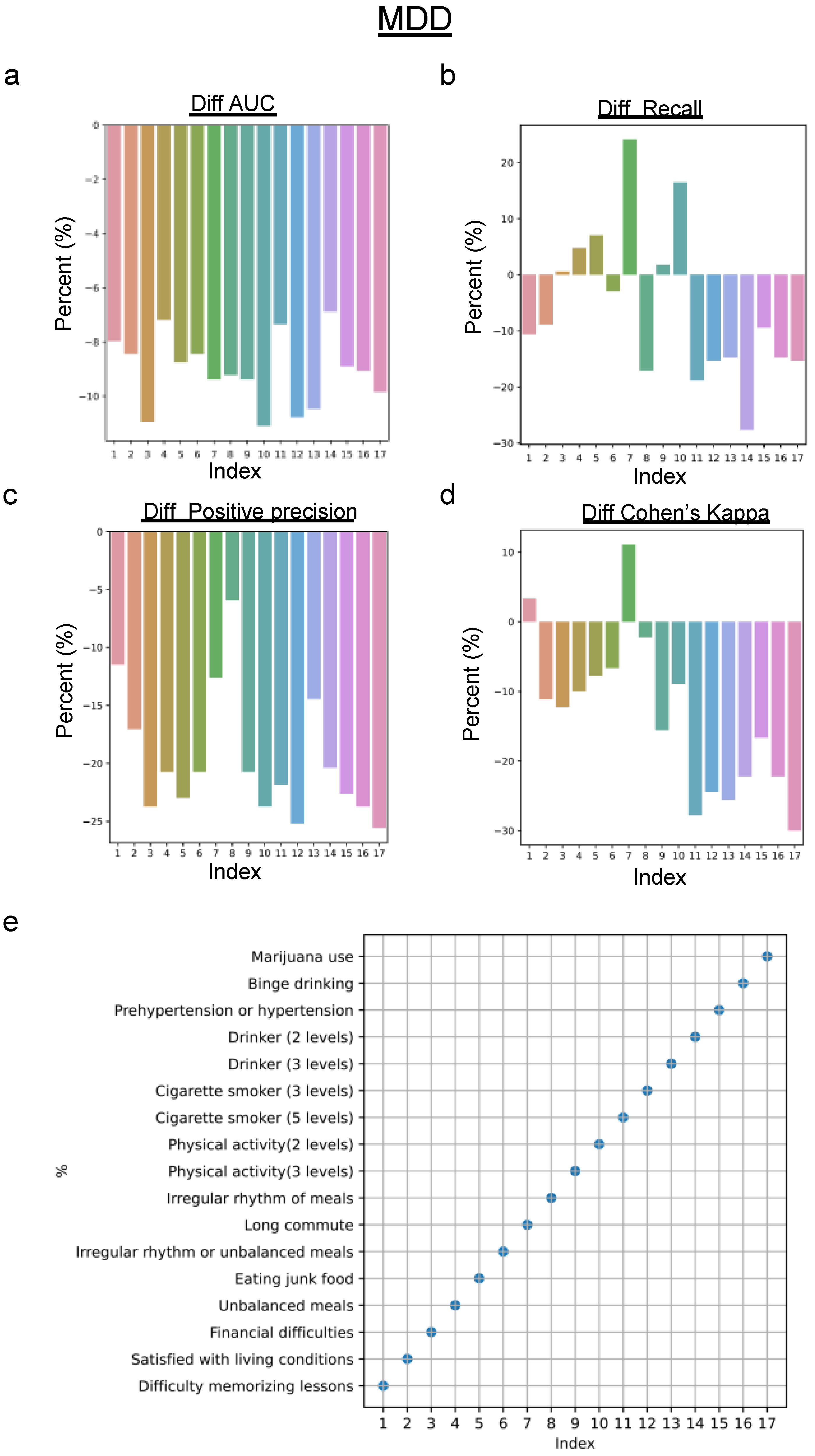
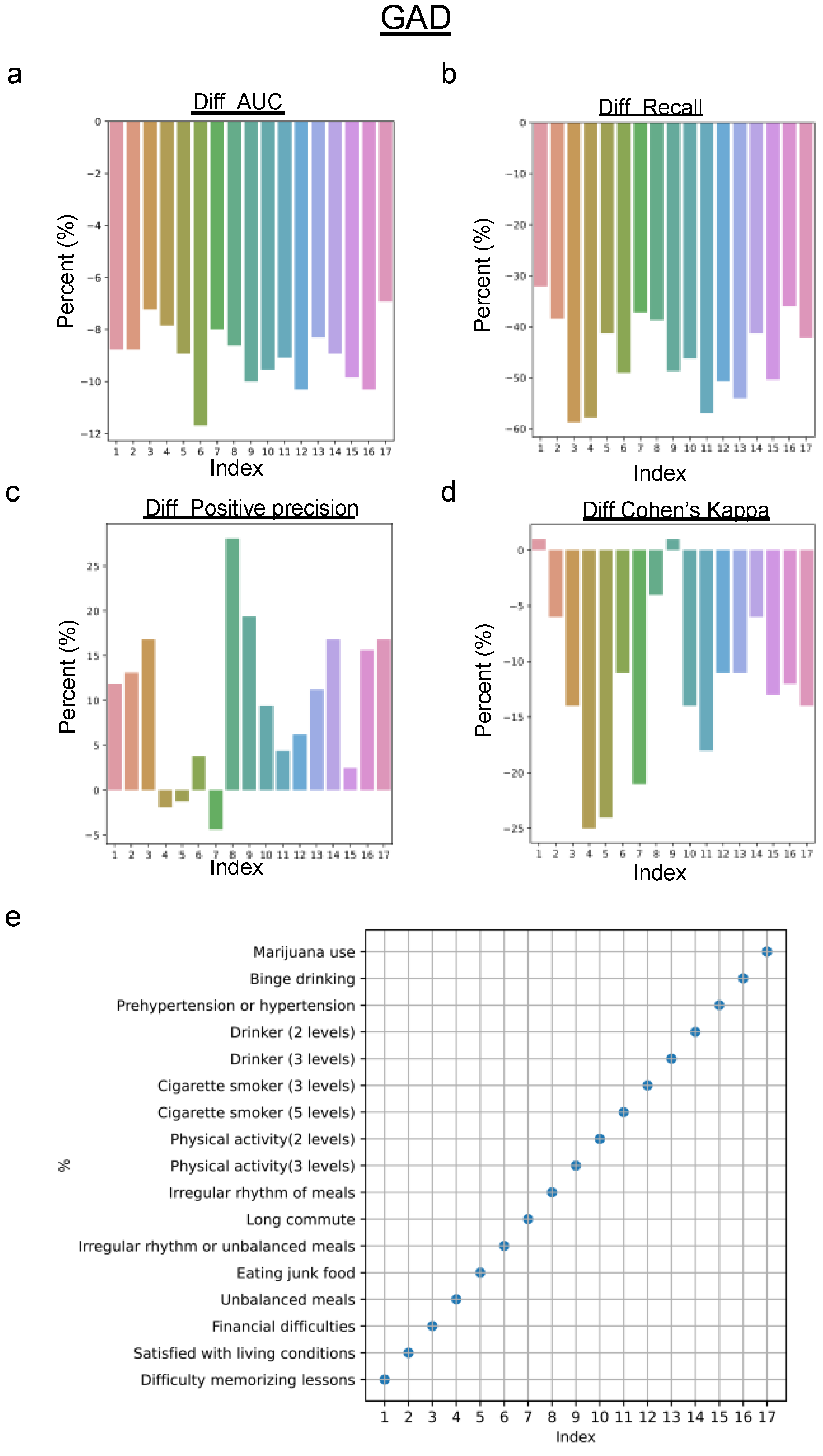
4.2. Predictive Performance for the Biased Dataset
5. Discussion
6. Conclusions
- Disease Prevention: Utilizing ML to analyze patterns in lifestyle and genetic data could lead to early identification of risk factors for chronic diseases, such as diabetes and heart disease, enabling preventative measures to be implemented sooner.
- Symptom Prediction: ML can be applied to predict the onset of symptoms for diseases like Alzheimer’s and Parkinson’s based on subtle changes in behavior or biomarkers, facilitating early intervention.
- Personalized Treatment Plans: By analyzing patient data, ML algorithms can help tailor treatment plans to individual needs, improving outcomes in conditions ranging from cancer to depression.
- Infection Outbreak Prediction: ML can be instrumental in predicting the outbreak of infectious diseases by analyzing travel, climate, and health data, allowing for timely public health responses.
Author Contributions
Funding
Institutional Review Board Statement
Informed Consent Statement
Data Availability Statement
Conflicts of Interest
References
- Zhou, Y.; Cao, Z.; Yang, M.; Xi, X.; Guo, Y.; Fang, M.; Cheng, L.; Du, Y. Comorbid generalized anxiety disorder and its association with quality of life in patients with major depressive disorder. Sci. Rep. 2017, 7, 40511. [Google Scholar] [CrossRef]
- Margoni, M.; Preziosa, P.; Rocca, M.A.; Filippi, M. Depressive symptoms, anxiety and cognitive impairment: Emerging evidence in multiple sclerosis. Transl. Psychiatry 2023, 13, 264. [Google Scholar] [CrossRef]
- Kraus, C.; Kadriu, B.; Lanzenberger, R.; Zarate, C.A.; Kasper, S. Prognosis and Improved Outcomes in Major Depression: A Review. Focus 2020, 18, 220–235. [Google Scholar] [CrossRef]
- Schroeders, U.; Schmidt, C.; Gnambs, T. Detecting Careless Responding in Survey Data Using Stochastic Gradient Boosting. Educ. Psychol. Meas. 2022, 82, 29–56. [Google Scholar] [CrossRef] [PubMed]
- Gianfrancesco, M.A.; Tamang, S.; Yazdany, J.; Schmajuk, G. Potential Biases in Machine Learning Algorithms Using Electronic Health Record Data. JAMA Intern. Med. 2018, 178, 1544–1547. [Google Scholar] [CrossRef] [PubMed]
- O’Shea, K.; Nash, R. An Introduction to Convolutional Neural Networks. arXiv 2015, arXiv:1511.08458. [Google Scholar] [CrossRef]
- Yamashita, R.; Nishio, M.; Do, R.K.G.; Togashi, K. Convolutional neural networks: An overview and application in radiology. Insights Imaging 2018, 9, 611–629. [Google Scholar] [CrossRef]
- Hong, W.; Zhou, X.; Jin, S.; Lu, Y.; Pan, J.; Lin, Q.; Yang, S.; Xu, T.; Basharat, Z.; Zippi, M.; et al. A Comparison of XGBoost, Random Forest, and Nomograph for the Prediction of Disease Severity in Patients With COVID-19 Pneumonia: Implications of Cytokine and Immune Cell Profile. Front. Cell Infect. Microbiol. 2022, 12, 819267. [Google Scholar] [CrossRef]
- Sun, D.; Xu, J.; Wen, H.; Wang, D. Assessment of landslide susceptibility mapping based on Bayesian hyperparameter optimization: A comparison between logistic regression and random forest. Eng. Geol. 2021, 281, 105972. [Google Scholar] [CrossRef]
- Ulinnuha, N.; Sa’dyah, H.; Rahardjo, M. A Study of Academic Performance Using Random Forest, Artificial Neural Network, Naïve Bayesian and Logistic Regression. Available online: https://api.semanticscholar.org/CorpusID:201104984 (accessed on 3 March 2024).
- Liu, L.; Qiao, C.; Zha, J.R.; Qin, H.; Wang, X.R.; Zhang, X.Y.; Wang, Y.O.; Yang, X.M.; Zhang, S.L.; Qin, J. Early prediction of clinical scores for left ventricular reverse remodeling using extreme gradient random forest, boosting, and logistic regression algorithm representations. Front. Cardiovasc. Med. 2022, 9, 864312. [Google Scholar] [CrossRef]
- Xin, Y.; Ren, X. Predicting depression among rural and urban disabled elderly in China using a random forest classifier. BMC Psychiatry 2022, 22, 118. [Google Scholar] [CrossRef] [PubMed]
- Antoniadi, A.M.; Galvin, M.; Heverin, M.; Hardiman, O.; Mooney, C. Prediction of caregiver burden in amyotrophic lateral sclerosis: A machine learning approach using random forests applied to a cohort study. BMJ Open 2020, 10, e033109. [Google Scholar] [CrossRef] [PubMed]
- Priya, A.; Garg, S.; Tigga, N.P. Predicting Anxiety, Depression and Stress in Modern Life using Machine Learning Algorithms. Procedia Comput. Sci. 2020, 167, 1258–1267. [Google Scholar] [CrossRef]
- Haque, U.M.; Kabir, E.; Khanam, R. Detection of child depression using machine learning methods. PLoS ONE 2021, 16, e0261131. [Google Scholar] [CrossRef]
- Zhou, Z.; Luo, D.; Yang, B.X.; Liu, Z. Machine Learning-Based Prediction Models for Depression Symptoms Among Chinese Healthcare Workers During the Early COVID-19 Outbreak in 2020: A Cross-Sectional Study. Front. Psychiatry 2022, 13, 876995. [Google Scholar] [CrossRef]
- Sharma, A.; Verbeke, W.J.M.I. Improving Diagnosis of Depression With XGBOOST Machine Learning Model and a Large Biomarkers Dutch Dataset. Front. Big Data 2020, 3, 15. [Google Scholar] [CrossRef]
- Ghosal, S.; Jain, A. Depression and Suicide Risk Detection on Social Media using fastText Embedding and XGBoost Classifier. Procedia Comput. Sci. 2023, 218, 1631–1639. [Google Scholar] [CrossRef]
- Gomes, S.R.B.S.; von Schantz, M.; Leocadio-Miguel, M. Predicting depressive symptoms in middle-aged and elderly adults using sleep data and clinical health markers: A machine learning approach. Sleep. Med. 2023, 102, 123–131. [Google Scholar] [CrossRef]
- du Toit, C.; Tran, T.Q.B.; Deo, N.; Aryal, S.; Lip, S.; Sykes, R.; Manandhar, I.; Sionakidis, A.; Stevenson, L.; Pattnaik, H.; et al. Survey and Evaluation of Hypertension Machine Learning Research. J. Am. Heart Assoc. 2023, 12, e027896. [Google Scholar] [CrossRef]
- Tran, A.; Tran, L.; Geghre, N.; Darmon, D.; Rampal, M.; Brandone, D.; Gozzo, J.M.; Haas, H.; Rebouillat-Savy, K.; Caci, H.; et al. Health assessment of French university students and risk factors associated with mental health disorders. PLoS ONE 2017, 12, e0188187. [Google Scholar] [CrossRef]
- Tate, A.E.; McCabe, R.C.; Larsson, H.; Lundström, S.; Lichtenstein, P.; Kuja-Halkola, R. Predicting mental health problems in adolescence using machine learning techniques. PLoS ONE 2020, 15, e0230389. [Google Scholar] [CrossRef]
- Ram Kumar, R.P.; Polepaka, S. Performance Comparison of Random Forest Classifier and Convolution Neural Network in Predicting Heart Diseases. In Proceedings of the Third International Conference on Computational Intelligence and Informatics, Hyderabad, India, 28–29 December 2018; Springer: Singapore, 2020; pp. 683–691. [Google Scholar]
- Chung, J.; Teo, J. Single classifier vs. ensemble machine learning approaches for mental health prediction. Brain Inform. 2023, 10, 1. [Google Scholar] [CrossRef]
- Baba, A.; Bunji, K. Prediction of Mental Health Problem Using Annual Student Health Survey: Machine Learning Approach. JMIR Ment. Health 2023, 10, e42420. [Google Scholar] [CrossRef] [PubMed]
- Latvala, A.; Kuja-Halkola, R.; Rück, C.; D’Onofrio, B.M.; Jernberg, T.; Almqvist, C.; Mataix-Cols, D.; Larsson, H.; Lichtenstein, P. Association of Resting Heart Rate and Blood Pressure in Late Adolescence With Subsequent Mental Disorders: A Longitudinal Population Study of More Than 1 Million Men in Sweden. JAMA Psychiatry 2016, 73, 1268–1275. [Google Scholar] [CrossRef] [PubMed]
- Graham, S.; Depp, C.; Lee, E.E.; Nebeker, C.; Tu, X.; Kim, H.C.; Jeste, D.V. Artificial Intelligence for Mental Health and Mental Illnesses: An Overview. Curr. Psychiatry Rep. 2019, 21, 116. [Google Scholar] [CrossRef] [PubMed]
- Jamalirad, H.; Jajroudi, M. Prediction of Mental Health Support of Employee Perceiving by Using Machine Learning Methods. Stud. Health Technol. Inform. 2023, 302, 903–904. [Google Scholar] [PubMed]
- Lokeshkumar, R.; Mishra, O.A.; Kalra, S. Social media data analysis to predict mental state of users using machine learning techniques. J. Educ. Health Promot. 2021, 10, 301. [Google Scholar] [CrossRef] [PubMed]
- Garriga, R.; Mas, J.; Abraha, S.; Nolan, J.; Harrison, O.; Tadros, G.; Matic, A. Machine learning model to predict mental health crises from electronic health records. Nat. Med. 2022, 28, 1240–1248. [Google Scholar] [CrossRef]
- Shi, Q.; Cai, N.; Jiao, W. Monitoring and Evaluating College Students’ Mental Health Based on Big Data Analysis. Am. J. Health Behav. 2022, 46, 164–176. [Google Scholar] [CrossRef]
- Rezapour, M.; Hansen, L. A machine learning analysis of COVID-19 mental health data. Sci. Rep. 2022, 12, 14965. [Google Scholar] [CrossRef]
- Jacobucci, R.; Grimm, K.J. Machine Learning and Psychological Research: The Unexplored Effect of Measurement. Perspect. Psychol. Sci. 2020, 15, 809–816. [Google Scholar] [CrossRef]
- Althubaiti, A. Information bias in health research: Definition, pitfalls, and adjustment methods. J. Multidiscip. Healthc. 2016, 9, 211–217. [Google Scholar] [CrossRef]
- Popoola, A.A.; Frediani, J.K.; Hartman, T.J.; Paynabar, K. Mitigating underreported error in food frequency questionnaire data using a supervised machine learning method and error adjustment algorithm. BMC Med. Inform. Decis. Mak. 2023, 23, 178. [Google Scholar] [CrossRef] [PubMed]
- Snowden, L.R. Bias in mental health assessment and intervention: Theory and evidence. Am. J. Public Health 2003, 93, 239–243. [Google Scholar] [CrossRef] [PubMed]
- Abràmoff, M.D.; Tarver, M.E.; Loyo-Berrios, N.; Trujillo, S.; Char, D.; Obermeyer, Z.; Eydelman, M.B.; Foundational Principles of Ophthalmic Imaging and Algorithmic Interpretation Working Group of the Collaborative Community for Ophthalmic Imaging Foundation, Washington, DC; Maisel, W.H. Considerations for addressing bias in artificial intelligence for health equity. npj Digit. Med. 2023, 6, 170. [Google Scholar] [CrossRef] [PubMed]
- Wang, R.; Chaudhari, P.; Davatzikos, C. Bias in machine learning models can be significantly mitigated by careful training: Evidence from neuroimaging studies. Proc. Natl. Acad. Sci. USA 2023, 120, e2211613120. [Google Scholar] [CrossRef]
- Taniguchi, H.; Sato, H.; Shirakawa, T. A machine learning model with human cognitive biases capable of learning from small and biased datasets. Sci. Rep. 2018, 8, 7397. [Google Scholar] [CrossRef]
- Nguyen, D.K.; Lan, C.H.; Chan, C.L. Deep Ensemble Learning Approaches in Healthcare to Enhance the Prediction and Diagnosing Performance: The Workflows, Deployments, and Surveys on the Statistical, Image-Based, and Sequential Datasets. Int. J. Environ. Res. Public Health 2021, 18, 811. [Google Scholar] [CrossRef]
- Radwan, A.; Zaafarani, L.; Abudawood, J.; AlZahrani, F.; Fourati, F. Addressing Bias Through Ensemble Learning and Regularized Fine-Tuning. arXiv 2024, arXiv:2402.00910. [Google Scholar]
- Moradi, M.; Samwald, M. Evaluating the robustness of neural language models to input perturbations. arXiv 2021, arXiv:2108.12237. [Google Scholar]
- Niu, X.; Mathur, P.; Dinu, G.; Al-Onaizan, Y. Evaluating Robustness to Input Perturbations for Neural Machine Translation. arXiv 2020, arXiv:2005.00580. [Google Scholar]
- Lambert, M.; Schuster, T.; Kessel, M.; Atkinson, C. Robustness Analysis of Machine Learning Models Using Domain-Specific Test Data Perturbation. In Progress in Artificial Intelligence, EPIA 2023, 5–8 September 2023, Faial Island, Portugal; Moniz, N., Vale, Z., Cascalho, J., Silva, C., Sebastião, R., Eds.; Springer: Cham, Switzerland, 2023; pp. 158–170. [Google Scholar] [CrossRef]
- Sanghvi, D.E.; Zainal, N.H.; Newman, M.G. Trait self-acceptance mediates parental childhood abuse predicting depression and anxiety symptoms in adulthood. J. Anxiety Disord. 2023, 94, 102673. [Google Scholar] [CrossRef]
- Visconti di Oleggio Castello, M.; Taylor, M.; Cavanagh, P.; Gobbini, M.I. Idiosyncratic, Retinotopic Bias in Face Identification Modulated by Familiarity. eNeuro 2018, 5, ENEURO.0054-18.2018. [Google Scholar] [CrossRef] [PubMed]
- Schwarz, H.; Revilla, M.; Weber, W. Memory effects in repeated survey questions: Reviving the empirical investigation of the independent measurements assumption. Surv. Res. Methods 2020, 14, 325–344. [Google Scholar]
- Borland, R.; Partos, T.R.; Cummings, K.M. Recall bias does impact on retrospective reports of quit attempts: Response to Messer and Pierce. Nicotine Tob. Res. 2013, 15, 754–755. [Google Scholar] [CrossRef] [PubMed][Green Version]
- Bispo Júnior, J.P. Social desirability bias in qualitative health research. Rev. Saude Publica 2022, 56, 101. [Google Scholar] [CrossRef]
- Chawla, N.V.; Bowyer, K.W.; Hall, L.O.; Kegelmeyer, W.P. SMOTE: Synthetic Minority Over-sampling Technique. arXiv 2011, arXiv:1106.1813. [Google Scholar] [CrossRef]
- Lundberg, S.; Lee, S.-I. A Unified Approach to Interpreting Model Predictions. arXiv 2017, arXiv:1705.07874. [Google Scholar]
- Gillespie, M.L.; Rao, U. Relationships between Depression and Executive Functioning in Adolescents: The Moderating Role of Unpredictable Home Environment. J. Child. Fam. Stud. 2022, 31, 2518–2534. [Google Scholar] [CrossRef]
- Hannigan, L.J.; McAdams, T.A.; Eley, T.C. Developmental change in the association between adolescent depressive symptoms and the home environment: Results from a longitudinal, genetically informative investigation. J. Child. Psychol. Psychiatry 2017, 58, 787–797. [Google Scholar] [CrossRef] [PubMed]
- Gavrilescu, M.; Vizireanu, N. Predicting Depression, Anxiety, and Stress Levels from Videos Using the Facial Action Coding System. Sensors 2019, 19, 3693. [Google Scholar] [CrossRef] [PubMed]
- Tran, A.; Tran, L.; Geghre, N.; Darmon, D.; Rampal, M.; Brandone, D.; Gozzo, J.-M.; Rebouillat-Savy, K.; Caci, H.; Avillach, P. Data from: Health assessment of French university students and risk factors associated with mental health disorders [Dataset]. Dryad 2018. [Google Scholar] [CrossRef]


| Feature | Description | Value |
|---|---|---|
| Sample Size | Total number of participants | 4.18 × 10³ |
| Study Period | Dates of data collection | September 2012–June 2013 |
| Recruitment Source | University medical service (UMS) | N/A |
| Faculty Representation | Diversity of academic disciplines | Sciences, humanities, medicine, law, sports science, engineering, business |
| Gender Distribution | Percentage of female and male participants | Female: 57.4%, Male: 42.6% |
| Age Groups | Distribution of participants by age | Less than 18: 5%, 18: 36%, 19: 28%, 20 or older: 31% |
| MDD Prevalence | Percentage of participants diagnosed with depression | 1.20 × 10⁻¹ |
| GAD Prevalence | Percentage of participants diagnosed with anxiety | 8.00 × 10⁻² |
| Index | Survey Features |
|---|---|
| 1 | Difficulty memorizing lessons |
| 2 | Satisfied with living conditions |
| 3 | Financial difficulties |
| 4 | Unbalanced meals |
| 5 | Eating junk food |
| 6 | Irregular rhythm or unbalanced meals |
| 7 | Long commute |
| 8 | Irregular rhythm of meals |
| 9 | Physical activity (3 levels) |
| 10 | Physical activity (2 levels) |
| 14 | Cigarette smoker (5 levels) |
| 12 | Cigarette smoker (3 levels) |
| 13 | Drinker (3 levels) |
| 14 | Drinker (2 levels) |
| 15 | Prehypertension or hypertension |
| 16 | Binge drinking |
| 17 | Marijuana use |
| MDD (Original Data) | |||||||||
|---|---|---|---|---|---|---|---|---|---|
| Model | Accuracy | Recall | F1 Weighted | Cohen’s Kappa | Positive Precision | Negative Precision | Error Rate | Loss | Computing Time (s) |
| XGBoost | 0.71 ± 0.03 | 0.43 ± 0.05 | 0.75 ± 0.02 | 0.12 ± 0.04 | 0.2 ± 0.03 | 0.9 ± 0.02 | 0.29 ± 0.03 | 0.69 ± 0.0 | 0.14 ± 0.02 |
| Random Forest | 0.86 ± 0.02 | 0.11 ± 0.04 | 0.82 ± 0.02 | 0.1 ± 0.05 | 0.3 ± 0.11 | 0.88 ± 0.01 | 0.14 ± 0.02 | 0.52 ± 0.01 | 2.99 ± 0.11 |
| Logistic Regression | 0.62 ± 0.02 | 0.55 ± 0.08 | 0.68 ± 0.02 | 0.1 ± 0.05 | 0.18 ± 0.04 | 0.91 ± 0.02 | 0.38 ± 0.02 | 0.65 ± 0.02 | 0.24 ± 0.03 |
| Naive Bayes | 0.53 ± 0.05 | 0.6 ± 0.1 | 0.6 ± 0.04 | 0.05 ± 0.02 | 0.15 ± 0.02 | 0.9 ± 0.02 | 0.47 ± 0.05 | 0.92 ± 0.08 | 0.04 ± 0.0 |
| CNN | 0.82 ± 0.07 | 0.17 ± 0.13 | 0.8 ± 0.04 | 0.09 ± 0.06 | 0.27 ± 0.1 | 0.88 ± 0.02 | 0.18 ± 0.07 | 0.44 ± 0.08 | 228.93 ± 4.67 |
| GAD (Original Data) | |||||||||
|---|---|---|---|---|---|---|---|---|---|
| Model | Accuracy | Recall | F1 Weighted | Cohen’s Kappa | Positive Precision | Negative Precision | Error Rate | Loss | Computing Time (s) |
| XGBoost | 0.75 ± 0.03 | 0.4 ± 0.07 | 0.8 ± 0.02 | 0.1 ± 0.05 | 0.13 ± 0.03 | 0.94 ± 0.01 | 0.25 ± 0.03 | 0.69 ± 0.0 | 0.14 ± 0.02 |
| Random Forest | 0.9 ± 0.02 | 0.08 ± 0.03 | 0.88 ± 0.02 | 0.06 ± 0.05 | 0.17 ± 0.07 | 0.93 ± 0.01 | 0.1 ± 0.02 | 0.42 ± 0.01 | 2.99 ± 0.1 |
| Logistic Regression | 0.64 ± 0.03 | 0.58 ± 0.09 | 0.73 ± 0.02 | 0.08 ± 0.03 | 0.12 ± 0.02 | 0.95 ± 0.01 | 0.36 ± 0.03 | 0.64 ± 0.02 | 0.18 ± 0.04 |
| Naive Bayes | 0.68 ± 0.04 | 0.5 ± 0.13 | 0.76 ± 0.03 | 0.08 ± 0.04 | 0.12 ± 0.03 | 0.94 ± 0.01 | 0.32 ± 0.04 | 0.74 ± 0.1 | 0.04 ± 0.0 |
| CNN | 0.8 ± 0.1 | 0.32 ± 0.19 | 0.83 ± 0.06 | 0.1 ± 0.03 | 0.16 ± 0.05 | 0.94 ± 0.01 | 0.2 ± 0.1 | 0.46 ± 0.12 | 236.47 ± 5.02 |
| MDD (Perturbed Data) | |||||||||
|---|---|---|---|---|---|---|---|---|---|
| Model | Accuracy | Recall | F1 Weighted | Cohen’s Kappa | Positive Precision | Negative Precision | Error Rate | Loss | Computing Time (s) |
| XGBoost | 0.81 ± 0.02 | 0.13 ± 0.03 | 0.8 ± 0.02 | 0.04 ± 0.04 | 0.17 ± 0.06 | 0.88 ± 0.01 | 0.19 ± 0.02 | 0.69 ± 0.0 | 0.14 ± 0.03 |
| Random Forest | 0.87 ± 0.02 | 0.0 ± 0.0 | 0.82 ± 0.02 | 0.0 ± 0.0 | 0.0 ± 0.0 | 0.87 ± 0.02 | 0.13 ± 0.02 | 0.49 ± 0.01 | 2.95 ± 0.02 |
| Logistic Regression | 0.6 ± 0.02 | 0.48 ± 0.08 | 0.66 ± 0.02 | 0.05 ± 0.03 | 0.15 ± 0.03 | 0.89 ± 0.01 | 0.4 ± 0.02 | 0.67 ± 0.02 | 0.28 ± 0.03 |
| Naive Bayes | 0.45 ± 0.05 | 0.7 ± 0.07 | 0.52 ± 0.06 | 0.04 ± 0.02 | 0.15 ± 0.02 | 0.91 ± 0.02 | 0.55 ± 0.05 | 0.82 ± 0.07 | 0.04 ± 0.0 |
| CNN | 0.84 ± 0.03 | 0.1 ± 0.08 | 0.81 ± 0.02 | 0.06 ± 0.16 | 0.28 ± 0.16 | 0.88 ± 0.02 | 0.16 ± 0.03 | 0.44 ± 0.04 | 252.11 ± 5.38 |
| GAD (Perturbed Data) | |||||||||
|---|---|---|---|---|---|---|---|---|---|
| Model | Accuracy | Recall | F1 Weighted | Cohen’s Kappa | Positive Precision | Negative Precision | Error Rate | Loss | Computing Time (s) |
| XGBoost | 0.75 ± 0.06 | 0.27 ± 0.09 | 0.8 ± 0.04 | 0.04 ± 0.04 | 0.1 ± 0.03 | 0.93 ± 0.01 | 0.25 ± 0.06 | 0.69 ± 0.0 | 0.2 ± 0.02 |
| Random Forest | 0.92 ± 0.01 | 0.0 ± 0.0 | 0.89 ± 0.02 | 0.0 ± 0.0 | 0.0 ± 0.0 | 0.92 ± 0.01 | 0.08 ± 0.01 | 0.39 ± 0.01 | 6.95 ± 0.29 |
| Logistic Regression | 0.63 ± 0.02 | 0.44 ± 0.07 | 0.72 ± 0.01 | 0.03 ± 0.02 | 0.09 ± 0.02 | 0.93 ± 0.01 | 0.37 ± 0.02 | 0.66 ± 0.02 | 1.08 ± 0.2 |
| Naive Bayes | 0.51 ± 0.05 | 0.62 ± 0.09 | 0.62 ± 0.05 | 0.03 ± 0.03 | 0.09 ± 0.02 | 0.94 ± 0.02 | 0.49 ± 0.05 | 0.79 ± 0.04 | 0.08 ± 0.0 |
| CNN | 0.9 ± 0.02 | 0.08 ± 0.06 | 0.88 ± 0.02 | 0.07 ± 0.07 | 0.3 ± 0.27 | 0.93 ± 0.01 | 0.1 ± 0.02 | 0.31 ± 0.05 | 810.6 ± 16.78 |
| Study | Goal | Methods | Input Data | Model Performance | Comparison |
|---|---|---|---|---|---|
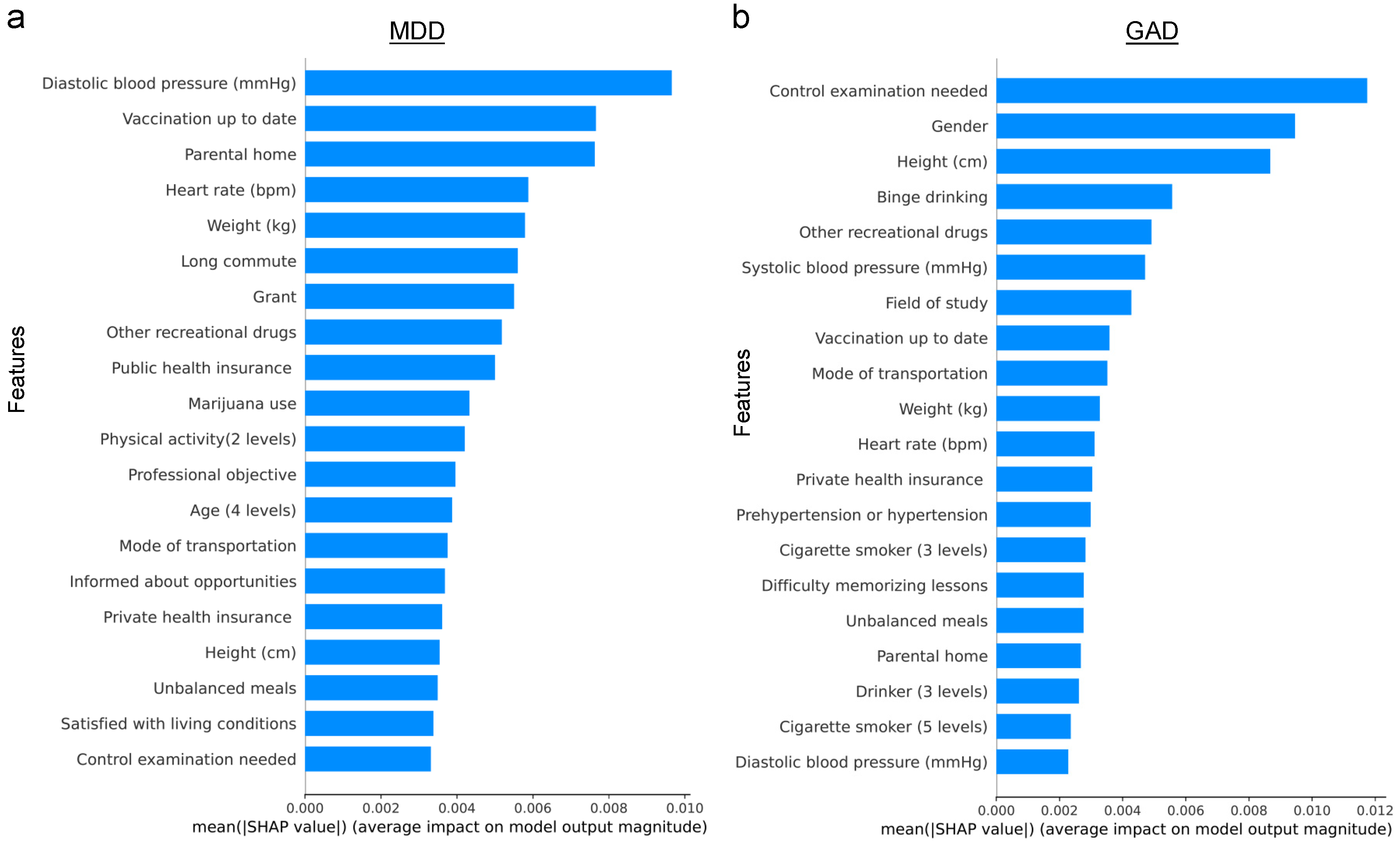
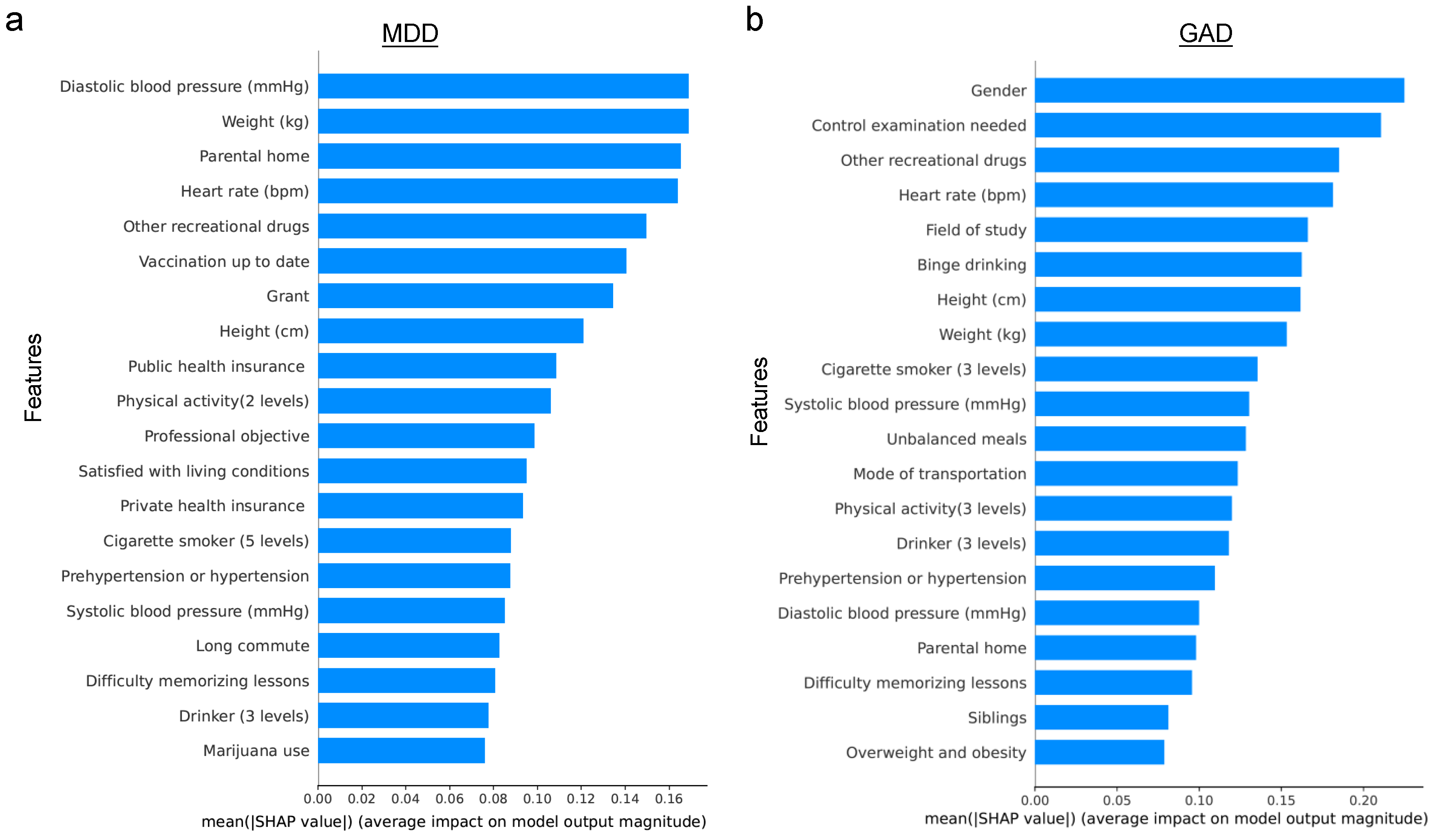
| The current study | Assess ML models’ reliability for mental health prediction with subjective data. | CNN, XGBoost, Random Forest, Logistic Regression, Naïve Bayes | Self-reported surveys from students (sociodemographics, health, lifestyle) | CNN best. High accuracy, resilience with biased data, specific features’ impact | NA |
| Single classifier vs. ensemble ML approaches for mental health prediction [24] | Evaluate ML algorithms for mental health prediction. | Logistic Regression, Gradient Boosting, Neural Networks, KNN, SVM, DNN, XGBoost, Ensemble approach | Open data set (OSMI Mental Health in Tech Survey) on mental health in tech industry | Gradient Boosting best, NN also good. Feature selection important (family history, age). | Similar use of ML in a different context (mental health in tech focusing on burnout and anxiety) resulted in different best models like Gradient Boosting for clean data and ensemble approaches for noisy data. |
| Prediction of Mental Health Problem Using Annual Student Health Survey: Machine Learning Approach [25] | Predict student mental health using health survey responses and response times. | Logistic Regression, Elastic Net, Random Forest, XGBoost, LightGBM | Responses to health surveys (demographics, survey answers, response time) | Elastic Net and LightGBM best, specific survey questions and response times impactful. | Similar use of ML in a different data (health surveys) resulted in different best models like Elastic Net and LightGBM |
| Predicting Mental Health Problems in Adolescence Using Machine Learning Techniques [22] | Develop a model for predicting mental health problems in adolescence using ML. | Random Forest, XGBoost, Logistic Regression, Neural Network, SVM | Parental report and register data (474 predictors), SDQ for mental health | Random forest and SVM best, but similar performance to Logistic Regression. Parental reports and environment important. | Their study and the current study both identified Random Forest as the best performing model, for data without added error. |
Disclaimer/Publisher’s Note: The statements, opinions and data contained in all publications are solely those of the individual author(s) and contributor(s) and not of MDPI and/or the editor(s). MDPI and/or the editor(s) disclaim responsibility for any injury to people or property resulting from any ideas, methods, instructions or products referred to in the content. |
© 2024 by the authors. Licensee MDPI, Basel, Switzerland. This article is an open access article distributed under the terms and conditions of the Creative Commons Attribution (CC BY) license (https://creativecommons.org/licenses/by/4.0/).
Share and Cite
Ku, W.L.; Min, H. Evaluating Machine Learning Stability in Predicting Depression and Anxiety Amidst Subjective Response Errors. Healthcare 2024, 12, 625. https://doi.org/10.3390/healthcare12060625
Ku WL, Min H. Evaluating Machine Learning Stability in Predicting Depression and Anxiety Amidst Subjective Response Errors. Healthcare. 2024; 12(6):625. https://doi.org/10.3390/healthcare12060625
Chicago/Turabian StyleKu, Wai Lim, and Hua Min. 2024. "Evaluating Machine Learning Stability in Predicting Depression and Anxiety Amidst Subjective Response Errors" Healthcare 12, no. 6: 625. https://doi.org/10.3390/healthcare12060625
APA StyleKu, W. L., & Min, H. (2024). Evaluating Machine Learning Stability in Predicting Depression and Anxiety Amidst Subjective Response Errors. Healthcare, 12(6), 625. https://doi.org/10.3390/healthcare12060625