Discrete Velocity Boltzmann Model for Quasi-Incompressible Hydrodynamics

Abstract

In this paper, we consider the development of the two-dimensional discrete velocity Boltzmann model on a nine-velocity lattice. Compared to the conventional lattice Boltzmann approach for the present model, the collision rules for the interacting particles are formulated explicitly. The collisions are tailored in such a way that mass, momentum and energy are conserved and the H-theorem is fulfilled. By applying the Chapman–Enskog expansion, we show that the model recovers quasi-incompressible hydrodynamic equations for small Mach number limit and we derive the closed expression for the viscosity, depending on the collision cross-sections. In addition, the numerical implementation of the model with the on-lattice streaming and local collision step is proposed. As test problems, the shear wave decay and Taylor–Green vortex are considered, and a comparison of the numerical simulations with the analytical solutions is presented.

1. Introduction

In the kinetic theory, the distribution function of a rarefied gaseous system is governed by the Boltzmann equation or its models [1]. In the applications, the discretization of these equations in the velocity (and physical) space is usually performed. One of the most popular discretization approaches is the Lattice–Boltzmann (LB) method [2,3,4,5] which was initially developed as an alternative to the continuum fluid methods like Navier–Stokes equations [6]; furthermore, the method has been extended to the rarefied flows modeling [7,8,9,10,11,12,13,14,15,16,17,18,19]. The conventional LB model has the following form

$$\frac{d{f}_i}{dt}=\frac{1}{\tau }(f_i^{eq}-f_i),i=1\dots N,$$

where $f_i(t,\mathit{x})$ is the distribution function related to the particles with the velocity ${\mathit{c}}_{\mathit{i}}$, $i=1\dots N$, $\tau$ is the relaxation time, $f_i^{eq}$ is the local equilibrium, N is the number of the discrete velocities, $\frac{d}{dt}=\frac{\partial }{\partial t}+$${\mathit{c}}_{\mathit{i}}\frac{\partial }{\partial \mathit{r}}$, $\mathit{r}$ is the spatial variable. In this approach, the collisions between the particles are described in a phenomenological way, i.e., it is postulated that, due to the collisions, the distribution function tends to the local equilibrium state at a rate proportional to $f_i^{eq}-f_i$. For LB models, the local equilibrium is usually taken as a finite-order polynomial on the bulk velocity, and the conservation laws for mass and momentum are satisfied by construction. On the other hand, for this form of the local equilibrium, the H-theorem does not exist [20,21,22]. To overcome this issue, models with non-polynomial equilibria have been proposed [23,24,25,26].

Another possible discretization technique is the discrete velocity (DV) Boltzmann method [27,28,29,30], the general DV Boltzmann model reads as

$$\frac{d{f}_i}{dt}=\sum _{jkl}^N{A}_{kl}^{ij}(f_k{f}_l-f_i{f}_j)\equiv I_i[f_1,\dots f_N],i=1\dots N,$$

(1)

where $A_{kl}^{ij}=A_{ij}^{kl}\ge 0$ are the transition probabilities.

Compared to the LB method, the DV models have some attractive properties. Similarly to the Boltzmann equation, the binary collisions are described explicitly. Moreover, by construction, the H-theorem is valid for these models [28], i.e.,

$$\frac{dH}{dt}\le 0,H\left(t\right)=\int d\mathit{r}\sum _i^N{f}_{i}log\left(f_i\right).$$

Moreover, the local equilibrium for DV kinetic Boltzmann models can be obtained as an exponential function of the macroscopic variables. The DV Boltzmann approach attracted the attention of many researchers several decades ago, but, at present, is significantly less popular than the LB method. For instance, the well-known four velocity Broadwell equation in two dimensions has been investigated thoroughly [31,32,33,34,35,36], this model has correct collision invariants, but its discrete velocity set is too small and lacks isotropy [37]; therefore, the correct description of the hydrodynamics is impossible in the framework of this model. In addition, another subtle feature should be mentioned: for the discrete velocity models, the molecular chaos hypothesis can be violated, i.e., the particles can be correlated before the collision [38]. This is undesirable, but the influence of this effect on the flow properties in applications is not clear. Furthermore, one should construct the DV Boltzmann models in such a way that the only conserved variables are mass, momentum and energy. The equilibrium state is obtained as minimum of the H-function under the constraint that these variables are not changed by collisions. The presence of other conserved quantities (spurious invariants) changes the form of the local equilibrium state, this, in turn, leads to a distortion of the hydrodynamic equations. The construction of DV Boltzmann models without excessive invariants is a non-trivial procedure [39,40,41,42].

In this paper we consider a DV Boltzmann model on a nine velocity, two-dimensional lattice. As a starting point, we consider the local equilibrium for the general DV Boltzmann model and its expansion at the vicinity of the absolute Maxwell distribution. Next, the Chapman–Enskog expansion for the DV Boltzmann model is performed in order to derive the hydrodynamic equations. In addition, we show that the model does not have invariants without physical meaning. The considered model has four different possible transition probabilities. In terms of the LB theory, this model can be considered as a scheme with multiple relaxation times. For viscosity, we obtain a closed expression depending on the values of the transition probabilities. If the viscosity is fixed, we obtain a constraint on the transition probabilities, but three of them can be chosen as free parameters; for instance, they can be adjusted to improve stability properties. As benchmark problems, we consider the shear wave decay and Taylor–Green vortex. The numerical experiments show excellent agreement between the numerical simulation results and analytical solutions.

2. Equilibrium for DV Boltzmann Kinetic Model and the Euler Equations

The local equilibrium of the model (1) is obtained as a minimum of the H functional with the constraints corresponding to the conservation laws; it has the following form (Formula (5) in [43])

$$f_i^{eq}=exp(a+\mathit{b}·{\mathit{c}}_{\mathit{i}}+d{c}_i^2),i=1\dots N,$$

(2)

where the coefficients $a_i,{\mathit{b}}_i,d_i$ depend on the density, flow velocityand temperature $\rho ,\mathit{u},\theta$ and “·” defines scalar product. In this paragraph, we consider the particle’s dynamics in D spatial dimensions. We assume that the local equilibrium is close to the absolute equilibrium with the density ${\rho }_0=1$ flow velocity $u_0=0$ and the temperature ${\theta }_0$; then, one can write down the absolute equilibrium denoted as $w_i$ in the form

$$w_i=exp(a^0+d^0{c}_i^2),i=1\dots N,$$

where $a^0=a^0({\rho }_0,{\theta }_0),d^0=d^0({\rho }_0,{\theta }_0)$, we also term $w_i$ as lattice weights. The conservation laws for mass, momentum, energy yield the following equations for the lattice velocities and the lattice weights

$$\sum _i{w}_i=1,\sum _i{w}_i{\mathit{c}}_{\mathit{i}}=0,\sum _i{w}_i{\mathit{c}}_{\mathit{i}}{\mathit{c}}_{\mathit{i}}={\theta }_0\mathit{\delta },$$

(3)

note that ${\mathit{c}}_{\mathit{i}}{\mathit{c}}_{\mathit{i}}$ is a tensor with elements $c_{i,\alpha }{c}_{i,\beta },\alpha ,\beta =1\dots D$, and that D is the number of spatial dimensions. For the coefficients, we have the expression

$$a_i=a_i^0+\Delta a,{\mathit{b}}_i=\Delta \mathit{b},d_i=d_i^0+\Delta d,$$

where $\Delta a,\Delta \mathit{b},\Delta d$ are small quantities. Similarly to the previous studies [43] we expand the expression (2) on $\Delta a,\Delta \mathit{b},\Delta d$, and one has

$$f_i^{eq}=w_i(1+\Delta a+\frac{1}{2}\Delta a^2+o(\Delta a^2))\times$$

$$\times (1+\Delta \mathit{b}·{\mathit{c}}_{\mathit{i}}+\frac{1}{2}\Delta \mathit{b}\Delta \mathit{b}:{\mathit{c}}_{\mathit{i}}{\mathit{c}}_{\mathit{i}}+o\left({\Delta \mathit{b}}^2\right))(1+\Delta d{c}_i^2+\frac{1}{2}\Delta d^2{c}_i^4+o(\Delta d^2))=$$

$$=w_i(1+\Delta a+\Delta \mathit{b}·{\mathit{c}}_{\mathit{i}}+\Delta d{c}_i^2+$$

$$+\frac{1}{2}\Delta a^2+\Delta a\Delta \mathit{b}·{\mathit{c}}_{\mathit{i}}+\Delta a\Delta d{c}_i^2+\frac{1}{2}\Delta \mathit{b}\Delta \mathit{b}:{\mathit{c}}_{\mathit{i}}{\mathit{c}}_{\mathit{i}}+\Delta d\Delta \mathit{b}·{\mathit{c}}_{\mathit{i}}{c}_i^2+\frac{1}{2}\Delta d^2{c}_i^4)+o\left({\Delta }^2\right)$$

(4)

where $o\left({\Delta }^2\right)$ stands for $o(\Delta a^2),o\left({\Delta \mathit{b}}^2\right),o(\Delta d^2)$, also the operator ":" is tensor convolution. Next, we assume that

$$\rho =1+\Delta \rho ,u=\Delta u,\theta ={\theta }_0+\Delta \theta ,$$

where $\Delta \rho ,\Delta u,\Delta \theta$ are small. Taking (4) into account, for the first local equilibrium moments, we derive the following equations

$$\sum _i{f}_i^{eq}=1+\Delta \rho =1+\Delta a+D{\theta }_0\Delta d+\frac{1}{2}\Delta a^2+D{\theta }_0\Delta a\Delta d+\frac{{\theta }_0}{2}{\Delta \mathit{b}}^2+\frac{m_4}{2}\Delta d^2,$$

(5)

$$\sum _i{f}_i^{eq}{\mathit{c}}_{\mathit{i}}=\Delta \mathit{u}+\Delta \rho \Delta \mathit{u}={\theta }_0\Delta \mathit{b}+{\theta }_0\Delta a\Delta \mathit{b}+D^{-1}{m}_4\Delta d\Delta \mathit{b},$$

(6)

$$\sum _i{f}_i^{eq}{c}_i^2=D{\theta }_0+D{\theta }_0\Delta \rho +D\Delta \theta +\Delta {\mathit{u}}^2+D\Delta \rho \Delta \theta =$$

$$=D{\theta }_0(1+\Delta a+\frac{1}{2}\Delta a^2)+m_4(\Delta d+\Delta a\Delta d+\frac{1}{2D}{\Delta \mathit{b}}^2)+\frac{m_6}{2}\Delta d^2,$$

(7)

and we omitted third-order terms and used the definitions

$$m_4=\sum _i{w}_i{c}_i^4,m_6=\sum _i{w}_i{c}_i^6.$$

(8)

We assume that $\Delta \rho ,\Delta \mathit{u},\Delta \theta$ are of the same order of smallness, which we define as $O(\Delta )$. Then, we seek solutions to the Equations (5)–(7) in the form

$$\Delta a=\Delta a_{lin}+\Delta a_{nonl},\Delta \mathit{b}={\Delta \mathit{b}}_{lin}+{\Delta \mathit{b}}_{nonl},\Delta d=\Delta d_{lin}+\Delta d_{nonl},$$

where the terms $\Delta a_{lin},{\Delta \mathit{b}}_{lin},\Delta d_{lin}$ are solutions to the linearized Equations (5)–(7) of order $O(\Delta )$ and $\Delta a_{nonl},{\Delta \mathit{b}}_{nonl},\Delta d_{nonl}$ are nonlinear corrections of order $O\left({\Delta }^2\right)$. First, from the linearized Equations (5)–(7), one has

$$\Delta \rho =\Delta a_{lin}+D{\theta }_0\Delta d_{lin},\Delta \mathit{u}={\theta }_0{\Delta \mathit{b}}_{lin},D{\theta }_0\Delta \rho +D\Delta \theta =D{\theta }_0\Delta a_{lin}+m_4\Delta d_{lin},$$

these equations have the solutions

$$\Delta a_{lin}=\Delta \rho -\frac{D^2{\theta }_0\Delta \theta }{m_4-D^2{\theta }_0^2},{\Delta \mathit{b}}_{lin}=\frac{\Delta \mathit{u}}{{\theta }_0},\Delta d_{lin}=\frac{D\Delta \theta }{m_4-D^2{\theta }_0^2}.$$

(9)

Next, we find the nonlinear corrections $\Delta a_{nonl},{\Delta \mathit{b}}_{nonl},\Delta d_{nonl}$ from the Equations (5)–(7). It would be convenient to start with the Equation (6), which can be rewritten as

$$\Delta \rho \Delta \mathit{u}={\theta }_0\Delta a_{lin}{\Delta \mathit{b}}_{lin}+D^{-1}{m}_4\Delta d_{lin}{\Delta \mathit{b}}_{lin}+{\theta }_0{\Delta \mathit{b}}_{nonl},$$

from the last equation, we immediately obtain

$${\Delta \mathit{b}}_{nonl}=-\frac{\Delta \theta \Delta \mathit{u}}{{\theta }_0^2}.$$

(10)

Consideration of the Equations (5) and (7) yields

$$\Delta a_{nonl}+D{\theta }_0\Delta d_{nonl}+\frac{1}{2}\Delta a_{lin}^2+D{\theta }_0\Delta a_{lin}\Delta d_{lin}+\frac{1}{2}{\theta }_0{\Delta \mathit{b}}_{lin}^2+\frac{m_4}{2}\Delta d_{lin}^2=0,$$

$$D{\theta }_0\Delta a_{nonl}+m_4\Delta d_{nonl}+\frac{D{\theta }_0}{2}\Delta a_{lin}^2+m_4\Delta a_{lin}\Delta d_{lin}+\frac{m_4}{2D}{\Delta \mathit{b}}_{lin}^2+\frac{m_6}{2}\Delta d_{lin}^2=\Delta {\mathit{u}}^2+D\Delta \rho \Delta \theta ,$$

by applying (9) we get the solutions

$$\Delta a_{nonl}=-\frac{\Delta {\rho }^2}{2}-\frac{D{\theta }_0\Delta {\mathit{u}}^2}{(m_4-D^2{\theta }_0^2)}-\frac{D^4{\theta }_0^2\Delta {\theta }^2}{2{(m_4-D^2{\theta }_0^2)}^2}+\frac{(D{\theta }_0{m}_6-m_4^2)D^2\Delta {\theta }^2}{2{(m_4-D^2{\theta }_0^2)}^3},$$

(11)

$$\Delta d_{nonl}=-\frac{\Delta {\mathit{u}}^2}{2D{\theta }_0^2}+\frac{\Delta {\mathit{u}}^2}{(m_4-D^2{\theta }_0^2)}+\frac{D^3{\theta }_0\Delta {\theta }^2}{{(m_4-D^2{\theta }_0^2)}^2}-\frac{(m_6-D{\theta }_0{m}_4)D^2\Delta {\theta }^2}{2{(m_4-D^2{\theta }_0^2)}^3}.$$

(12)

The combination of (9) and (10)–(12) leads to the following expression for $f_i^{eq}$

Proposition 1.

The DV local equilibrium $f_i^{eq}$ in the form (2) can be expressed as

$$f_i^{eq}=w_i(k_0+{\mathit{k}}_{\mathbf{1}}·{\mathit{c}}_{\mathit{i}}+k_2{c}_i^2+{\mathit{k}}_{\mathbf{3}}:{\mathit{c}}_{\mathit{i}}{\mathit{c}}_{\mathit{i}}+{\mathit{k}}_{\mathbf{4}}·{\mathit{c}}_{\mathit{i}}{c}_i^2+k_5{c}_i^4)+O\left({\Delta }^3\right),i=1\dots N,$$

(13)

where

$$\begin{array}{cc}\hfill & k_0=1+\Delta \rho -\frac{D{\theta }_0}{(m_4-D^2{\theta }_0^2)}(D\Delta \theta +D\Delta \rho \Delta \theta +\Delta {\mathit{u}}^2)+\frac{D{\theta }_0{m}_6-m_4^2}{2{(m_4-D^2{\theta }_0^2)}^3}{D}^2\Delta {\theta }^2,\hfill \end{array}$$

(14)

$$\begin{array}{cc}\hfill & {\mathit{k}}_{\mathbf{1}}=\frac{\Delta \mathit{u}}{{\theta }_0}+\frac{\Delta \rho \Delta \mathit{u}}{{\theta }_0}-\frac{m_4}{{\theta }_0^2(m_4-D^2{\theta }_0^2)}\Delta \theta \Delta \mathit{u},\hfill \end{array}$$

(15)

$$\begin{array}{cc}\hfill & k_2=-\frac{\Delta {\mathit{u}}^2}{2D{\theta }_0^2}+\frac{1}{(m_4-D^2{\theta }_0^2)}(D\Delta \theta +D\Delta \rho \Delta \theta +\Delta {\mathit{u}}^2)-\frac{m_6-D{\theta }_0{m}_4}{2{(m_4-D^2{\theta }_0^2)}^3}{D}^2\Delta {\theta }^2,\hfill \end{array}$$

(16)

$$\begin{array}{cc}\hfill & {\mathit{k}}_{\mathbf{3}}=\frac{\Delta \mathit{u}\Delta \mathit{u}}{2{\theta }_0^2},\hfill \end{array}$$

(17)

$$\begin{array}{cc}\hfill & {\mathit{k}}_{\mathbf{4}}=\frac{D\Delta \theta \Delta \mathit{u}}{{\theta }_0(m_4-D^2{\theta }_0^2)},\hfill \end{array}$$

(18)

$$\begin{array}{cc}\hfill & k_5=\frac{D^2\Delta {\theta }^2}{2{(m_4-D^2{\theta }_0^2)}^2}\hfill \end{array}$$

(19)

and $\Delta \rho ,\Delta \mathit{u}\Delta \theta$ are small density, flow velocity and temperature variations of order $O(\Delta )$; moreover, the moments $m_4$ and $m_6$ are defined by (8), and the absolute equilibrium $w_i$ satisfies the conditions

$$\sum _i{w}_i=1,\sum _i{w}_i{\mathit{c}}_{\mathit{i}}=0,\sum _i{w}_i{\mathit{c}}_{\mathit{i}}{\mathit{c}}_{\mathit{i}}={\theta }_0\mathit{\delta },$$

where ${\theta }_0$ is the reference temperature.

By applying (13)–(19), the pressure tensor $\mathit{P}$ with the components $P_{\alpha \beta },\alpha ,\beta =1\dots D$ at the local equilibrium can be derived

$$\mathit{P}=\sum _i{f}_i^{eq}({\mathit{c}}_{\mathit{i}}-\Delta \mathit{u})({\mathit{c}}_{\mathit{i}}-\Delta \mathit{u})=\sum _i{f}_i^{eq}({\mathit{c}}_{\mathit{i}}{\mathit{c}}_{\mathit{i}}-2{\mathit{c}}_{\mathit{i}}\Delta \mathit{u}+\Delta \mathit{u}\Delta \mathit{u})=$$

$$=({\theta }_0{k}_0+D^{-1}{m}_4{k}_2+D^{-1}{m}_6{k}_5)\mathit{\delta }+{\mathit{k}}_{\mathbf{3}}:\mathit{R}-\Delta \mathit{u}\Delta \mathit{u}+O\left({\Delta }^3\right)=$$

$$=\rho \theta \mathit{\delta }+\frac{2D{\theta }_0^2-m_4}{2D^2{\theta }_0^2}\Delta {\mathit{u}}^2\mathit{\delta }+\frac{\Delta \mathit{u}\Delta \mathit{u}}{2{\theta }_0^2}:\mathit{R}-\Delta \mathit{u}\Delta \mathit{u}+O\left({\Delta }^3\right),$$

where $\rho \theta =(1+\Delta \rho )({\theta }_0+\Delta \theta )$ and

$$\mathit{R}=\sum _i{w}_i{\mathit{c}}_{\mathit{i}}{\mathit{c}}_{\mathit{i}}{\mathit{c}}_{\mathit{i}}{\mathit{c}}_{\mathit{i}}.$$

Now, let us assume that $\mathit{R}$ is isotropic tensor; in such a case, its components can be written in the form (Formula (69) in [37])

$$R_{\alpha \beta \lambda \gamma }=\frac{m_4}{D(D+2)}({\delta }_{\alpha \beta }{\delta }_{\lambda \gamma }+{\delta }_{\alpha \gamma }{\delta }_{\beta \lambda }+{\delta }_{\alpha \lambda }{\delta }_{\beta \gamma }),$$

(20)

one can see that the tensor $\mathit{P}$ equalling $\rho \theta \mathit{\delta }+O\left({\Delta }^3\right)$ is obtained, if

$$m_4=D(D+2){\theta }_0^2.$$

(21)

Compared to $\mathit{P}$ for the local Maxwell distribution, in the DV approach, the error $O\left({\Delta }^3\right)$ is observed; therefore, we can conclude that the hydrodynamics (mass and momentum equations) at the Euler level of accuracy is recovered with the errors of order $O\left({\Delta }^3\right)$ if the conditions (3), (20) and (21) are satisfied.

Finally, we consider the heat flow $\mathit{q}$ at the level of the Euler equations

$$2\mathit{q}=\sum _i{f}_i^{eq}{({\mathit{c}}_{\mathit{i}}-\Delta \mathit{u})}^2({\mathit{c}}_{\mathit{i}}-\Delta \mathit{u})=\sum _i{f}_i^{eq}{c}_i^2{\mathit{c}}_{\mathit{i}}-2\Delta \mathit{u}·\mathit{P}-2\rho E\Delta \mathit{u}+O\left({\Delta }^3\right),$$

where $E=(\rho /2)(D\theta +\Delta {\mathit{u}}^2),\theta ={\theta }_0+\Delta \theta ,\rho =1+\Delta \rho$, applying (13)–(19) we obtain

$$2\mathit{q}=\frac{1}{D{\theta }_0}(m_4+m_4\Delta \rho +\frac{D{\theta }_0{m}_6-m_4^2}{{\theta }_0(m_4-D^2{\theta }_0^2)}\Delta \theta )\Delta \mathit{u}-$$

$$-2({\theta }_0+\Delta \theta +{\theta }_0\Delta \rho )\Delta \mathit{u}·\mathit{\delta }-(D{\theta }_0+D{\theta }_0\Delta \rho +D\Delta \theta )\Delta \mathit{u}+O\left({\Delta }^3\right)=$$

$$=\frac{1}{D{\theta }_0}(m_4-D(D+2){\theta }_0^2)(\Delta \mathit{u}+\Delta \rho \Delta \mathit{u})+(\frac{D{\theta }_0{m}_6-m_4^2}{D{\theta }_0^2(m_4-D^2{\theta }_0^2)}-(D+2))\Delta \theta \Delta \mathit{u}+O\left({\Delta }^3\right),$$

one can see that the terms proportional $\Delta \mathit{u},\Delta \rho \Delta \mathit{u}$ are eliminated if $m_4$ satisfies (21), in addition, the second term can be removed if $m_6=D(D+2)(D+4){\theta }_0^3$ or we are restricted by the isothermal flows $\Delta \theta =0$; in such a case, the heat flow (which equals zero for the Euler equations) is only of order $O\left({\Delta }^3\right)$. In the present study, we assume that the temperature variations are negligible, $\Delta \theta =0$.

3. Navier–Stokes Equations

In order to obtain the Navier–Stokes equations, one needs to find the corrections to the pressure tensor corresponding to the viscous terms. This can be performed by applying the Chapman–Enskog expansion for DV Boltzmann model [29]. Then, following the previous results [29], we assume that the solution to (1) can be expressed in the form $f_i=f_i^{eq}+f_i^{\left(1\right)}+O\left(K{n}^2\right),$ where $f_i^{\left(1\right)}$ are of order $O\left(Kn\right)$ and $Kn$ is the Knudsen number. At the limit of small Mach numbers, the equations for $f_i^{\left(1\right)}$ read as (Equation (19) in [43])

$$\frac{d{f}_i^{eq}}{dt}=\sum _{jkl}^N{A}_{kl}^{ij}(w_k{f}_l^{\left(1\right)}+w_l{f}_k^{\left(1\right)}-w_i{f}_j^{\left(1\right)}-w_j{f}_i^{\left(1\right)}),i=1\dots N,$$

(22)

one can see from (22) that the solutions $f_i^{\left(1\right)}$ are determined by the concrete DV Boltzmann model, i.e., $f_i^{\left(1\right)}$ depend on $A_{kl}^{ij}$. The solution to the linear Equations (22) can be obtained as (Formula (22) in [43])

$$f_i^{\left(1\right)}=a_i{\mathit{Q}}_{\mathit{i}}:\frac{\partial }{\partial \mathit{r}}\Delta \mathit{u}+b_{i}div(\Delta \mathit{u}),$$

(23)

where ${\mathit{Q}}_i$ is a second-order tensor whose exact form we will discuss further, and $a_i,b_i$ are numerical coefficients.

4. Spurious Invariants

For a collision, in which the particles with the velocities ${\mathit{c}}_{\mathit{i}},{\mathit{c}}_{\mathit{j}}$ turn into the particles with the velocities ${\mathit{c}}_{\mathit{k}},{\mathit{c}}_{\mathit{l}}$, we introduce the following reaction vector [40,41,44]

$$\mathit{e}=(\dots ,\stackrel{k}{\overbrace{1}},\dots ,\stackrel{i}{\overbrace{-1}},\dots ,\stackrel{l}{\overbrace{1}},\dots ,\stackrel{j}{\overbrace{-1}},\dots )\in {\mathbb{R}}^N,A_{kl}^{ij}>0,$$

where the entries denoted by dots equal zero. Assume that we have p linearly independent reaction vectors ${\mathit{e}}_s,s=1\dots p$. We denote a matrix consisting of all reaction row vectors ${\mathit{e}}_s$ as the collision matrix

$$C=({\mathit{e}}_1;{\mathit{e}}_2;\dots ;{\mathit{e}}_p)\in {\mathbb{R}}^p\times {\mathbb{R}}^N.$$

Note that the collision invariants $\mathit{\phi }({\mathit{c}}_{\mathbf{1}},\dots {\mathit{c}}_{\mathit{N}})\in {\mathit{R}}^N$ are defined by the relation [28]

$${\phi }_i+{\phi }_j={\phi }_k+{\phi }_l,A_{kl}^{ij}>0,$$

this condition can also be rewritten in the following form [44,45]

$$\mathit{\phi }·{\mathit{e}}_s=0,s=1\dots p,$$

(24)

i.e., the linear subspace spanned by the invariants is orthogonal to the subspace spanned by the reaction vectors. The condition (24) can be applied for the detection of spurious invariants:

Proposition 2.

Assume that, for some DV Boltzmann models, the number of linearly independent physical collision invariants equals q, then additional invariants do not exist if [40,41,44,45]

$$rank\left(\mathit{C}\right)=N-q,$$

where N is the number of the discrete velocities.

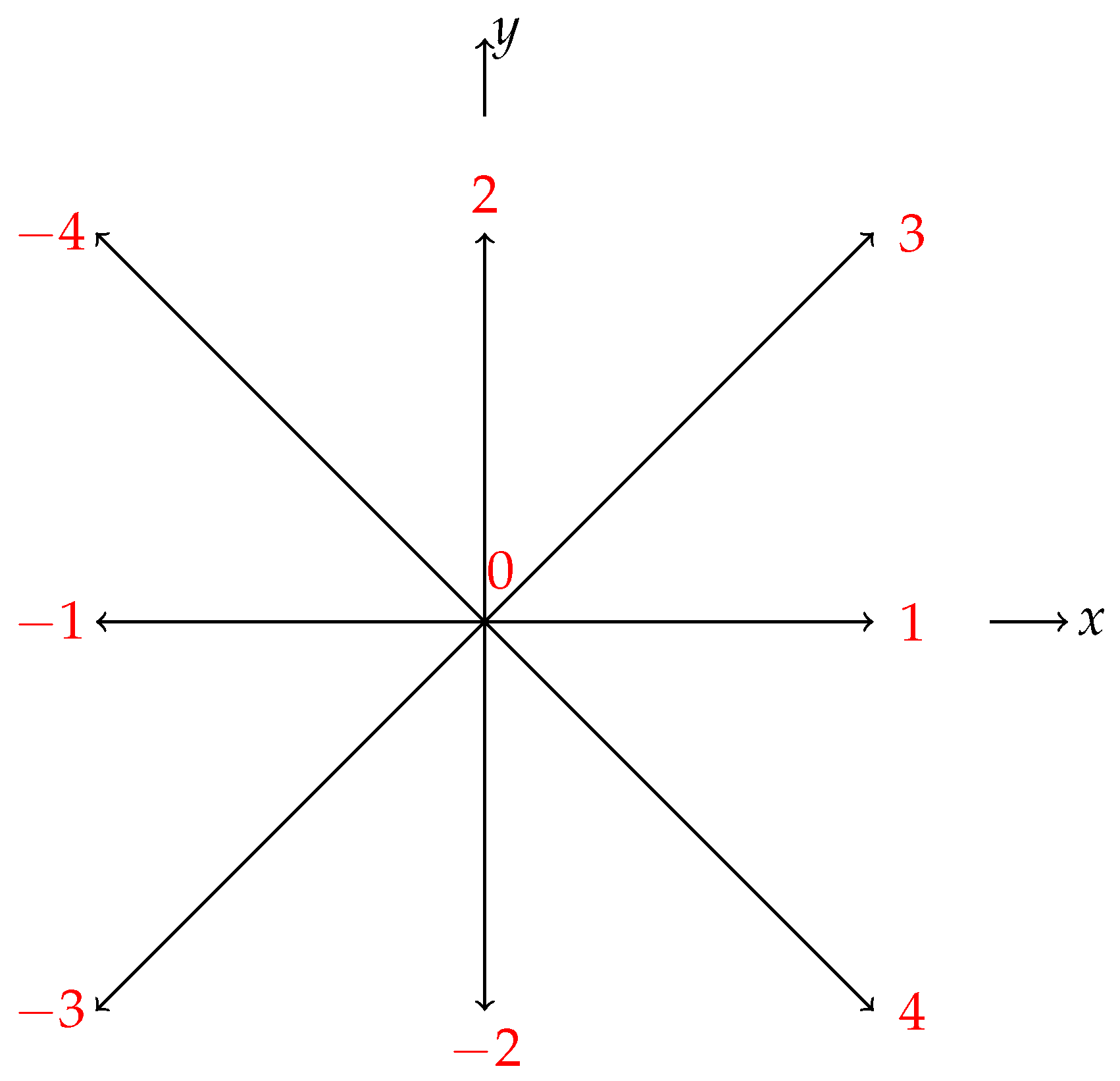
5. Nine Velocity DV Boltzmann Model for $\mathit{D}\mathbf{2}\mathit{Q}\mathbf{9}$ Lattice

We consider the DV Boltzmann model on a nine-velocity lattice (Figure 1). This lattice is popular in LB theory [3], since the corresponding LB model recovers hydrodynamics at small Mach numbers limit and, in addition, its numerical implementation is very simple. For this model, we have three types of discrete velocities: zero velocity ${\mathit{c}}_0=(0,0)$ with the weight $w_0=16/36$; four velocities, parallel to $x,y$ axes, i.e., ${\mathit{c}}_{\pm 1}=(\pm 1,0)c,{\mathit{c}}_{\pm 2}=(0,\pm 1)c$ with the weight $w_0=4/36$; four diagonal velocities ${\mathit{c}}_{\pm 3}=(\pm 1,\pm 1)c,{\mathit{c}}_{\pm 4}=(\pm 1,\mp 1)c$ with the weight $w_0=1/36$—here, c is the positive constant. The lattice velocity magnitudes for these three groups are $0,c,\sqrt{2}c$. Moreover, ${\theta }_0={\sum }_i{w}_i{c}_i^2=c^2/3$.

It is well-known that these lattice velocities and weights satisfy the conditions (3), (20) and (21); therefore, if it is possible to construct the collisions in such a way that the mass and momentum are conserved then the Euler equations are satisfied. We mention that the lattices and collision rules for DV Boltzmann models, which can potentially recover the hydrodynamics, have been considered previously [46,47]—for instance, the model with single-relaxation time describing Navier–Stokes equations has been proposed [46,47]. In here we consider only the collisions for the nine-bit lattice in a more detailed way; the considered model is of the multiple-relaxation-time type:

a.

Broadwell type collision is the reaction between the particles 1 and $-1$, which turn into the particles 2 and $-2$ (Figure 1); schematically, we can denote this reaction as $(1,-1)⟶(2,-2)$. The contribution of this collision to right side of (1) denoted as $J_0$ is as follows

$$J_0=f_{-2}{f}_2-f_{-1}{f}_1;$$

(25)

b.

the collisions linking all three different energy states, they define transitions between the particle’s states with different kinetic energies, and evidently can not be excluded. We have four different reactions $(1,2)⟶(0,3)$, $(1,-2)⟶(0,4)$, $(-1,-2)⟶(0,-3)$, $(-1,2)⟶(0,-4)$. The corresponding contributions to the collision kernel are

$$\begin{array}{cc}\hfill & J_1=f_0{f}_3-f_1{f}_2,J_2=f_0{f}_4-f_1{f}_{-2},\hfill \\ \hfill & J_3=f_0{f}_{-4}-f_{-1}{f}_2,J_4=f_0{f}_{-3}-f_{-1}{f}_{-2};\hfill \end{array}$$

(26)

c.

Broadwell type collision between the particles with the velocity magnitudes $\sqrt{2}c$ is defined by the reaction $(3,-3)⟶(4,-4)$, the contributions to the collision kernel are

$$J_5=f_{-4}{f}_4-f_{-3}{f}_3;$$

(27)

d.

the collisions between the particles with the velocity magnitudes $\sqrt{2}c$ and c, we have four different reactions $(-4,1)⟶(-1,3),(-3,1)⟶(-1,4),(-3,2)⟶(-4,-2),(4,2)⟶(-2,3)$, the contributions to the collision kernel are

$$\begin{array}{cc}\hfill & J_6=f_3{f}_{-1}-f_{-4}{f}_1,J_7=f_{-1}{f}_4-f_{-3}{f}_1,\hfill \\ \hfill & J_8=f_{-4}{f}_{-2}-f_{-3}{f}_2,J_9=f_3{f}_{-2}-f_4{f}_2.\hfill \end{array}$$

(28)

The collisions (25)–(28) conserve mass, momentum and energy; the corresponding $D2Q9$ DV Boltzmann model reads as

$$\begin{array}{cc}\hfill & \frac{\partial f_1}{\partial t}+c\frac{\partial f_1}{\partial x}=\alpha J_0+\beta (J_1+J_2)+\lambda (J_6+J_7),\hfill \end{array}$$

(29)

$$\begin{array}{cc}\hfill & \frac{\partial f_{-1}}{\partial t}-c\frac{\partial f_{-1}}{\partial x}=\alpha J_0+\beta (J_3+J_4)-\lambda (J_6+J_7),\hfill \end{array}$$

(30)

$$\begin{array}{cc}\hfill & \frac{\partial f_2}{\partial t}+c\frac{\partial f_2}{\partial y}=-\alpha J_0+\beta (J_1+J_3)+\lambda (J_8+J_9),\hfill \end{array}$$

(31)

$$\begin{array}{cc}\hfill & \frac{\partial f_{-2}}{\partial t}-c\frac{\partial f_{-2}}{\partial y}=-\alpha J_0+\beta (J_2+J_4)-\lambda (J_8+J_9),\hfill \end{array}$$

(32)

$$\begin{array}{cc}\hfill & \frac{\partial f_3}{\partial t}+c\frac{\partial f_3}{\partial x}+c\frac{\partial f_3}{\partial y}=\gamma J_5-\beta J_1-\lambda (J_6+J_9),\hfill \end{array}$$

(33)

$$\begin{array}{cc}\hfill & \frac{\partial f_{-3}}{\partial t}-c\frac{\partial f_{-3}}{\partial x}-c\frac{\partial f_{-3}}{\partial y}=\gamma J_5-\beta J_4+\lambda (J_7+J_8),\hfill \end{array}$$

(34)

$$\begin{array}{cc}\hfill & \frac{\partial f_4}{\partial t}+c\frac{\partial f_4}{\partial x}-c\frac{\partial f_4}{\partial y}=-\gamma J_5-\beta J_2+\lambda (-J_7+J_9),\hfill \end{array}$$

(35)

$$\begin{array}{cc}\hfill & \frac{\partial f_{-4}}{\partial t}-c\frac{\partial f_{-4}}{\partial x}+c\frac{\partial f_{-4}}{\partial y}=-\gamma J_5-\beta J_3+\lambda (J_6-J_8),\hfill \end{array}$$

(36)

$$\begin{array}{cc}\hfill & \frac{\partial f_0}{\partial t}=-\beta (J_1+J_2+J_3+J_4),\hfill \end{array}$$

(37)

where $\alpha ,\beta ,\lambda ,\gamma$ in (29)–(37) are positive transition probabilities. Now, we can consider the analogs of the Navier–Stokes equations for the model (29)–(37).

Proposition 3.

The Equations (29)–(37) lead to Navier–Stokes equations for nearly incompressible flows with errors of order $O\left({\Delta }^3\right)$ if

$$4\alpha =\gamma +4\beta +4\lambda ,$$

(38)

the shear viscosity ν equals

$$\nu =\frac{3}{4\alpha }.$$

(39)

Proof. 

From (22), one can deduce that the corrections to the DV distribution function $f_i^{\left(1\right)}$ corresponding to the viscous terms can be represented as a linear combination of $\frac{d{f}_i^{eq}}{dt}$ terms. In the case of nearly incompressible flow, these terms can be represented as (Formula $\left(2.12\right)$ in [2])

$$\frac{d{f}_i^{eq}}{dt}=w_i\frac{{\mathit{c}}_{\mathit{i}}{\mathit{c}}_{\mathit{i}}}{{\theta }_0}:\frac{\partial }{\partial r}\Delta \mathit{u},$$

(40)

where $\frac{\partial }{\partial r}=(\frac{\partial }{\partial x},\frac{\partial }{\partial y})$. According (23) we can try add the terms proportional $div(\Delta \mathit{u})$, but they equal zero for the incompressible limit; then, we seek the solution in the form

$$f_i^{\left(1\right)}=a_i{\mathit{Q}}_{\mathit{i}},{\mathit{Q}}_{\mathit{i}}=w_i\frac{{\mathit{c}}_{\mathit{i}}{\mathit{c}}_{\mathit{i}}}{{\theta }_0}:\frac{\partial }{\partial r}\Delta \mathit{u},$$

(41)

where the coefficients $a_i$ are equal for the indexes i corresponding to the discrete velocities ${\mathit{c}}_{\mathit{i}}$ with the same kinetic energy. The substitution of (41) into (29)–(37) leads to three algebraic equations for the coefficients $a_i$, (29)–(32) yield the first equation

$$3w_1\frac{\partial }{\partial x}\Delta u_x=2\alpha w_1{a}_1(\frac{\partial }{\partial y}\Delta u_y-\frac{\partial }{\partial x}\Delta u_x)=$$

$$=2\alpha w_1{a}_1(\frac{\partial }{\partial y}\Delta u_y-\frac{\partial }{\partial x}\Delta u_x-div(\Delta \mathit{u}))=-4\alpha w_1{a}_1\frac{\partial }{\partial x}\Delta u_x,$$

from which we obtain

$$a_1=-\frac{3}{4\alpha },$$

(33)–(36) yield the second equation

$$3w_2(\frac{\partial }{\partial x}\Delta u_y+\frac{\partial }{\partial y}\Delta u_x)=-(4\gamma w_2+\beta w_0+4\lambda w_1)a_2(\frac{\partial }{\partial x}\Delta u_y+\frac{\partial }{\partial y}\Delta u_x),$$

then

$$a_2=-\frac{3w_2}{4\gamma w_2+\beta w_0+4\lambda w_1}.$$

The third equation, which can be obtained from (37) is satisfied automatically. Now, with the exact expressions for $a_1,a_2$, we can evaluate $f_i^{\left(1\right)}$ and the viscous corrections to the pressure tensor ${\mathit{P}}^{\left(1\right)}={\sum }_i{f}_i^{\left(1\right)}{\mathit{c}}_{\mathit{i}}{\mathit{c}}_{\mathit{i}}$. Then, the Navier–Stokes viscous terms can be evaluated as

$$-\sum _{\sigma }\frac{\partial }{\partial r_{\sigma }}{P}_{\eta \sigma }^{\left(1\right)}=-\sum _{\sigma }\frac{\partial }{\partial r_{\sigma }}\left(\sum _i{f}_i^{\left(1\right)}{\mathit{c}}_{\mathit{i},\mathit{\eta }}{\mathit{c}}_{\mathit{i},\mathit{\sigma }}\right),$$

where $\sigma ,\eta$ equal x or y. For instance,

$$-\frac{\partial }{\partial x}{P}_{xx}^{\left(1\right)}-\frac{\partial }{\partial y}{P}_{xy}^{\left(1\right)}=\frac{3}{2\alpha }\frac{{\partial }^2}{\partial x^2}\Delta u_x+\frac{12w_2}{4\gamma w_2+\beta w_0+4\lambda w_1}(\frac{{\partial }^2}{\partial x\partial y}\Delta u_y+\frac{{\partial }^2}{\partial y^2}\Delta u_x)$$

we require $4\alpha =\gamma +4\beta +4\lambda$, then by applying $div(\Delta \mathit{u})=0$ we finally obtain

$$-\frac{\partial }{\partial x}{P}_{xx}^{\left(1\right)}-\frac{\partial }{\partial y}{P}_{xy}^{\left(1\right)}=\frac{3}{4\alpha }(\frac{{\partial }^2}{\partial x^2}+\frac{{\partial }^2}{\partial y^2})\Delta u_x,$$

therefore $\nu =3/4\alpha$. □

For the model (29)–(37), there are ten collisions. If we consider all reaction vectors and the corresponding collision matrix, one can convince that $rank\left(C\right)=5$, the number of the discrete velocities $N=9$. This means that we do not have any collision invariants except mass, momentum, energy (Proposition 2). We can exclude up to five reactions from the model; for instance, we can keep only the Broadwell collisions (type a.) and the collisions of type b., i.e., we set $\gamma =\lambda =0$. On the other side, the numerical simulations show that the addition of the collisions from the group c. or d. enhances the stability properties.

Finally, we emphasize that, for the model (29)–(37), all the collisions conserve energy (elastic). Generally speaking, this is not necessary because we are focused on the correct reproduction of the mass and momentum equations. For instance, it is possible to construct the model of DV Boltzmann type in one spatial dimension with inelastic collisions [26] (quasi-chemical model with three discrete velocities) which leads to the correct Navier–Stokes equation at small Mach limit.

6. Numerical Implementation and Test Problems

The model is implemented similarly to the conventional LB $D2Q9$ model [3]. Firstly, we perform the collision step, then post-collision distribution functions are streamed at appropriate directions. It is well-known from the LB theory that the discretization of space–time affects the viscosity. The DV Boltzmann model discretized in a similar form as LB model reads as

$$f_i(t+\delta t,\mathit{r}+{\mathit{c}}_{\mathit{i}}\delta t)-f_i(t,\mathit{r})=I_i[f_1,\dots f_N](t,\mathit{r})\delta t,$$

(42)

by applying the Taylor expansion this equation can be rewritten as

$$(\frac{\partial }{\partial t}+{\mathit{c}}_{\mathit{i}}\frac{\partial }{\partial \mathit{r}})f_i(t,\mathit{r})\delta t+\frac{1}{2}{(\frac{\partial }{\partial t}+{\mathit{c}}_{\mathit{i}}\frac{\partial }{\partial \mathit{r}})}^2{f}_i(t,\mathit{r})\delta t^2+O\left(\delta t^3\right)=I_i[f_1,\dots f_N](t,\mathit{r})\delta t,$$

then

$$(\frac{\partial }{\partial t}+{\mathit{c}}_{\mathit{i}}\frac{\partial }{\partial \mathit{r}})f_i(t,\mathit{r})=I_i[f_1,\dots f_N](t,\mathit{r})-\frac{1}{2}{(\frac{\partial }{\partial t}+{\mathit{c}}_{\mathit{i}}\frac{\partial }{\partial \mathit{r}})}^2{f}_i(t,\mathit{r})\delta t+O\left(\delta t^2\right),$$

therefore, we can conclude that the scheme (42) led to the hydrodynamic equations in which the contributions from $-\frac{1}{2}{(\frac{\partial }{\partial t}+{\mathit{c}}_{\mathit{i}}\frac{\partial }{\partial \mathit{r}})}^2{f}_i(t,\mathit{r})\delta t+O\left(\delta t^2\right)=-\frac{\delta t}{2}\frac{d^2}{d{t}^2}{f}_i+O\left(\delta t^2\right)$ are present. The additional terms for the Navier–Stokes equations can be obtained with the application of the Chapman–Enskog expansion [3]. Note that the terms $O\left(\delta t^2\right)$ do not affect the Navier–Stokes equations, since they contain third order derivatives, which, in the Chapman–Enskog multiple-scale expansion, enter the equations for the moments at the Burnett level. For the Navier–Stokes equation, the additional viscosity terms result from $-\frac{\delta t}{2}\frac{d^2}{d{t}^2}{f}_i^{eq}$, its contribution to $\frac{\partial }{\partial \mathit{r}}·{\mathit{P}}^{\left(1\right)}$ is $\frac{\delta t}{2}{\sum }_i{\mathit{c}}_{\mathit{i}}{\mathit{c}}_{\mathit{i}}·\frac{d}{d\mathit{r}}\frac{d}{dt}{f}_i^{eq}$, remembering that $\frac{d}{dt}{f}_i^{eq}$ can be expressed by (40), we eventually obtain $\frac{\delta t}{6}(\frac{{\partial }^2}{\partial x^2}+\frac{{\partial }^2}{\partial y^2})\mathit{u}$.

Then, for the DV $D2Q9$ Boltzmann model in the form (42), the viscosity is given by

$$\nu =\frac{3}{4\alpha }-\frac{\delta t}{6}.$$

In the simulations, the parameters are taken as follows

$$\alpha =\frac{3}{4(\nu +\frac{\delta t}{6})},\beta =0.25\alpha ,\gamma =4\alpha -4\beta =3\alpha ,\lambda =0,$$

(43)

i.e., we have six different collisions.

To validate the second-order convergence of the presented scheme, we estimate the simulation error defined as

$$error=\frac{\sqrt{{\sum }_z{(u_m\left(z\right)-u_{bench}\left(z\right))}^2}}{\sqrt{{\sum }_z{u}_{bench}{\left(z\right)}^2}},$$

(44)

where z denotes the spatial variable, $u_m,u_{bench}$ are the modeled variable (velocity) and the benchmark solution, respectively. The convergence rate is evaluated by fitting the values of $log\left(error\right)$ for the various $log\left(h\right)=log\left(\frac{1}{N}\right)$ (N is the number of the lattice nodes, h is proportional to the lattice spacing) using the linear regression, the second-order convergence is achieved if the regression slope coefficient is close to 2.

Compared to LB $D2Q9$ model, the scheme (29)–(37) differs only in the collision term and the expression for the viscosity. This means that the computation time for (29)–(37) implemented in the form (42) is approximately the same as for LB $D2Q9$ model.

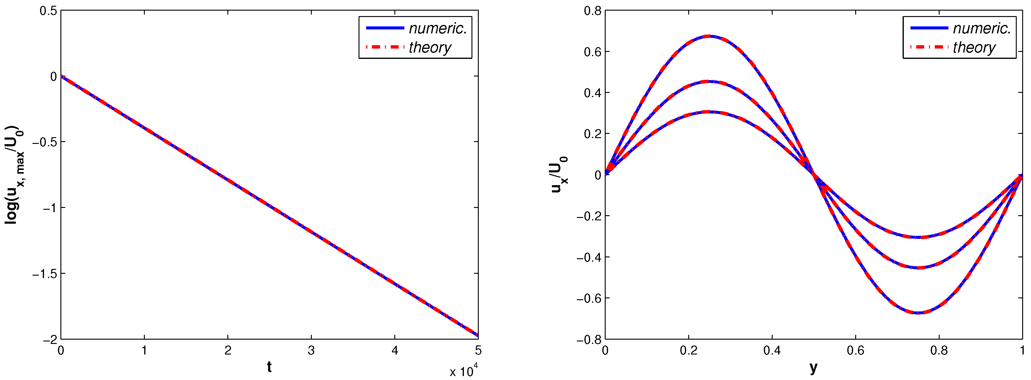
6.1. Shear Wave Decay

We consider the dynamics in terms of the time of the sinusoidal velocity wave in a square domain. The initial flow velocity in x direction is dependent on y coordinate and is given by

$$u_x(x,y,t=0)=U_{0}sin\left(ky\right),k=\frac{2\pi }{L},$$

where L is the length of the domain equals N lattice nodes and $U_0=0.01$. The periodic boundary conditions are applied for the present problem. This problem has the following analytical solution

$$u_x(x,y,t)=U_{0}sin\left(ky\right)e^{-\nu k^{2}t}.$$

In the present case, we consider $\nu =0.001$ and $N=101$, the time step $\delta t=1$. We compare the analytical solutions with the velocity profiles obtained by the application of the model (29)–(37) (implemented in the form (42)). The peak velocity time history and the velocity profiles for the different moments of time are plotted, Figure 2. One can see that the simulation results are very similar to the analytical profiles.

It is worth mentioning that it is possible to shorten the model and take $\gamma =\lambda =0$, in this case $\alpha =\beta$, and we have only five different collisions. The numerical experiments show that this model becomes unstable for $\nu <0.1$, while the setting (43) allows to model the flow with small viscosity and no instabilities are observed.

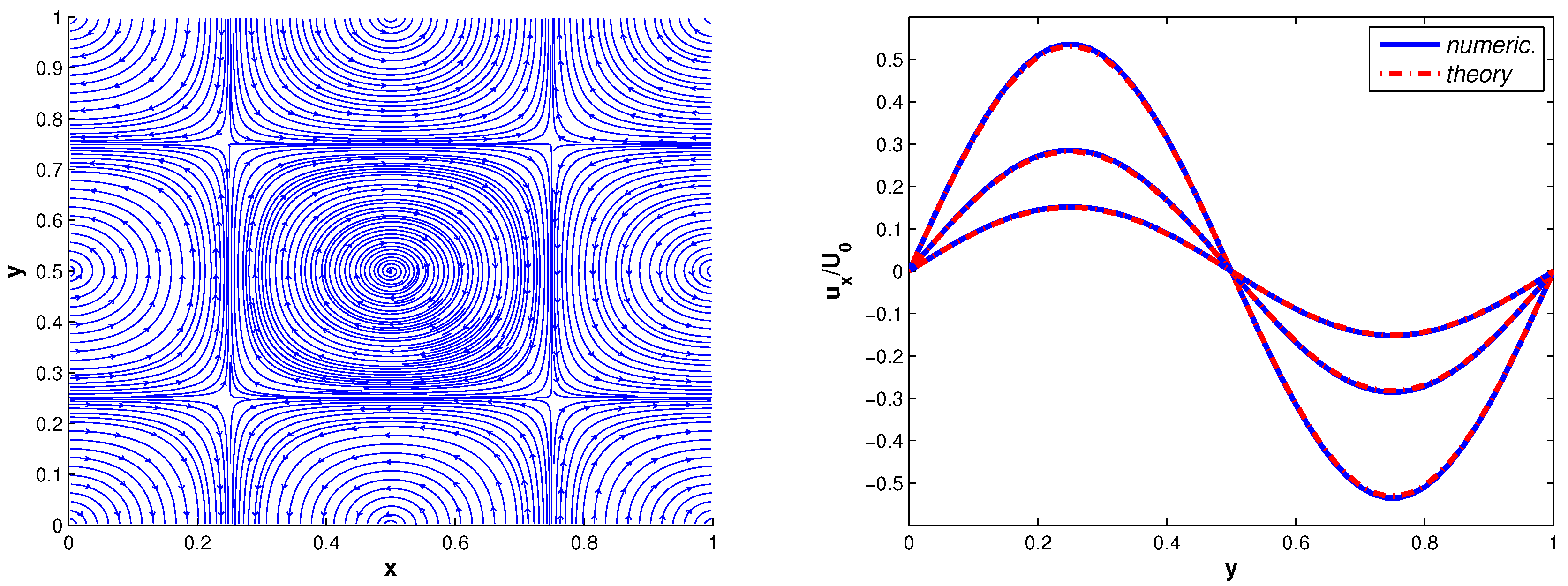
6.2. Taylor-Green Vortex

Similarly to the previous problem, we consider a square domain, and the initial velocity field is given by the formula

$$u_x(x,y,t=0)=-U_{0}cos\left(kx\right)sin\left(ky\right),u_y(x,y,t=0)=U_{0}sin\left(kx\right)cos\left(ky\right),$$

where the size of the domain is $L\times L$ (or $N\times N$ in lattice units, where N is the number of the lattice nodes) and $k=\frac{2\pi }{L}$. The periodic boundary conditions are applied. For the present problem we set $U_0=0.01,\nu =0.001,N=51$, the time step $\delta t=1$. The analytical solution to the problem is as follows

$$u_x(x,y,t)=-U_{0}cos\left(kx\right)sin\left(ky\right)e^{-2\nu k^{2}t},u_y(x,y,t)=U_{0}sin\left(kx\right)cos\left(ky\right)e^{-2\nu k^{2}t},$$

one can see that the initial structure of the velocity field persists in time, and only uniform decay of the velocity amplitudes is observed. The numerical simulations for the model (29)–(37) (implemented in the form (42)) show that the form of the velocity field does not change. We also present the behavior of the velocity $u_x(x,y=L/2,t)$ over time, obtained analytically and numerically for three different moments of time; obviously, both approaches give very similar profiles (Figure 3).

Finally, we consider the convergence rates of the numerical simulation results to the benchmark solutions. This can be performed by considering the logarithms of the simulation errors (44) for the different values of $log\left(h\right)=log(1/N)$. In the present case, we take $N=25,49,73,101$. In Figure 4, the logarithms of the errors of the velocities are presented for DV and the conventional LB $D2Q9$ models; the results are very similar for both models. One can see that the estimated slope values are close to 2; this indicates that the proposed scheme is accurate in the second-order.

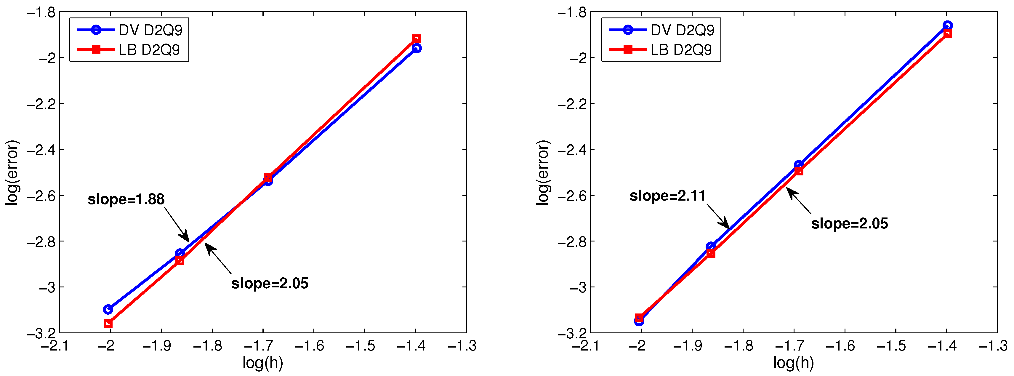
7. Results and Discussion

In this paper, we have considered the DV Boltzmann model applicable to the modeling of viscous quasi-incompressible flows at a small Mach number limit. The presented model has the same discrete velocity structure and absolute equilibrium as LB $D2Q9$, but the collision rules for the particles are postulated exactly. There are four types of collision and ten possible different collisions; the unique transition probability corresponds to all possible reactions in the group. Moreover, these collisions conserve only mass, momentum and energy (spurious invariants do not exist). In terms of LB theory, this model can be considered as a scheme with multiple relaxation times. Note that the H-theorem is valid for the model by construction (at least for the continuous space–time variables).

We have demonstrated that DV Boltzmann equations can be a viable tool in modeling of hydrodynamic flows. The shear wave decay and Taylor–Green vortex have been considered as benchmark problems. The comparison of the simulation results with the analytical solutions has shown good accuracy.

One of the most intriguing problems is the evaluation of the stability properties of the presented DV Boltzmann system and the optimal choice of transition probabilities. One can expect that the DV Boltzmann model for $D2Q9$ lattice has a better stability than the conventional LB $D2Q9$ model, since the H-theorem is satisfied. In order to elucidate this issue, one can consider additional problems like Sod shock tube, double shear layer and lid-driven cavity. These problems are left for future study.

References

1. Kogan, M. Rarefied Gas Dynamics; Plenum Press: New York, NY, USA, 1969. [Google Scholar]
2. Guo, Z.; Shu, C. Lattice Boltzmann Method and Its Applications in Engineering; World Scientific Publishing Company: Singapore, 2013. [Google Scholar]
3. Krüger, T.; Kusumaatmaja, H.; Kuzmin, A.; Shardt, O.; Silva, G.; Viggen, E. The Lattice Boltzmann Method. Principles and Practice; Springer: Berlin/Heidelberg, Germany, 2017. [Google Scholar]
4. Succi, S. The Lattice Boltzmann Equation: For Complex States of Flowing Matter; OUP: Oxford, UK, 2018. [Google Scholar]
5. Lallemand, P.; Luo, L.S.; Krafczyk, M.; Yong, W.A. The lattice Boltzmann method for nearly incompressible flows. J. Comput. Phys. 2020, 431, 109713. [Google Scholar] [CrossRef]
6. Qian, Y.H.; d’Humières, D.; Lallemand, P. Lattice BGK models for Navier-Stokes equation. Europhys. Lett. 1992, 17, 479–484. [Google Scholar] [CrossRef]
7. Toschi, F.; Succi, S. Lattice Boltzmann method at finite Knudsen numbers. Europhys. Lett. 2005, 69, 549. [Google Scholar] [CrossRef] [Green Version]
8. Ansumali, S.; Karlin, I. Consistent Lattice Boltzmann Method. Phys. Rev. Lett. 2005, 95, 260605. [Google Scholar] [CrossRef] [Green Version]
9. Shan, X.; Yuan, X.; Chen, H. Kinetic theory representation of hydrodynamics: A way beyond the Navier–Stokes equation. J. Fluid Mech. 2006, 550, 413–441. [Google Scholar] [CrossRef]
10. Zhang, R.; Shan, X.; Chen, H. Efficient kinetic method for fluid simulation beyond the Navier-Stokes equation. Phys. Rev. E 2006, 74, 046703. [Google Scholar] [CrossRef] [Green Version]
11. Ansumali, S.; Karlin, I.; Arcidiacono, S.; Abbas, A.; Prasianakis, N. Hydrodynamics beyond Navier-Stokes: Exact Solution to the Lattice Boltzmann Hierarchy. Phys. Rev. Lett. 2007, 98, 124502. [Google Scholar] [CrossRef] [Green Version]
12. Niu, X.; Hyodo, S.; Munekata, T.; Suga, K. Kinetic lattice Boltzmann method for microscale gas flows: Issues on boundary condition, relaxation time, and regularization. Phys. Rev. E 2007, 76, 036711. [Google Scholar] [CrossRef]
13. Kim, S.; Pitsch, H.; Boyd, I. Accuracy of higher-order lattice Boltzmann methods for microscale flows with finite Knudsen numbers. J. Comput. Phys. 2008, 227, 8655. [Google Scholar] [CrossRef]
14. Tang, G.; Zhang, Y.; Emerson, D. Lattice Boltzmann models for nonequilibrium gas flows. Phys. Rev. E 2008, 77, 046701. [Google Scholar] [CrossRef] [Green Version]
15. Meng, J.; Zhang, Y. Gauss-Hermite quadratures and accuracy of lattice Boltzmann models for non-equilibrium gas flows. Phys. Rev. E 2011, 83, 036704. [Google Scholar] [CrossRef] [Green Version]
16. Suga, K. Lattice Boltzmann methods for complex micro-flows: Applicability and limitations for practical applications. Fluid Dyn. Res. 2013, 45, 034501. [Google Scholar] [CrossRef]
17. Feuchter, C.; Schleifenbaum, W. High-order lattice Boltzmann models for wall-bounded flows at finite Knudsen numbers. Phys. Rev. E 2016, 94, 013304. [Google Scholar] [CrossRef] [Green Version]
18. Ambruş, V.; Sofonea, V. Lattice Boltzmann models based on half-range Gauss–Hermite quadratures. J. Comp. Phys. 2016, 316, 760–788. [Google Scholar] [CrossRef]
19. Ilyin, O. Gaussian Lattice Boltzmann method and its applications to rarefied flows. Phys. Fluids 2020, 32, 012007. [Google Scholar] [CrossRef]
20. Wagner, A. An H-theorem for the lattice Boltzmann approach to hydrodynamics. Europhys. Lett. 1998, 44, 144–149. [Google Scholar] [CrossRef] [Green Version]
21. Yong, W.A.; Luo, L.S. Nonexistence of H theorems for the athermal lattice Boltzmann models with polynomial equilibria. Phys. Rev. E 2003, 67, 051105. [Google Scholar] [CrossRef] [Green Version]
22. Yong, W.A.; Luo, L.S. Nonexistence of H Theorem for some Lattice Boltzmann models. J. Stat. Phys. 2005, 121, 91–103. [Google Scholar] [CrossRef] [Green Version]
23. Karlin, I.; Ferrante, A.; Öttinger, H. Perfect entropy functions of the Lattice Boltzmann method. Europhys. Lett. 1999, 47, 182–188. [Google Scholar] [CrossRef] [Green Version]
24. Ansumali, S.; Karlin, I.; Öttinger, H. Minimal entropic kinetic models for hydrodynamics. Europhys. Lett. 2003, 63, 798–804. [Google Scholar] [CrossRef] [Green Version]
25. Karlin, I.; Ansumali, S.; Frouzakis, C.; Chikatamarla, S. Elements of the Lattice Boltzmann Method I: Linear Advection Equation. Commun. Comput. Phys. 2006, 1, 616–655. [Google Scholar]
26. Karlin, I.; Chikatamarla, S.; Ansumali, S. Elements of the lattice Boltzmann method II: Kinetics and hydrodynamics in one dimension. Commun. Comput. Phys. 2007, 2, 196–238. [Google Scholar]
27. Broadwell, J. Shock structure in a simple discrete velocity gas. Phys. Fluids 1964, 7, 1243–1247. [Google Scholar] [CrossRef]
28. Godunov, S.; Sultangazin, U. On discrete models of the kinetic Boltzmann equation. Russ. Math. Surv. 1971, 26, 1–56. [Google Scholar] [CrossRef]
29. Gatignol, R. The hydrodynamical description for a discrete velocity model of gas. Complex Syst. 1987, 1, 709–725. [Google Scholar]
30. Platkowski, T.; Illner, R. Discrete velocity models of the Boltzmann equation: A survey on the mathematical aspects of the theory. SIAM Rev. 1988, 30, 213–255. [Google Scholar] [CrossRef]
31. Bobylev, A.; Spiga, G. On a class of exact two-dimensional stationary solutions for the Broadwell model of the Boltzmann equation. J. Phys. A Math. Gen. 1994, 27, 7451–7459. [Google Scholar] [CrossRef]
32. Bobylev, A. Exact solutions of discrete kinetic models and stationary problems for the plane Broadwell model. Math. Methods Appl. Sci. 1996, 19, 825–845. [Google Scholar] [CrossRef] [Green Version]
33. Bobylev, A.; Toscani, G. Two dimensional half-space problems for the Broadwell discrete velocity model. Contin. Mech. Termodyn. 1996, 8, 257–274. [Google Scholar] [CrossRef]
34. Bobylev, A.; Caraffini, G.; Spiga, G. Non-stationary two-dimensional potential flows by the Broadwell model equations. Eur. J. Mech. B Fluids 2000, 19, 303–315. [Google Scholar] [CrossRef]
35. Ilyin, O. The analytical solutions of 2D stationary Broadwell kinetic model. J. Stat. Phys. 2012, 146, 67–72. [Google Scholar] [CrossRef]
36. Ilyin, O. Symmetries, the current function, and exact solutions for Broadwell’s two-dimensional stationary kinetic model. Theor. Math. Phys. 2014, 179, 679–688. [Google Scholar] [CrossRef]
37. Chen, H.; Goldhirsch, I.; Orszag, S. Discrete rotational symmetry, moment isotropy, and higher order lattice Boltzmann models. J. Sci. Comput. 2008, 34, 87–112. [Google Scholar] [CrossRef]
38. Uchiyama, K. On the Boltzmann-Grad limit for the Broadwell model of the Boltzmann equation. J. Stat. Phys. 1988, 52, 331–355. [Google Scholar] [CrossRef]
39. Bobylev, A.; Cercignani, C. Discrete velocity models without nonphysical invariants. J. Stat. Phys. 1999, 97, 677–686. [Google Scholar] [CrossRef]
40. Bobylev, A.; Vinerean, M. Construction of discrete kinetic models with given invariants. J. Stat. Phys. 2008, 132, 153–170. [Google Scholar] [CrossRef]
41. Vinerean, M.; Windfäll, Å.; Bobylev, A. Construction of normal discrete velocity models of the Boltzmann equation. Nuovo Cim. 2010, 33, 257–264. [Google Scholar]
42. Bernhoff, N.; Vinerean, M. Discrete velocity models for mixtures without nonphysical collision invariants. J. Stat. Phys. 2016, 165, 434–453. [Google Scholar] [CrossRef] [Green Version]
43. Chauvat, P.; Gatignol, R. Euler and Navier-Stokes description for a class of discrete models of gases with different moduli. Transp. Theory Stat. Phys. 1992, 21, 417–435. [Google Scholar] [CrossRef]
44. Vedenyapin, V.; Orlov, Y. Conservation laws for polynomial Hamiltonians and for discrete models of the Boltzmann equation. Theor. Math. Phys. 1999, 121, 1516–1523. [Google Scholar] [CrossRef]
45. Vedenyapin, V. Velocity inductive construction for mixtures. Transp. Theor. Stat. Phys. 1999, 28, 727–742. [Google Scholar] [CrossRef]
46. Babovsky, H. “Small” kinetic models for transitional flow simulations. AIP Conf. Proc. 2012, 1501, 272–278. [Google Scholar]
47. Babovsky, H. Discrete kinetic models in the fluid dynamic limit. Comput. Math. with Appl. 2014, 67, 256–271. [Google Scholar] [CrossRef]
Figure 1. Two-dimensional nine-velocity lattice ( D 2 Q 9 ). Lattice velocities are labeled by red color.
Mathematics 09 00993 g001
Figure 2. Shear wave decay. The logarithm of the peak velocity time histories obtained numerically and analytically are presented (first slide); velocity profiles at different moments of time ( t = 10 5 , t = 2 × 10 5 , t = 3 × 10 5 ) obtained numerically and analytically are presented (second slide), the spatial variable y is normalized on the domain length L.
Mathematics 09 00993 g002
Figure 3. Taylor–Green vortex. The velocity streamlines are presented in the (first slide). The velocity profiles u x ( x , y = L / 2 , t ) for three different moments of time t = 2 × 10 4 , t = 4 × 10 4 , t = 6 × 10 4 obtained analytically and numerically are presented (second slide), and the spatial variables x , y are normalized on the domain length L.
Mathematics 09 00993 g003
Figure 4. Convergence rates for the shear wave decay and Taylor–Green vortex problems are shown. The results are obtained by applying DV and the conventional LB D 2 Q 9 models. In the (first slide) (shear wave decay), the logarithms of the errors (44) for the velocity u x ( y , t ) computed at the moment of time t = 1 / ( ν k 2 ) are presented; in the (second slide) (Taylor–Green vortex), the logarithms of the errors of the velocity u x ( x , y = L / 2 , t ) computed at the moment of time t = 1 / ( 2 ν k 2 ) are presented, where the variable h is proportional to the lattice spacing. The slope estimates are obtained by fitting the values of log ( e r r o r ) using the linear regression.
Mathematics 09 00993 g004
Publisher’s Note: MDPI stays neutral with regard to jurisdictional claims in published maps and institutional affiliations.